Chapter 15
Fraud Risk Assessments of Forensic Units
Monitoring means “to watch, and keep track of, or to check for some special purpose.” Continuous monitoring happens in many aspects of our personal life. Our water supply is continuously monitored, and all sorts of phenomena are monitored in commercial airplane flights. In hospitals, the monitoring of a patient's vital signs is taken for granted. In prisons, monitoring the activities and whereabouts of inmates is vital, and any escape is usually attributed to a lapse in monitoring activities. An Internet search for “continuous monitoring” will return results from applications such as monitoring storms, emissions, volcanoes, glucose for diabetics, perimeter activities for important installations, and foreign broadcasts for intelligence purposes. Since monitoring is so pervasive in everyday life it is puzzling that corporate transactions are not also the subject of continued monitoring to assess the risk of frauds or errors.
The 2006 edition of PricewaterhouseCoopers' (PWC) State of the Internal Audit Profession series reports that 81 percent of audit managers either had a continuous auditing or monitoring process in place, or that they were planning to develop one (PWC, 2006). Only one-half of audit managers had some actual form of continuous monitoring in place (possibly only one application). This low percentage might be due to a lack of guidance on methods and techniques that might be used in continuous monitoring applications. Of those that had a continuous monitoring application in place, 20 percent of these had fraud detection as the focus, and 10 percent focused their continuous monitoring activities on key performance indicators to identify deteriorating business activities. PWC (2006, 10) conclude that continuous auditing is still considered an emerging phenomenon, and is viewed by internal audit as a means to enhance their audit processes and to meet the stakeholder needs and demands for faster and higher-quality real-time assurance. PWC (2007a) paints a similar picture with 43 percent of respondents reporting the use of some form of continuous monitoring, but only 11 percent of respondents describing the process as fully operational. In 2006 and 2007 nearly one-fifth of audit managers did not have any form of continuous monitoring in place, nor did they have any plans to develop one. A lack of guidance on methods and techniques might be contributing to the low level of continuous monitoring. It is also possible that internal auditors expect the process owners to have a monitoring system in place.
PWC (2007b) predicts that over the next five years internal auditors will devote more time to risk management, fraud, internal controls, and process flows. Also, to remain relevant, auditors will need to adopt a comprehensive approach to audit and risk management, and will need to optimize the use of technology and conduct audits on a more targeted basis in response to specific risk concerns.
This chapter describes a system developed at a fast-food franchising company to monitor sales reports for errors, frauds, or omissions. The chapter describes the monitoring approach and includes some references to decision theory, fraud theory, and the deception cues literature. A case study is then described with a detailed description of the risk scoring method. Selected results and future plans for the system are then reviewed. The methodology could be adapted to other continuous monitoring and fraud risk assessment applications. The risk-scoring approach is developed further in the next chapter.
The risk score method was developed as a continuous monitoring system based on an adaptation of the IT-Monitoring framework of the International Federation of Accountants (IFAC, 2002). This adaptation gives the following steps in a continuous monitoring application:
- Determine the scope of the monitoring, and the methods and techniques to be applied
- Determine the indicators that will be used
- Design the system
- Document the system
- Record the findings
- Prepare management reports
- Update the system to improve the predictive ability of the system
One hurdle to getting started is that there are few, if any, documented methods and techniques. Without methods and techniques the rest of the steps in the framework cannot occur. Internal auditing standards state that in exercising due professional care the internal auditor should consider the use of computer-assisted audit tools and other data analysis techniques. The risk-scoring method is a computer-intensive forensic analytic technique.
The risk-scoring method uses a scoring system where the predictors are indicators of some attribute or behavior of interest. Examples of behaviors of interest include fraudulent baggage claims for an airline, check kiting by a bank customer, fraudulent vendors in a company, or fraudulent coupon claims against a manufacturer. The method applies to situations where the forensic investigator wants to score each forensic unit according to the risk of a specific type of fraud or error. A unit refers to one of the individuals or groups that together constitute a whole. A unit would also be one of a number of things that are equivalent or identical in function or form. A forensic unit is a unit that is being analyzed from a forensic perspective. Examples of forensic units could be:
- The frequent-flyer mileage account of an airline passenger
- A vendor submitting customer coupons to a manufacturer
- The sales reports of a franchisee
- The financial reports of operating divisions
- The income tax returns of individuals
- Bank accounts of bank customers
- An insurance adjuster at an insurance company
- A purchasing card of an employee
With the risk score method a risk score is calculated for each forensic unit. Higher scores reflect a higher risk of fraud or error. Forensic efforts can then be targeted at the highest scores.
The risk score method combines scores from several predictors. In the case study the behavior of interest was the underreporting of sales by fast-food franchise holders. A risk score of 0 is associated with a low risk of errors, and a risk score of 1 is associated with a high risk of errors. Each predictor is scored with a predictor risk score of 0 associated with a low risk of errors, and a predictor risk score of 1 is associated with a high risk of errors. Each predictor is weighted between 0 and 1 according to its perceived importance giving a final risk score based on the scores of the predictors and their weightings. This approach is similar to professors having various components in their classes (midterms, exams, quizzes, attendance, and assignments) with each component carrying a weight toward the final grade.
The predictors are chosen using professional judgment and industry knowledge. The goal is to try and capture mathematically what auditors are doing informally. The predictors are direct cues (clear signs of fraud) or indirect cues, which are similar to red flags. Red flag indicators are attributes that are present in a large percentage of fraud cases, although their presence in no way means that fraud is actually present in a particular case. For example, a vendor with the same address as an employee is a fact that is true in a large percentage of vendor fraud cases, but it does not mean that fraud is always present when a vendor has the same address as an employee. Risk-scoring applications usually target a very specific type of fraud.
Each predictor is scored so that each forensic unit ends up with a score from 0 to 1 for the predictor. The case study shows how the predictor values are converted to scores in the 0 to 1 range. The weights directly affect the final scores and because forensic units are ranked according to these scores, the weights affect the rankings and the fraud risk. The predictors can be seen to be the same as cues for decision making and the predictor weights to be the same as the weights given to the decision-making cues.
The weights used in decision making have been regularly discussed in psychological research studies. Slovic (1966) notes that little is known about the manner in which human subjects combine information from multiple cues, each with a probabilistic relationship to a criterion, into a unitary judgment about that criterion. A set of cues is consistent if the judge (decision maker) believed that the cues all agreed in their implications for the attributes being judged. Inconsistent cues would arise if the inferences that would be made from a subset of these cues would be contradicted by the implications of another set of cues. Consistency was seen to be a matter of degree and not an all-or-none matter. When a set of cues is consistent, each cue will be combined additively to reach a judgment. Inconsistent cues present a problem because the judge must either doubt the reliability of the cues or the belief in the correlation between the cues and the attributes being judged. In the risk-scoring methodology contradictory cues (predictors) would occur if one cue indicated a positive risk of fraud and another cue signaled “no fraud” with certainty. In the risk-scoring method, a score of 0 therefore means that the predictor seen alone suggests a low risk of fraud (and not a zero risk of fraud), and a score of 1 suggests a high risk of fraud (and not fraud with certainty). Because 0 and 1 mean low and high (and not zero risk, or certainty) we avoid contradictory cues.
The risk-scoring method also draws on the “theory of successful fraud detection” of Grazioli, Jamal, and Johnson (2006), which assumes that both the deceiver and the victim take into account the goals, knowledge, and possible actions of the other party. The deceiver cleverly manipulates the information cues. The detector also cleverly tries to reverse engineer the cues left by the deceiver and identifies them as symptoms of attempts to mislead. Detectors learn from experience to identify the deception tactics of the deceivers. These detection tactics are heuristics (trial and error methods) that evolve from (a) the discovery of an anomaly, (b) the belief that the anomaly is related to the goal of the deceiver, and (c), the belief that the anomaly could be the result of the deceiver's intentional manipulation. The risk-score method uses multiple predictors to assess the risk of fraud and also uses some reasonably sophisticated statistics including algebra, correlations, regressions, and mathematics related to Benford's Law.
The risk-score methodology combines scores from predictors into a final risk score from 0 to 1 with the scores closest to 1 indicating the highest risk of fraud. The predictors are based on various traits, which could be erratic numbers and deviations from expected patterns. A score of 0 indicates a low risk of fraud and a score of 1 indicates a high risk of fraud.
The Forensic Analytics Environment
The risk-score method was used in a company that operates about 5,000 franchised restaurants. The franchisees are required to report their monthly sales numbers within a few days after the end of the month. Based on the sales numbers reported by the franchisees, the franchisor bills the franchisee for royalty and advertising fees of approximately 7 percent of sales. The sales reports of the franchisees are processed by the accounts receivable department and time is needed to follow up on missing values and obvious errors. By the end of the second week of the month, the sales file for the preceding month is finalized. There is a continual reconciliation process that occurs to account for sales adjustments identified by the franchisees. By the 20th day of the month the sales numbers for the preceding month can usually be audited. This gives a short window before the sales reports for the next month come rolling in.
Sales-reporting errors (intentional or unintentional) are usually in the direction of understated sales and cause a revenue loss for the franchisor. Using the Vasarhelyi (1983) classification of errors, these errors could be (a) arithmetic errors, (b) integrity errors (unauthorized deletion of transactions), (c) timing errors (incorrect time period), (d) deliberate fraud, or (e) legal errors (transactions that violate legal clauses) such as omitting nonfood revenues. The cost of a revenue audit on location is high and the full cost is not only borne by the franchisor, but also partially by the franchisee in terms of the costs related to providing data, documents, and access to the electronics of the cash registers. The company needed a system of identifying high-risk sales reports. This environment is similar to many other situations where forensic units self-report dollar amounts and other statistics, and the recipient has to evaluate which of these might contain errors (e.g., financial statements submitted to the SEC, hazardous waste reports submitted to the EPA, airline baggage claims, and insurance claims).
The risk-scoring system was developed by the franchise audit section of internal audit. The work was done by two people and included developing an understanding of the players and the processes, the selection of the predictors, and computer programming (a combination of Excel and Access), data analysis, and first and subsequent proposals for scoring the predictors, and downloading franchisee data from the company's systems.
The team realized that it was not necessary to conduct an on-site audit for each restaurant thought to be high risk. Audits could either be done as field audits or correspondence audits, much like the approach taken by the IRS. Correspondence audits or desk audits could be conducted when the questions were limited in scope. Such audits are useful when only one or two areas of concern need to be addressed. Field audits are typically more thorough and are also intended to identify opportunities for operational improvements as well as the detection of sales underreporting.
The data used for the risk-scoring system was extracted from various financial and marketing systems. No potentially useful predictors were discarded because of a lack of data. The required data was downloaded to Excel files. The Excel data was imported into Access and all the analysis work and the reports were done in Access. An Access switchboard was used so that users could easily run and view the reports.
A Description of the Risk-Scoring System
Each franchised restaurant (called a location) was scored on 10 predictor variables. A score of 0 indicated a low risk of underreported sales, and a score of 1 indicated a high risk of underreported sales. The final result was a risk score between 0 and 1 based on a weighted average of the scores across the 10 predictors.
The original scoring objective for each predictor was to score one-third of the locations with 0, one-third of the locations with 1, and the remaining locations with evenly distributed scores from 0 to 1. This would give risk scores that were symmetrically distributed around the mean (something like the familiar bell-curve). The final scores would then also tend to be spread out as opposed to being clustered between (say) 0.40 and 0.44 where there is not much to distinguish the 50th highest score from the 500th highest score. The initial scoring objective was discarded in favor of a scoring system that more closely tracked low and high risks. The scoring objectives are shown graphically in Figure 15.1.
Figure 15.1 Initial Scoring Objective on the Left and the Achieved Scores on the Right
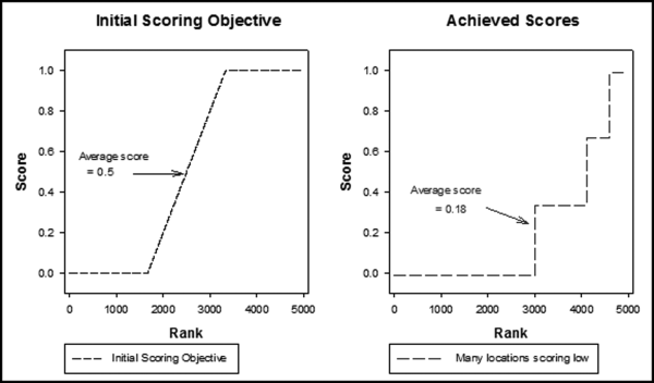
Figure 15.1 is a graphical depiction of the initial scoring objective and the final result for a typical predictor. The graphs in this chapter are a little more complex than usual and SigmaPlot 11 (www.sigmaplot.com) was used to prepare these graphics. It was not always possible to obtain a large (spread) variance for a single variable. For example, few locations actually used excessive round numbers and so relatively few locations would score 1.00 for that predictor.
Another scoring objective was to avoid the use of complex formulas (e.g., many nested “if” statements) because these are open to programming errors. In all cases where a formula included division (÷), care had to be taken to deal with the issues that arise when dividing by zero. Also, when a formula included taking either the log or square root of a number, care had to be taken to ensure that problems did not arise when trying to take the log or square root of a negative number. Division by zero or taking either the log or square root of a negative number gives an error message in Access and all subsequent uses of the calculated field have output errors.
The predictors and their weights were chosen based on the industry knowledge of the forensic investigators, their prior experiences, and to a small extent the available data. The system used 10 predictors and with hindsight, it seems that little would be added to the predictive value of the system if one or two more predictors were added. No predictors were considered as candidates for the risk scoring but then were later dropped because of a lack of data or other data issues such as data reliability. The predictors (abbreviated “P”) are discussed in the next sections.
P1: High Food and Supplies Costs
Franchisees are required to buy food and supplies (hereinafter “food”) from a selection of approved vendors. The food cost percentage is a key performance metric used by the company. A high food percentage is an indicator that (a) sales might be underreported, or (b) there is some significant shrinkage occurring at the franchisee level (possibly sales not being rung up by employees). This predictor is based on high values. A high values predictor is one where the values are high as compared to some norm. To determine what constitutes the norm, an analysis was needed of the food cost percentages across all locations. Figure 15.2 shows the analysis of food cost percentages to determine what is normal and what is excessive.
Figure 15.2 The Food Percentages and the Scores Applied to Those Percentages
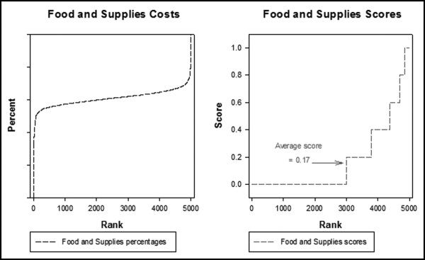
The analysis of the food cost percentages in Figure 15.2 shows a small set of locations with abnormally low scores and abnormally high scores (the extreme left and right sides of the graph in the left panel). The calculations of the past percentages includes cases where a franchisee that owns more than one location purchases from a vendor for location x1 and then later redistributes some of the food from location x1 to other locations. This fact, together with the fact that purchases in one month might not be used until the next month gives us the cases at the left and the right with abnormally low or high food cost percentages.
The past data showed that the average food cost as a proportion of sales across all locations was 0.305 and the standard deviation of these costs was 0.043. The median food cost proportion was 0.315. The table with the final P1 scoring formula is shown in Table 15.1.
Table 15.1 The Scoring Formula for the Food Cost Proportions.
| Food Proportion | Score | Notes |
| <= 0.31 | 0.0 | Average or slightly lower than average |
| 0.31 < Proportion <= 0.32 | 0.2 | Slightly higher than average |
| 0.32 < Proportion <= 0.33 | 0.4 | Higher than average |
| 0.33 < Proportion <= 0.34 | 0.6 | Much higher than average |
| 0.34 < Proportion <= 0.35 | 0.8 | High |
| Above 0.35 | 1.0 | Very high |
The graph of the P1 scores across all locations is shown in the right panel in Figure 15.2. About two-thirds of the locations scored a zero for P1 because they had food cost proportions that were close to average, or below average. The average score for P1 was just 0.17, because most restaurants had food costs near or below average.
P2: Very High Food and Supplies Costs
Even with the issues introduced by food transfers between locations and inventory changes from month-to-month, the food cost predictor was seen as being a reasonably reliable means of identifying underreported sales. Before the risk-scoring system, this was the only criteria used to select locations for audits. It was believed that P1 by itself did not do an adequate job of significantly raising the final scores of locations with high and very high food cost proportions. With P1 scored as is shown above, if the location did not also get high scores on the other nine predictors then a location with a food cost of 0.345 might end up with an average final risk score. P2 was added to give an extra boost to the scores of high and very high food cost locations. The P2 scoring formula is shown in Table 15.2.
Table 15.2 The Scoring Formula for the Second Predictor.
| Food Proportion | Score | Notes |
| <= 0.325 | 0.0 | Higher than average |
| 0.325 < Proportion <= 0.333 | 0.5 | Much higher than average |
| Above 0.333 | 1.0 | Very high |
The P2 predictor was used to raise the final scores of the restaurants thought to be high risk locations. The average score for P2 was 0.136, which shows that not too many locations scored 0.5 or 1.00 on this predictor. It is possible to combine the scores from P1 and P2 into a single predictor. Keeping them as two predictors makes it clearer to an investigator which locations are in the stratosphere when it comes to the food cost predictors.
The logic behind using a declining sales trend as a predictor was that as a franchisee underreported an ever increasing percentage of sales, its sales trend would be below average. This predictor can be classified as an opposite to expected predictor. These types of predictors work well because fraudsters often take their frauds to levels that would be obvious to anyone looking at the analytics. The Charlene Corley shipping costs example in the first chapter is an example of an extreme fraud. In an application based on frequent-flyer miles the forensic analytics identified passengers that had completed (say) a Miami to Los Angeles flight, and New York to London flight on the same day. In the franchising example, in a time of economic growth and some inflation the expectation is that sales will increase over time, even if the increase is quite mild. For example, true sales might be increasing by 6 percent per year, but reported sales might only increase by 1 percent per year. The first step was to calculate the overall sales trend and these results are shown in Figure 15.3.
Figure 15.3 The Changes in Annual Sales and the P3 Scores Applied to the Sales Percentage Changes
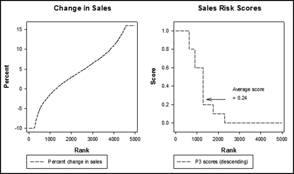
Figure 15.3 shows the sales changes for the past quarter against the same quarter one year earlier. The graph is truncated at −10 percent and +15 percent, which caused the two short straight lines on the left and right sides of the plotted line. About one-fifth of all locations had a sales decline and about four-fifths of the locations showed a year-on-year sales increase. All locations with sales changes that were below average were given a positive P3 score. The largest scores were for the largest quarter-on-quarter decreases. The P3 scoring formula is shown in Table 15.3.
Table 15.3 The Scoring Formula for the P3 Predictor Variable.
| Sales Change | Score | Notes |
| Less than −4 percent | 1.00 | Worst 15 percent of changes |
| −0.04 < Change <= −0.02 | 0.8 | Close to the largest declines |
| −0.02 < Change <= 0.00 | 0.6 | Slightly negative |
| 0.00 < Change <= 0.02 | 0.2 | Positive change, worse than average |
| 0.02 < Change <= 0.04 | 0.1 | Positive change, slightly worse than average |
| Above 4 percent | 0 | Better than average |
The scoring formula for P3 is a step formula in that a sales decrease of 2.2 percent and 3.7 percent are both scored as 0.80. In Access the formula is programmed using the SELECT function. Table 15.3 is easy for management and other users to understand. The formula above is open to some improvements using a little algebra so that −3.7 percent is given a higher score that −2.2 percent. The highest and the lowest scores are for changes less than −4.00 percent and higher than 4.00 percent. A possible function-based formula is shown in Equation 15.1 with  representing the change in Sales.
Using Equation (15.1), a sales change of −2.2 percent would be given a P3 score of 0.7750 and a sales change of −3.7 percent would be given a P3 score of 0.9625. The formula in Equation (15.1) is more precise but it might be difficult for management to understand how sales changes are related to P3 scores.
The goal for P4 was to score locations with an increasing food cost percentage as being high risk. The belief was that an upward shift in the food cost percentage over time is a sign of problems on the horizon or it could be an early stage fraud. This predictor is a high values predictor. The predictor uses the norm or average. In P4 high refers to a number being higher than the location's own historic averages.
For P4 the food cost proportion was based on the change over time. The monthly food cost percentages were quite variable because of food transfers and because large purchases in the final week of a month could distort the proportion for that month and for the following month. P4 was based on the slopes from linear regression equations run on several months of sales and food cost data.
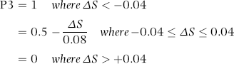
A comparison of the slopes indicated whether the food cost proportion was nudging upward. The sales numbers were on average about three times as large as the food cost numbers and consequently the sales slope was usually about three times as large as the food cost slope. The slopes of the sales numbers indicated the average month-on-month change. A location with an average month-over-month increase of $1,000 would have a slope of 1,000. With a 30 percent food cost proportion, the slope of the food cost line would be $300. The sales would be increasing by $1,000 per month and the food costs would be increasing by $300 per month if the food cost proportion was constant at 30 percent. If the food costs were nudging upward then the food cost slope would be more than $300. A formula was developed using the sales slope, the food cost slope, and the intercept values (the intercept is where the line intersects with the y-axis and where x equals 0). The logic is shown graphically in Figure 15.4.
Figure 15.4 A Sales and Food Costs Pattern with a Fitted Regression Line
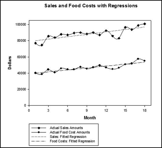
In the real application a formula was used that with hindsight was more complex than it needed to be, and a simpler approach is shown in the next few paragraphs. The result is that locations with food costs that have an increasing percentage are scored as high risk, and locations with a constant or a decreasing food cost percentage are scored as low risk. The food proportions were calculated for each location for each month (food cost divided by sales). The months were numbered 1 to 18. For each location the food proportion was regressed against the period (1 through 18). A positive slope in the regression (called either the slope or b1 in statistics textbooks) would mean that the food proportion was increasing over time. The results are shown in Figure 15.5.
Figure 15.5 The Food Proportion Slopes and Their Risk Scores
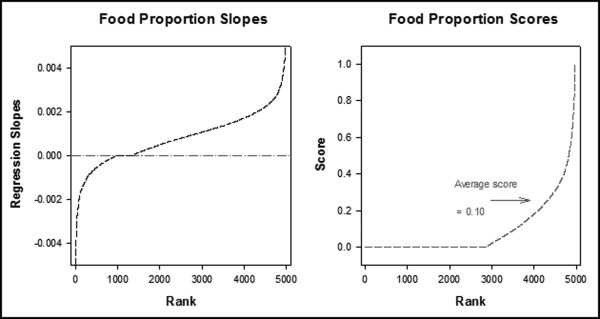
Figure 15.5 shows that about one-fifth of the locations had food proportion slopes that were negative. About 500 locations had food proportion slopes that were zero or near zero. These zero-slope locations included locations with zero sales for any month in the 18-month period because new locations and closed locations have volatile food costs. This left about 70 percent of the locations with positive food proportion slopes where the food costs as a proportion of sales were increasing over the period. P4 was scored as follows:
| Food Proportion Slope | Predictor 4 score |
| Slope > 0.005 | 1 |
| 0.001 ≤ Slope ≤ 0.005 | (Slope −0.001) ∗ 250 |
| Slope < 0.001 | 0 |
The P4 formula gave high scores for high food proportion slopes. A food proportion slope of 0.005 (scored as 1, high risk) means that the food proportion is increasing by about one-half of 1 percent every month for 18 months. A food proportion slope of 0.001 (scored as 0, low risk) means that the food proportion is increasing by about one-tenth of 1 percent every month for 18 months.
P5: Irregular Seasonal Pattern for Sales
P5 uses correlation as discussed in Chapter 13. The logic behind P5 was that sales numbers that deviated from the seasonal patterns were a higher risk for fraud or errors in the reported sales numbers. This predictor is an erratic behavior predictor. For this predictor the criteria is whether the sales numbers followed the seasonal norms. Figure 15.6. shows the typical sales pattern for a calendar year.
Figure 15.6 The Average Sales Pattern Together with the Sales of a Specific Location and a Fitted Regression Line
The left panel of Figure 15.6 shows the annual pattern of sales. The months with seasonally high sales are July, August, and December. February usually has the lowest sales because of winter and because it usually only has 28 days. The right panel of Figure 15.6 is a graph of the sales pattern of a hypothetical restaurant. The sales decrease significantly in the last two months of the year. The correlation between the sales for the specific restaurant and the seasonal pattern is 0.28.
Correlations by themselves are imperfect predictors of fraud risk. The association between underreported sales and a negative correlation is weak (but believed to be strong enough to be included in the risk scoring system), which is why multiple predictors are used in the risk-scoring method. For example, a low correlation matched with an above average increase in sales suggests a low risk of reporting errors. Other predictors, including the trend in sales should be used together with the correlation to the seasonal pattern. The pattern shown on the right hand panel of Figure 15.6 is a high risk situation because of both the low correlation and the sharply decreasing trend. A graph of the ordered correlations and the P5 scores is shown in Figure 15.7.
Figure 15.7 The Correlations and the P5 Scores Applied to the Correlations
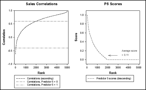
The left-side panel of Figure 15.7 shows the correlations sorted from smallest to largest. The reference lines in the left panel relate to the way that the correlations were scored. Correlations below the lower horizontal reference line were scored as 1.00 (high risk), while correlations above the upper horizontal reference line were scored as 0.00 (low risk). Correlations between the two reference lines were scored with P5 values from 0.00 to 1.00. The P5 scoring formula is as follows:
| Correlation | Predictor 5 score |
| Correlation < −0.4 | 1 |
| −0.4 ≤ Correlation ≤ 0.6 | (Correlation ∗ −1) + 0.6 |
| Correlation > 0.6 | 0 |
In the P5 scoring formula, correlations of 0.6 (and higher) were given a zero score, and correlations of −0.4 (or lower) were scored at 1.00. A correlation midway between −0.4 and 0.6 would be scored at 0.5. The reviews showed that locations on college campuses usually had negative correlations and high P5 scores. This was because July and August were usually low sales months because campuses are usually empty at that time, while February had high sales because the semester was in full swing at that time. A review of the actual sales numbers of locations that scored high on P5 always showed some odd sales pattern meaning that correlation was an effective tool to identify odd sales patterns.
P6: Round Numbers Reported as Sales Numbers
The use of rounded numbers to identify data irregularities was first introduced to the auditing literature in Nigrini and Mittermaier (1997). The predictor P6 was based on the use of round numbers in the reported sales numbers. The assumption was that restaurants that reported round numbers as sales amounts were a higher risk for underreported sales. This predictor is a part of the other special situations group of variables. Round number sales number might be an estimate and might be an indicator of rule-bending by the franchisor. Rule-bending in one area might signal a general disposition towards rules-bending.
The scoring of P6 required a rule as to what numbers constituted round numbers and also what constituted a high count of round numbers. The decision was that a round number would be a number with 0 in the unit position and zero cents after the decimal point. For example, $71,040.00 and $110,460.00 would be round numbers and $22,040.69 and 50,525.00 would not be round numbers. Round numbers ended with 00, 10, 20, . . ., 90 and these 10 two-digit combinations were one-tenth of the possible last two-digit combinations (00, 01, 02, . . ., 99). The expectation was that one-tenth of all reported numbers would be round numbers due purely to chance alone. Under Benford's Law the expected probabilities of the digits tend toward being uniformly distributed when moving from the left to right.
An analysis of the sales numbers showed that about three-quarters of all locations had either 0, 1, or 2 round numbers for the prior 18 monthly sales reports. The expectation was that each location would have 1.8 (one-tenth of 18) round numbers in an 18 month period. The round number counts and the P6 scores are shown in Table 15.4.
Table 15.4 The Distribution of Round Numbers in the Sales Numbers.
| Number of Round Numbers | Proportion | Predictor 6 Score |
| 0, 1, or 2 | 0.764 | 0 |
| 3 | 0.149 | 0 |
| 4 | 0.062 | 0.25 |
| 5 | 0.019 | 0.50 |
| 6 and higher | 0.006 | 1.00 |
A count of either two or three round numbers exceeded the expected value of 1.8, but not by a large margin. Round number counts of four and higher were abnormally high. Only 8.7 percent of the locations had four or more round numbers, and consequently, a positive score for P6. There were not too many positive P6 scores, so the average score was only 0.032.
P7: Repeating Numbers Reported as Sales Numbers
The use of repeated numbers to detect anomalies was introduced to the auditing literature in Nigrini and Mittermaier (1997) as the number duplication test. Because of the seasonal nature of the business, restaurants are unlikely to report exactly the same dollar amount more than once in an 18-month period. This predictor is an other special situations predictor. A location that duplicated a sales number in the past 18 months was seen to be a high risk for fraud or errors. A repeated number might come about when the franchisee reports a number for a prior period in error. In early September the franchisee reports July sales instead of August sales. The July number has already been reported, so the July number will show up as a duplicate.
The average range of the reported numbers was $16,250 over the 18-month period. The difference between the lowest month and the highest month was, on average, $16,250. The chances of an authentic duplicate are very small. The data analysis step for P7 included a calculation of the number of duplicate number locations and the results showed that 106 locations repeated a sales number in the 18-month period. An extract from the duplicate numbers table is shown in Table 15.5.
Table 15.5 An Extract from the Table Showing the Duplicated Sales Amounts.
| Restaurant Number | Amounts Duplicated |
| omitted | $1.00 |
| omitted | $12,239.00 |
| omitted | $27,915.00 |
| omitted | $35,523.00 |
| . . . | |
| omitted | $173,036.00 |
| omitted | $344,986.00 |
The location that duplicated the $1.00 was a college campus location that was closed during July and August. Presumably the owner wanted to report something because the reporting system does not allow sales of zero and so the owner reported $1.00 presumably just to submit a report and to avoid being classified as a nonfiler. A location was given a P7 score of 1.00 if any amount was duplicated during the 18-month period and zero otherwise. The average score for this predictor was very low at 0.02 because duplicates were quite rare.
The franchisor regularly carried out on-site inspections of franchised facilities. These inspections looked at a number of factors related to customer service, hygiene, and operating procedures. The inspection reports ranked the locations (from best to worst) for the current month and for the year to date. This predictor is an other special situations predictor. The logic behind using the inspection rankings was the belief that a franchisee that was conscientious in following the operating procedures to the point of excellence was probably also doing the same with the sales reporting requirements. On the other hand, tardiness in operations was seen to have a high likelihood of spilling over into tardiness in reporting. A high inspection ranking was a sign of a positive attitude towards the franchisor and a desire to have a good relationship.
The score for P8 was based on a weighting of the restaurant's score for the most recent month and the score for the year to date. The P8 scores are shown in Table 15.6.
Table 15.6 The P8 Scores Applied to the Inspection Rankings.
| Inspection Results | Score for V8 |
| Poor scores | 1.0 |
| Worse than average | 0.5 |
| Average | 0 |
| Better than average | 0 |
The scores in Table 15.6 were weighted 2/3 for the year-to-date and 1/3 for the most recent month. The year-to-date inspection scores were believed to be more important than the scores from a single month. A location with no score in the scorecard table was given a score of 1.00 because the lack of any score was seen to be a high-risk situation. The average P8 score was 0.30, which ties in with the fact that only locations with inspection scores that were worse than average were given a P8 score.
This predictor tried to assess whether the franchisor had any pressure to underreport sales. A pressure could exist because the franchisor had a tight cash flow. There was no access to the franchisee's bank details, so an alternate (proxy) predictor was used. It was possible to see how up-to-date the franchisee was with paying the franchise fees. This cash flow predictor is an other special situations predictor that fits in with the pressure aspect of the fraud triangle (pressure, opportunity, and rationalization). P9 was scored based on whether there was a significant overdue balance shown in the accounts receivable listing. The P9 scores are shown in Table 15.7.
Table 15.7 The P9 Scores Applied to the Accounts Receivable Data.
| Description | Score for P9 |
| Significant balance over x days | 1.00 |
| Moderate balance over x days | 0.75 |
| Small balance over x days | 0.50 |
| Zero amount owing over x days | 0.00 |
Table 15.7 shows the scoring formula for P9. If the days' outstanding reference point was (say) 60 days then all locations were tested against having a large, moderate, small, or zero balance that was 60 days overdue. The average score was 0.17, which means that most locations scored a zero for P9.
P10: Use of Automated Reporting Procedures
The company provided an Internet-based reporting system to its franchisees. The system had options for other income sources, sales-related statistics, and permitted deductions. Full compliance was encouraged but was not required by the franchising agreement. The logic behind P10 was that if a franchisee voluntarily used the system and also reported all the small details, then this was a sign of voluntary cooperation and there was a reduced likelihood that the franchisee was engaging in willful sales underreporting. This predictor tried to measure the attitude of the franchisee toward having a cooperative relationship. This predictor is an other special situations predictor. The scoring of P10 took into account (a) whether the franchisee used the system in the immediately preceding month, (b) whether the franchisee had used the system for an extended period, and (c) whether the franchisee reported all or only some of the line-items requested.
The average score for this predictor was 0.38, which again means that the average location scored a zero for this predictor. The average score does not imply that most franchisees people complied perfectly with all information requests, rather it means that locations with below average compliance were given positive scores.
To calculate a final risk score for each location, each of the 10 predictors was weighted with a weighting that ranged from 0.05 to 0.20. Predictors were given low weights if the attributes that they measured were quite rare or if the predictor was seen to have a relatively low predictive ability. Examples of such predictors were P6 round numbers and P7 repeating numbers. A graph of the final risk scores (sorted from largest to smallest) is shown in Figure 15.8.
Figure 15.8 The Final Set of Risk Scores and the Switchboard Control of the System
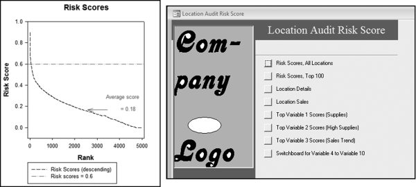
The left side panel of Figure 15.8 is a graph of the final risk scores. The results were very good in that only a small group of about 150 locations had scores that exceeded 0.50, and about 50 locations had scores that exceeded 0.60. The high-scoring locations were the focus of the company's audit efforts for the next year. About 270 locations, or 5.4 percent of the total, had scores of zero, which seems plausible. This means that about 5 percent of all restaurants did not display a single cue associated with a high risk of sales underreporting.
The final scores were compared to those of an earlier pilot study. The correlation between the pilot study risk scores and the current risk scores was 0.15. This means that there was virtually no relationship between the past scores and the current scores. The low correlations were because (a) there were different predictor weights in the current system, (b) the addition of new predictors and the deletion of some of the old predictors, and (c) changed conditions. The low correlation suggests that the risk-scoring system needs to be regularly updated with current data and with other changes that reflect changes in the environment.
An Overview of the Reporting System and Future Plans
An Access database was created for each of the data-cleansing and data-manipulation steps needed to develop the risk-scoring system. The first database was used to import the data into Access and to change layouts and formats as needed. The second database was used for descriptive statistics and the data analysis work needed to calculate what the norms were for each predictor (e.g., the distribution of the food cost percentages). The third database was there for the users. This database calculated the scores for the individual predictors and the final risk score and also produced all the user reports. Several reports were available to the user:
- A report listing the risk scores for all locations.
- A report listing the risk scores of the locations with the 100 highest scores.
- A report for each of the 10 predictors listing the locations that scored high on that predictor only.
- A report where the user could enter a location reference (e.g., 45140) and the final score for that restaurant would be shown together with a list of the scores for that location for each of the 10 predictors. This report showed which predictors contributed the most to the location's overall score.
- An informative report where the user could enter a location number (e.g., 45140) to see the monthly sales history of the location together with other facts and figures related to that location.
The right side of Figure 15.8 shows the opening screenshot (with the company's logo removed) of the system. The system will be updated quarterly with the most recent data. Future system upgrades will probably be based on:
- Changes to the weights of the predictors.
- Changes to the scores associated with the values of the predictors (the equations shown in this chapter).
- Deletion of some predictors and the addition of other predictors.
- The inclusion of prior risk scores as an input to the current risk score.
The inclusion of prior risk scores in the calculation of the current risk score would mean that the risk scoring system has a memory. Prior high scores would linger. A prior score of 0.70 given a weight of 0.20 for the past scores predictor would give the location a starting score of 0.14 in the current period.
Assume that a location shows a large increase in food costs for 2009 to 2010. At the end of 2010 the very high food proportion stabilizes. A large increase in food costs and a large food cost proportion would probably cause the final risk score to be high. By including a prior score in the picture in 2011 we would capture the fact that the food cost percentage recently showed a large increase.
The reported numbers of the highest scoring locations were reviewed as a preliminary evaluation of the system. The highest risk score was 0.897. This location scored 1.00 on all variables except for the round numbers and repeated numbers variables, and marginally less than 1.00 on the sales correlation variable. The restaurant was located near a college, which explains the weak correlation. Colleges have vacations and have fewer people around in July, August, and December.
The round numbers predictor is given a low weight because only a few restaurants have excessive round numbers. However, this predictor is interesting when locations that score high on V6 only are reviewed. The sales numbers of a location with eight round numbers is shown in Table 15.8.
Table 15.8 The Sales Numbers of a Location.
| Month | Sales |
| 1 | 96,907 |
| 2 | 91,537 |
| 3 | 100,920 |
| 4 | 106,640 |
| 5 | 111,242 |
| 6 | 108,740 |
| 7 | 109,159 |
| 8 | 110,035 |
| 9 | 107,762 |
| 10 | 112,012 |
| 11 | 110,300 |
| 12 | 115,070 |
| 1 | 101,850 |
| 2 | 90,908 |
| 3 | 106,252 |
| 4 | 107,539 |
| 5 | 152,390 |
| 6 | 157,780 |
From Table 15.8 it would seem that some level of human intervention was active in the data. The location scored 1.00 on the round numbers predictor, and zero on all the other predictors. It might therefore be that the location is engaged in some innocent rounding and that in all other respects it is a low risk for underreported sales.
The repeating numbers predictor has a low weighting because the repeated numbers incidence is low. The stand-alone results are interesting. One restaurant had two numbers that were each duplicated (a double duplication in the 18-month period). A graph of these values is shown in Figure 15.9 together with the average sales per location.
Figure 15.9 The Sales Numbers of a Location with Sales Duplicates and a High Standard Deviation
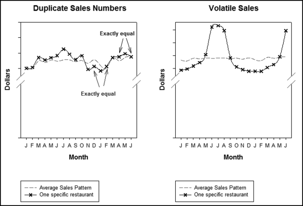
The left-side panel of Figure 15.9 shows the sales pattern of a location that had a double duplication. This location reported the same dollar sales for November and January and the sales for April and June were also equal. The final score for the location was about 0.40, which was higher than the average risk score and placed the restaurant in the seventh percentile. The location scored high on those predictors that related to compliance with policies and procedures (inspections, accounts receivable, and use of the reporting system). This error might be due to reporting sales for the incorrect month.
The right-side graph in Figure 15.9 is a sales pattern that was found as a part of some unstructured exploratory analysis. Locations were ranked by the volatility in their sales. The goal was to see whether a simpler metric would give essentially the same risk rankings. The location has highly volatile monthly sales. The risk score for the location was 0.38, which placed it in the ninth percentile. This risk score was high but an analysis of the data showed that (a) the location was at a seaside resort, which explained the high summer sales and low winter sales, and (b) the largest contributor to the risk score was that the location was not using the internal reporting system. The risk-scoring system painted a far more complete picture of the reporting patterns of the location than would be found by looking at sales volatility only.
The distinction between fraud prevention, which focuses on policies, procedures, training, and communication that stops fraud from occurring, and detection, which comprises activities and programs that detect frauds that have been committed is important. The risk-scoring system is a detection activity. Weaknesses in preventive controls are seen to increase the risk of fraud and place a greater burden on detective controls.
If a risk-scoring system was developed in which the weights of the predictors and the predictors themselves had no relationship to any predictive ability, then the system would function no worse or better than would a random selection of forensic units.
This chapter describes the risk-scoring method and its application to the sales numbers reported by thousands of restaurant franchisees. The risk-scoring method functions well in a continuous monitoring environment. The predictors (of which there were 10 in the franchise application) are indicators of some attribute or behavior of interest. The risk-scoring system was used to detect underreported sales and so the behavior of interest was underreported sales. The risk-scoring predictors could also be called cues or red flags. A forensic unit is the entity or unit that is being scored. Examples could include fast-food restaurants, operating divisions, travel agents, or employees with active purchasing cards. The method works well with scoring hundreds or thousands of forensic units. Based on the numeric values of the predictors, a forensic unit would be seen to have either a low risk of fraud or a high risk of fraud. The final risk score is a score between 0 and 1 reflecting the risk that a forensic unit has engaged in the behavior of interest.
The case study is based on the monthly sales reports of franchisees. The company has only a short window within which to audit the sales numbers before the next wave of sales reports are submitted. The various types of frauds or errors include (a) arithmetic errors, (b) integrity errors (unauthorized deletion of transactions), (c) timing errors (incorrect time period), (d) deliberate fraud, or (e) legal errors (transactions that violate legal clauses) such as omitting nonfood revenues. The cost of a revenue audit by the company's auditors is high. The risk-scoring system was developed to identify high risk sales reports to minimize the costs of auditing locations that were compliant with respect to sales reporting.
The risk scoring system used 10 predictors to identify high-risk forensic units. The 10 predictors were related to (a) high food costs or a food cost percentage that was rapidly increasing, (b) a sales trend that was below average or a pattern of sales numbers that deviated substantially from the usual seasonal pattern, (c) irregularities in the numbers such as round numbers or repeating the same sales number in an 18-month period, (d) noncompliance with other aspects of the franchise agreement as evidenced by weak inspection rankings or incomplete reports submitted through the sales reporting system, or (e) pressure to minimize the franchise fee payments because of cash-flow problems. Each location was scored from 0 to 1 for each predictor. Scores of 1 were associated with a higher risk for sales underreporting.
For the final risk score, the predictors were weighted according to their importance and the final score was a weighted sum of the scores on the individual predictors. The locations with the highest final scores were the targets of franchise audits. The chapter included some of the future plans for improvements to the system. The logic and methodology could be adapted to other forensic analytic environments in which auditors or management wanted a formal system to evaluate the risk of a specific type of intentional or unintentional errors. The next chapter describes other examples and programming issues that need to be considered when using Access to program the system. The common thread in the applications is that the behavior of interest is very specific and the goal is a small set of audit targets that are a high risk for fraud or errors.