Chapter 7
Benford's Law
The Second-Order and Summation Tests
Chapters 5 and 6 dealt with forensic analytic situations where we expected our data to follow Benford's Law. Those chapters included guidelines for assessing which data sets should follow Benford's Law and a review of methods for measuring conformity to Benford's Law. In contrast, this chapter deals with two Benford's Law tests that do not rely on the data conforming to Benford's Law. One of these tests is called the second-order test. This relatively new test can be applied to (almost) any set of data. The second-order test looks at relationships and patterns in data and is based on the digits of the differences between amounts that have been sorted from smallest to largest (ordered). The digit patterns of the differences are expected to closely approximate the digit frequencies of Benford's Law. The second-order test gives few, if any, false positives in that if the results are not as expected (close to Benford), then the data do indeed have some characteristic that is rare and unusual, abnormal, or irregular.
The second of these new tests is called the summation test. The summation test looks for excessively large numbers in the data. The summation test is an easy extension to the usual first-two digits test and it can be run in either Access or Excel. This chapter also introduces Minitab as a possible tool for forensic analytics. The second-order test uses some of the mathematics from the prior chapter. The summation test uses some of the logic from Chapter 5. Both the second-order tests and the summation tests are run on the first-two digits. As is usual for the Benford's Law tests, the tests are run on the entire data table. Data is only ever sampled as a work-around to graphing a data table to stay within Excel's graphing limit of 32,000 data points.
A Description of the Second-Order Test
A set of numbers that conforms closely to Benford's Law is called a Benford Set. The link between a geometric sequence and a Benford Set is discussed in the previous chapter. The link was also clear to Benford who titled a part of his paper “Geometric Basis of the Law” and declared that “Nature counts geometrically and builds and functions accordingly” (Benford, 1938, 563). Raimi (1976) relaxes the tight restriction that the sequence should be perfectly geometric, and states that a close approximation to a geometric sequence will also produce a Benford Set. Raimi then further relaxes the geometric requirement and notes that, “the interleaving of a number of geometric sequences” will also produce a Benford Set. A mixture of approximate geometric sequences will therefore also produce a Benford Set. This equation for a geometric sequence, Sn, is given in the prior chapter and is restated here again for convenience:
where a is the first term in the sequence, r is the common ratio of the (n+1)st element divided by the nth element, and n denotes the nth term. In a graph of a geometric sequence (see Figure 5.1), the rank (1, 2, 3, . . ., N) is shown on the x-axis, and the heights on the y-axis are arn-1.
The digits of a geometric sequence will form a Benford Set if two requirements are met. First, N should be large and this vague requirement of being “large” is because even a perfect geometric sequence with (say) 100 records cannot fit Benford's Law perfectly. For example, for the first-two digits from 90 to 99, the expected proportions range from 0.0044 to 0.0048. Because any actual count must be an integer, it means that the actual counts (either 0 or 1) will translate to actual proportions of either 0.00 or 0.01. As N increases the actual proportions are able to tend toward the exact expected proportions of Benford's Law. Second, the difference between the logs of the largest and smallest numbers should be an integer value. The geometric sequence needs to span a large enough range to allow each of the possible first digits to occur with the expected frequency of Benford's Law. For example, a geometric sequence over the range [30, 89.999] will be clipped short with no numbers beginning with a 1, 2, or a 9.
The remainder of the discussion of the second-order test draws on Nigrini and Miller (2009). The algebra below shows that the differences between the successive elements of a geometric sequence give a second geometric sequence Dn of the form
where the first element of the sequence is now a(r−1), and r is still the ratio of the (n + 1)th element divided by the nth element. Since the elements of this new sequence form a geometric series, the distribution of these digits will also conform to Benford's Law and the N − 1 differences will form a Benford Set.
The second-order test of Benford's Law is based on the digit patterns of the differences between the elements of ordered data and is summarized as follows:
- If the data is made up of a single geometric sequence of N records conforming to Benford's Law, then the N − 1 differences between the ordered (ranked) elements of such a data set gives a second data set that also conforms to Benford's Law.
- If the data is made up of nondiscrete random variables drawn from any continuous distribution with a smooth density function (e.g., the Uniform, Triangular, Normal, or Gamma distributions) then the digit patterns of the N − 1 differences between the ordered elements will be Almost Benford. Almost Benford means that the digit patterns will conform closely, but not exactly, to Benford's Law.
- Some anomalous situations might exist when the digit patterns of the differences are neither Benford nor Almost Benford. These anomalous situations are expected to be rare. If the digit patterns of the differences is neither Benford nor Almost Benford it is an indicator that some serious issue or error might exist in the data.
Miller and Nigrini (2008) describe and develop the mathematical proofs related to the second-order test. One odd case where the differences do not form a Benford Set exists with two geometric sequences where, for example, N1 spans the [30,300) interval and the second geometric sequence N2 spans the [10,100) interval. The combined sequence therefore spans the range [10,300). The differences between the elements do not conform to Benford's Law even though the digit frequencies of the source data (N1 and N2) both individually and combined (appended) all conform perfectly to Benford's Law. The differences between the ordered elements of the two geometric sequences when viewed separately also form Benford Sets. However, when the two sequences are interleaved, the N1 + N2 − 1 differences do not conform to Benford's Law. This odd situation would be rare in practice.
The differences are expected to be Almost Benford when the data is drawn from most of the continuous distributions encountered in practice. A continuous distribution is one where the numbers can take on any value in some interval. To formally describe these differences, let Y1 through Yn be the Xi's arranged in increasing order (Y1 is the smallest value and Yn the largest); the Yi's are called the order statistics of the Xi's. For example, assume we have the values 3, 6, 7, 1, and 12 for X1 through X5. Then the values of Y1 through Y5 are 1, 3, 6, 7, and 12, and the differences between the order statistics are 2, 3, 1, and 5. The second-order Benford test is described as follows:
Let x1, . . ., xN be a data table comprising records drawn from a continuous distribution, and let y1, . . ., yN be the xi's in increasing order. Then, for many data sets, for large N, the digits of the differences between adjacent observations (yi+1 – yi) is close to Benford's Law. A pattern of spikes at 10, 20, . . ., 90 will occur if these differences are drawn from data from a discrete distribution. Large deviations from Benford's Law indicate an anomaly that should be investigated.
Since most distributions satisfy the conditions stated above, the expectation is that we will see Almost Benford results from most data tables. There is only a small difference between the Benford and Almost Benford probabilities, and these differences depend only slightly on the underlying distribution. The suggested approach to assessing conformity in the second-order test is to either look at the data and make a subjective judgment call, or to use the mean absolute deviation (MAD). The formal tests such as Z-statistics, the chi-square test, or the K-S test are not appropriate because we will usually be dealing with large data sets and the expectation is Almost Benford, so we are not even expecting exact conformity.
To demonstrate Almost Benford behavior, the results of four simulations from very different distributions are shown. The data was simulated in Minitab 16 using the Calc→Random Data commands. The numbers in fields C1, C3, C5, and C6 were then sorted using Data→Sort. The differences between the numbers were calculated using Calc→Calculator.
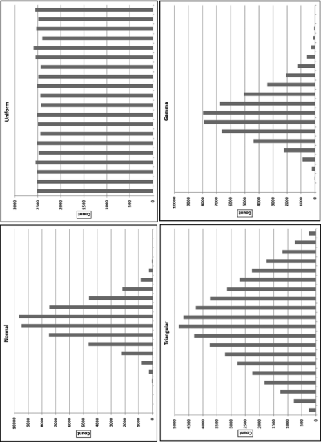
The simulated data and the calculated differences are shown in Figure 7.1. The next step was to prepare histograms of the four data sets to see how different the distributions actually are. The four histograms in Figure 7.2 show (a) a normal distribution with a mean of 5000 and a standard deviation of 1000, (b) a uniform distribution over the [0,10000) interval, (c) a triangular distribution with a lower endpoint of 0 and an upper endpoint of 10000 and a mode of 5000, and (d) a Gamma distribution with a shape parameter of 25 and a scale parameter of 5000. Each of the data tables had 50,000 records. The four distributions in Figures 7.1 and 7.2 were chosen so as to have a mixture of density functions with positive, zero, and negative slopes as well as a combination of linear and convex and concave sections in the density functions. The scale parameters (the means) have no effect on the differences between the ordered records. The shape parameters (the standard deviations) do impact the sizes of the differences, as do the number of records (N). The four histograms are shown in Figure 7.2.
Figure 7.1 The Minitab Calculations for the Second Order Test
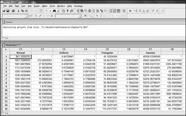
Figure 7.2 The Histograms of Four Simulated Data Tables of 50,000 Records Each
The next step in the second-order test was to analyze the digit patterns of the differences between the ordered (ranked) amounts for each distribution. Because each data table had 50,000 records there were 49,999 differences per data table. In Figure 7.1 the first three differences for the normal distribution in column C2 are 212.656, 27.908, and 31.856. The differences for the other distributions are in columns C4, C6, and C8. Before calculating the first-two digits for each table of differences, the smallest difference was calculated for each table. These minimums were 0.00000021, 0.00000013, 0.00000807, and 0.00001013 respectively. Each of the difference amounts (in all four columns) was multiplied by 100,000,000 if the amount was less than 1.00, so that all numbers had two digits to the left of the decimal point (0.00000021∗100000000 equals 21.0). The four differences columns were then imported into Access. The first-two digits queries (see Figures 5.3 and 5.4) were run and the graphs were prepared. The results for each data table are shown in Figure 7.3.
Figure 7.3 The First-Two Digits of the Differences
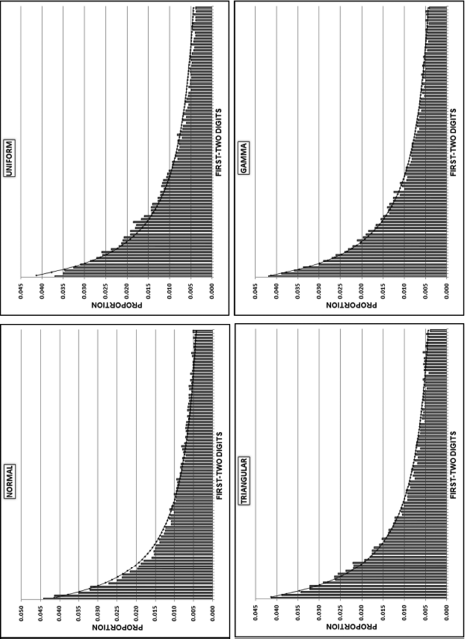
The first-two digits of the differences, hereinafter called the second-order test, are all Almost Benford despite the fact that their densities in Figure 7.2 have completely different shapes. Almost Benford means that in one or two sections of the graph the actual proportions will tend to be less than those of Benford's Law, and in one or two sections the actual proportions will tend to exceed those of Benford's Law. The “over” and “under” sections are easier to see with larger data sets but we generally have either two “over” sections and one “under” section, or two “under” sections and one “over” section. If the simulations were repeated with larger data sets and the results aggregated, then these “over” and “under” sections would be easier to see. The differences between the ordered records of numbers drawn from a continuous distribution will exhibit Almost Benford behavior, but they will seldom conform perfectly to Benford's Law even with N tending to infinity (Miller and Nigrini, 2008). These differences should be close to Benford's Law for most data sets, and an analysis of the digits of the differences could be used to test for anomalies and errors. What is quite remarkable is that when all four data tables of 49,999 differences were appended to each other (to create one big data table of 199,996 records) the large data table had a MAD of 0.000294, which according to Table 6.1 is close conformity.
Running the Second-Order Test in Excel
The second-order test was run on the InvoicesPaid data set from Chapter 4. The data profile showed that there were 189,470 invoices. The first-order test in Chapter 5 showed that the data did not conform to Benford's Law using the traditional Z-statistics and chi-square tests. However, there was the general Benford tendency in that the low digits occurred more frequently than the higher digits. Again, the second-order test does not require, or assume, conformity to Benford's Law. This test is usually run on all the numbers (including negative numbers and small positive numbers).
The second-order test cannot be run in Access. Access cannot easily calculate the differences between the sorted records. So if the 1,000th record was for $2,104 and the 1,001st record was for $2,150, Access cannot easily calculate that the difference is $46. This is because of the database concept that both row order and column order are unimportant in the design of tables in relational databases. Access has a domain aggregate function called DLookUp. The DLookUp function can be used to show the Amount from the preceding row. These domain aggregate functions are slow to execute and are impractical with large tables. The suggested approach is to use Excel to sort the records and to calculate the differences. Another approach would be to use IDEA, which includes the second-order test as a built-in routine.
The procedure in Excel would be to use the NigriniCycle.xlsx template and to sort the Amount ascending. The sort is done using Home→Editing→Sort&Filter→Custom Sort.
Figure 7.4 The Sort Procedure Used to Start the Second-Order Test
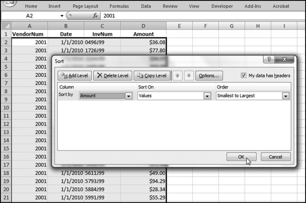
The sort procedure is shown in Figure 7.4. Click OK to sort the Amount field from smallest to largest. The next step is to create a new field, which we call Diffs (for differences) in column F. The blank column E is there to have a dividing line between our source data and our calculated values. The formula for the calculation of the differences for cell F3 is,
F3: = (D3−D2) * 1000
The multiplication by 1,000 is so that amounts such as 0.01 become 10.00 and we can then use the Left function to calculate the first-two digits. The formula needs to be copied down to the last row of the data. The next step is to format column F as Currency. We will always have one blank (null) cell because a data set with N records only gives us N − 1 differences. The next step is to calculate the first-two digits of each difference in column G. The formula in cell G3 is,
G3: = VALUE(LEFT(ROUND(F3,0),2))
The ROUND function is to be sure that we get the correct first-two digits. Excel might store a number such as 20 as 19.99999999999, which is fine for most calculations, except to identify the first-two digits. The comma 2 in the LEFT function indicates that we want the leftmost two digits. The VALUE part of the function means that we want the result as a number. The results are shown in Figure 7.5.
Figure 7.5 The Calculation of the First-Two Digits of the Differences
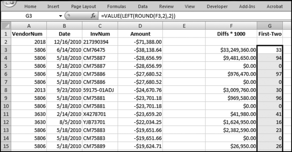
The calculation of the digits of the differences is shown in Figure 7.5. The next step is to count how many of the differences have 10, 11, 12, and so on as their first-two digits. In Access this would be a Group By query. In Excel this task is done with the COUNTIF function in the Tables worksheet. The COUNTIF formula in cell J3 of the Tables worksheet is

The formula essentially looks at the first-two digits calculations in the Data worksheet and counts all the occurrences of 10, 11, 12, and so on. The reference to cell I3 is to the number 10 in I3 and cell J3 counts the number of 10s. When the formula is copied down to cell J92 the counts are for the numbers 10, 11, 12, and so on to 99. The results are shown in Figure 7.6.
Figure 7.6 The Results of the Second-Order Test
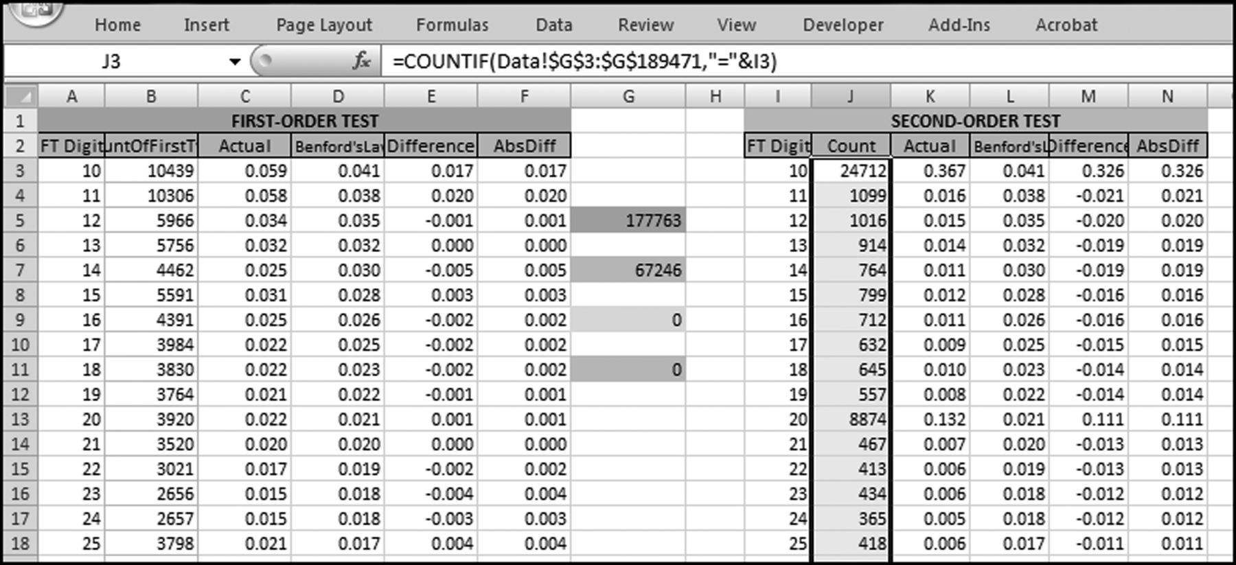
The NigriniCycle.xlsx template works in much the same way as for the first-order test. The record count for the second-order test is shown in cell G7 in the Tables worksheet. Since the original data table had 189,470 records we expect 189,469 (N − 1) differences. We only have 67,246 numbers with valid digits because the data table contained excessive duplication and there are only 67,247 different numbers being used in the data table of 189,470 records. When two successive numbers are equal (e.g., 50.00 and 50.00) then the difference between these numbers is zero and zero is ignored in the analysis of the digits of the differences. The excessive duplication will be clearer from the first-two digits graph. The graph is prepared in the template and can be seen by clicking on the SecondOrder tab.
Figure 7.7 The Second-Order Test of the Invoices Data
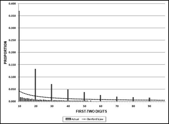
The result of the second-order test of the InvoicesPaid data is shown in Figure 7.7. The first-order result in Chapter 5 showed five large spikes, and aside from that, the fit was at least reasonable from a visual perspective. For most of the higher first-two digit combinations (51 and higher) the difference between the actual and expected proportions was only a small percentage. The InvoicesPaid data did not conform using the conformity criteria. The deviations are comparable to those of the accounts payable data analyzed in Nigrini and Mittermaier (1997).
The results of the second-order test in Figure 7.7 are based on 67,246 nonzero differences. Differences of zero (which occur when the same number is duplicated in the list of ordered records) are not shown on the graph. The second-order graph in Figure 7.7 seems to have two different functions. The first Benford-like function applies to the first-two digits of 10, 20, 30, . . ., 90, and a second Benford-like function applies to the remaining first-two digit combinations (11 to 19, 21 to 29, . . ., 91 to 99). The groups are called the prime and the minor first two-digits:
1. Prime: First-two digits: 10, 20, 30, 40, 50, 60, 70, 80, and 90. d1d2 mod 10 = 0
2. Minor: First-two digits: 11, 12, 13, . . ., 19, 21, 22, 23, . . ., 29, 31, . . ., 99. (d1d2 mod 10 ≠ 0)
The InvoicesPaid numbers are tightly clustered. For example, there were 139,105 records with an Amount field from $10.00 to $999.99. There are 99,000 different numbers from 10 to 999.99. A test showed that 39,897 of the available numbers between 10 and 999.99 were used. This suggests that the differences between the numbers in the 10 to 999.99 range are generally small and are probably 0.01, 0.02, and 0.03. Another test showed that there are 21,579 differences of 0.01, 7,329 differences of 0.02, and 3,563 differences of 0.03. The decrease in the counts is dramatic and there are only 464 differences of 0.08. The largest difference in this range is 0.47. The numbers in the 10 to 999.99 range are indeed tightly packed.
A difference of 0.01 has first-two digits of 10 because this number can be written as 0.010. A difference of 0.02 has first-two digits of 20 because 0.02 can be written as 0.020. The reason for the prime spikes in Figure 7.7 is that the numbers are tightly packed in the $10.00 to $999.99 range with almost three-quarters of the differences being 0.01 or 0.02. The mathematical explanation for the systematic spikes on the prime digits is that the InvoicesPaid table is not made up of numbers from a continuous distribution. Currency amounts can only differ by multiples of $0.01. The second-order results are caused by the high density of the numbers over a short interval and because the numbers are restricted to 100 evenly spaced fractions after the decimal point. The prime spikes should occur with any discrete data (e.g., population numbers) and the size of the prime spikes is a function of both N and the range. That is, we will get larger prime spikes for larger data tables with many records packed into a small range. This pattern of spikes does not indicate an anomaly; it is a result of many numbers restricted to being integers or to fractions such as 1/100, 2/100, 3/100 being fitted into a tight range that restrict the differences between adjacent numbers.
An Analysis of Journal Entry Data
The next case study is an analysis of the 2005 journal entries in a company's accounting system (the second-order test was not known at the time). The external auditors did the usual journal entry tests, which comprised some high-level overview tests for reasonableness (including Benford's Law), followed by some more specific procedures as required by the audit program. The journal entries table had 154,935 records of which 153,800 were for nonzero amounts. The dollar values ranged from $0.01 to $250 million and averaged zero since the debits were shown as positive values and the credits as negative values. The dollar values were formatted as currency with two decimal places. The results of the first-order test are shown in Figure 7.8.
Figure 7.8 The First-Order Results for the Corporate Journal Entries
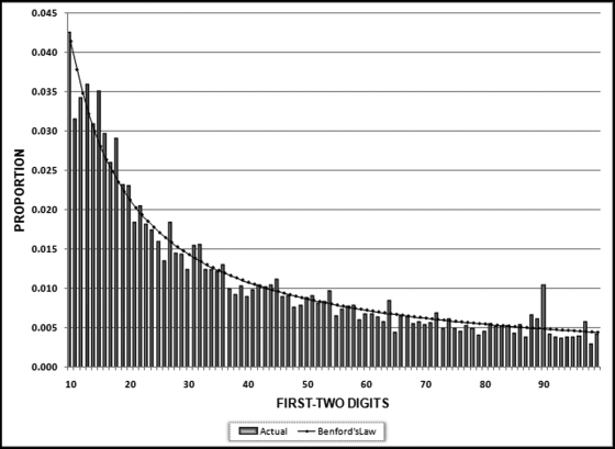
The results show a reasonable conformity to Benford's Law as would be expected from a large collection of transactional data. The calculated MAD was 0.001163, which just squeaks in with a “close conformity” score using Table 6.1. There is a spike at 90, and a scrutiny of the actual dollar amounts (e.g., 90.00, 9086.06) reveals nothing odd except for the fact that 111 amounts with first-two digits of 90 were for amounts equal to 0.01. The reason for this will become clear when the second-order results are discussed. The second-order results are shown in Figure 7.9.
Figure 7.9 The Second-Order Results for the Corporate Journal Entries
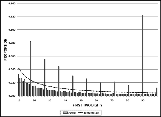
The second-order test results in Figure 7.9 show that there are anomalous issues with the data. First, there is no spike at 10 and a large spike is expected for data representing dollars and cents in tightly clustered data due to differences of 0.01, which have first-two digits of 10 (since 0.01 is equal to 0.010). Second, there is a large spike at 90 and while spikes are expected at the prime digits, the largest of these is expected at 10 and the smallest at 90. Third, there is an unusual spike at 99. The 99 is a minor combination and 99 has the lowest expected frequency for both the first-order and second-order tests.
Further work showed that while the data was formatted as currency with two digits to the right of the decimal point (e.g., $11.03), there were amounts that had a mysterious nonzero third digit to the right of the decimal point. The extra digits can be seen if the data is formatted as a number with three digits to the right of the decimal point. A data extract is shown in Figure 7.10.
Figure 7.10 A Sample of the Journal Entry Data
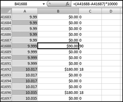
The journal entry data was originally housed in an Access database. The data was imported into the NigriniCycle.xlsx template using Excel's data import function. The import function is activated using Data→Get External Data→From Access. The file and the specific table are then selected. This method is better than using the clipboard, which is limited in size. Using this data import method causes the rows to be shaded and the original Access formatting is lost (which helped to see the data issue).
Transactional data can have a third digit as long as the third digit is a zero. For example, 11.030 can be shown as $11.03. To evaluate how many times a nonzero third digit occurred, all amounts were multiplied by 100 and the digits to the right of the decimal point were analyzed. Approximately one-third of the amounts in the data table had a digit of zero to the right of the decimal point. The digits 1 through 9 appeared to the right of the decimal point with an average frequency of 7.3 percent and the percentages ranged from 6.2 percent for the digit 3 to 8.4 percent for the digit 2.
Follow-up work was done to see whether the extra digit occurred more frequently in any particular subset of the data, but the extra digit occurred with an almost equal frequency across the four quarters that made up the fiscal year. No systematic pattern was evident when the data was grouped by source (a field in the table). The proportion of numbers with third digits was about the same for the four largest sources (payroll, labor accrual, spreadsheet, and XMS).
The third digit explains why amounts displayed as $0.01 were shown to have first-two digits of 90. This was because unformatted numbers of 0.009 rounded to $0.01 when formatted as currency. In the journal entry data the second-order test showed a data inconsistency that was not apparent from the usual Benford's Law tests and also not apparent from any other statistical test used by auditors. While the dollar amounts of the errors were immaterial and did not affect any conclusions reached, this might not be the case for data that could be required to be to a high degree of accuracy.
The second-order test is a recent development. With the second-order test the data can contain errors and anomalies and we would still expect the second-order results to approximate Benford's Law. We can therefore get “good” results (such as Figure 7.3 or Figure 7.7) from bad data. On the other hand, when the second-order test signals an issue (because it is neither Almost Benford nor does it have the pronounced spikes at the prime digits) then the data really does have some issue. Simulations have shown that the test can detect excessive rounding (these results will look just like Figure 7.7 though). In another simulation the second-order test was run on data that was not ranked in ascending order. The situation could be where the investigator was presented with data that should have a natural ranking such as the number of votes cast in precincts ranked from the earliest report to the last to report, or miles driven by the taxis in a fleet ranked by gasoline usage. The second-order test could be used to see whether the data was actually ranked on the variable of interest. The general rule is that if the data is not correctly sorted then the second-order results will not be Almost Benford.
The summation test has been dormant for nearly 20 years and it is time to put it to good use. Benford's Law is based on the counts of the number of numbers with first-two digits 10, 11, 12, . . ., 99. In contrast, the summation test is based on sums rather than counts. The summation test seems particularly useful when viewed in the light of an article in the Wall Street Journal (1998):
Kenneth L. Steen of Chattanooga, Tenn., was expecting a $513 tax refund. Instead he got a letter from the Internal Revenue Service informing him that he owes the government $300,000,007.57. “It's mind-boggling,” Mr. Steen says. “I thought they had become the new, friendlier, more efficient IRS, and then this happens.” Mr. Steen has plenty of company. An IRS official says about 3,000 other people around the nation got similar erroneous notices, each showing a balance-due of “three hundred million dollars and change.”
The important facts are that all the erroneous amounts had first-two digits of 30 and all the amounts are very large when compared to normal balance-due notices. The Treasury is a bit lucky that the errors were balance-due notices and not taxpayer refunds. Had the Treasury issued 3,000 treasury checks for $300 million each it is quite possible that they would still be looking for some of the taxpayers and their money! To get an idea of just how big these erroneous amounts are, we could sum all 3,000 of the $300 million errors. The answer would be an amount equal to approximately 10 percent of the Gross Domestic Product of the United States of America (in 1998, which was when the error occurred). It is surprising that an accounting error equal to 10 percent of GDP was not detected internally prior to the notices being sent out to taxpayers.
With about 125 million tax returns per year an additional 3,000 amounts with first-two digits 30 would probably not cause anything resembling a spike on the IRS's first-two digits graph. Using the expected probability of the 30 we would expect about 1.8 million tax returns to have a balance-due or a refund amount with first-two digits of 30. An increase to 1.83 million would not affect the graph even slightly if we only compare a count of 1.80 million to 1.83 million. The ability to detect the errors improves dramatically of we look at the sum of these numbers.
I developed the summation theorem as a Ph.D. student. I still remember walking home from classes one day and asking myself what the relationship was between the sums of all the numbers with first-two digits 10, 11, 12, . . ., 99 in a Benford Set. Do the sums have the same pattern as the counts? It did not take long to simulate a synthetic Benford Set and then to calculate the sums. I was quite surprised by the result that the sums were approximately equal. The proof and the underlying mathematics require a little calculus as is shown in Equation 7.3.
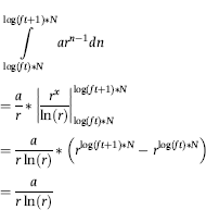
The first line of the equation calculates the area under the curve for an unspecified first-two digit combination abbreviated ft. The number of records is N, and the function is the sequence described by Equation 7.1. To keep the sequence neat we can restrict a to being equal to 10k with k ≥ 0, and k integer. This means that the starting point will be 10, or 100, or 1,000 or some similarly neat number. In the last step, the entire second term disappears. This is because of a neat substitution of 10(1/N) for r (as in Equation 6.14), which makes the second term equal to (1 − 0) or 1, and a “multiplication by 1” term can be dropped in the equation. In this example the log of the upper bound (say 100) minus the log of the lower bound (say 10) equals 1. This simplifies the mathematics above and the result can be generalized to cases where the difference between the logs exceeds 1.
The implication of ft disappearing from Equation 7.3 tells us that the areas under the curve do not depend on which first-two digits we are talking about. The areas under the curve are independent of ft and this means that they must be equal.
As a test of the mathematics we will create a synthetic Benford Set of 20,000 records with a lower bound of 10 and an upper bound of 1,000, just to make things a little more complex than Equation 7.3. We do not want too few records in the data table because the pattern will then not be clear. Also, too many records will make the pattern too neat. We will follow the logic in equations 6.12, 6.13, and 6.14, and Figure 6.8. We need to calculate the value of r that will give us a geometric sequence from 10 to 1,000 with N = 20,000 using Equation 6.14.
We will use the Data worksheet in the NigriniCycle.xlsx template to create our synthetic Benford Set.
Figure 7.11 The Synthetic Benford Set with 20,000 Records
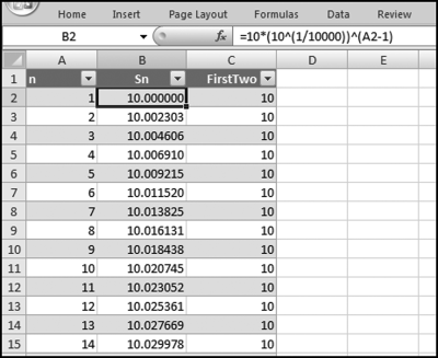
The data table that will be used for the summation test is shown in Figure 7.11. The formula in cells B2 and C2 are,
B2: = 10*(10ˆ(1/10000))ˆ(A2−1)
C2: = VALUE(LEFT(B2,2)) (first-two digits calculation)
In the geometric sequence in column B we have a equal to 10 (the starting value) and the common ratio r equal to 10(1/10000). The B2 and C2 formulas are copied down to row 20001. There are 20,000 records and one row is used for headings. The next step is to calculate the sums in the Tables worksheet. The formula and the results are shown in Figure 7.12.
Figure 7.12 The Calculated Sums of the Summation Test
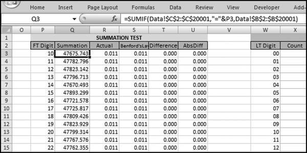
The summation test's sums are calculated in column J of the Tables worksheet. The formula for column J is shown below.
J5: = SUMIF(Data!$C$2:$C$20001,” = “&P3,Data!$B$2:$B$20001)
The first term in the formula states the column that we are filtering on. The second term is our condition (which is to equal 10, 11, or 12, or whatever the case may be). The third term is the range that we want to add (sum).
For the summation test all the Benford's Law proportions are equal amounts because we expect the sums to be equal. Also, the 90 possible (equal) proportions must add up to 1.00 because every valid number has a first-two digit combination. The expected sum stated as a proportion for the first-two digits is equal to 1/90. The summation graph is automatically prepared in the template and it can be seen by clicking on the Summation chart sheet.
Figure 7.13 The Results of the Summation Test on a Benford Set of 20,000 Records
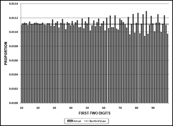
The summation test results are shown in Figure 7.13. The bars are all very close to the expected values of 0.0111. Some variability can be seen as we move from left to right. This is because the actual and expected counts are lower for the higher digits and sometimes the simulation generates slightly fewer than expected or slightly more than expected records with a (say) first-two digits of 85. Since we are dealing with sums it looks like a large effect. Also, note the calibration of the y-axis where the minimum value is 0.01 and the actual sums are actually all close to the 0.111 expectation.
Running the Summation Test in Access
For the summation test the calculations could be done in Access but the graph still needs to be prepared in Excel. The steps for the InvoicesPaid data are shown. The first stage (or step) is to make a table that includes only the positive amounts. No other fields are needed in the table. The table is created with the query shown below and the >0 criteria for the field named PosAmount. The Make Table query is created by selecting Make Table in the Query Type group. Enter the table name as tblPosAmounts. Click OK. Click Run.
Figure 7.14 The Make Table Query Used to Create a Table of the Positive Amounts
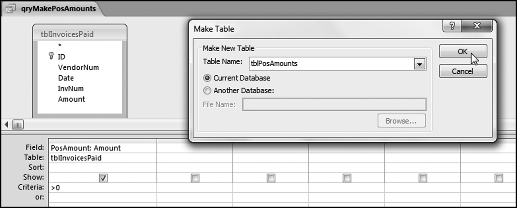
The query used to create a table of the positive invoice amounts is shown in Figure 7.14. Click Yes after the warning that you are about to paste 185083 rows into a new table. At this stage we could import the data into Excel and then use the NigriniCycle.xlsx template because the table has less than 1,048,576 records. Note that in Excel we would not simply use the LEFT function because the leftmost two characters of 4.21 are “4.” We would have to use LEFT(B2∗1000,2) for the first-two digits and then we would have to look for accuracy issues (where 20 is perhaps held in memory as 19.99999999). It is easier to do the summation calculations in Access. The query to calculate the first-two digits is shown in Figure 7.15.
Figure 7.15 The Query Used to Calculate the First-Two Digits of Each Amount
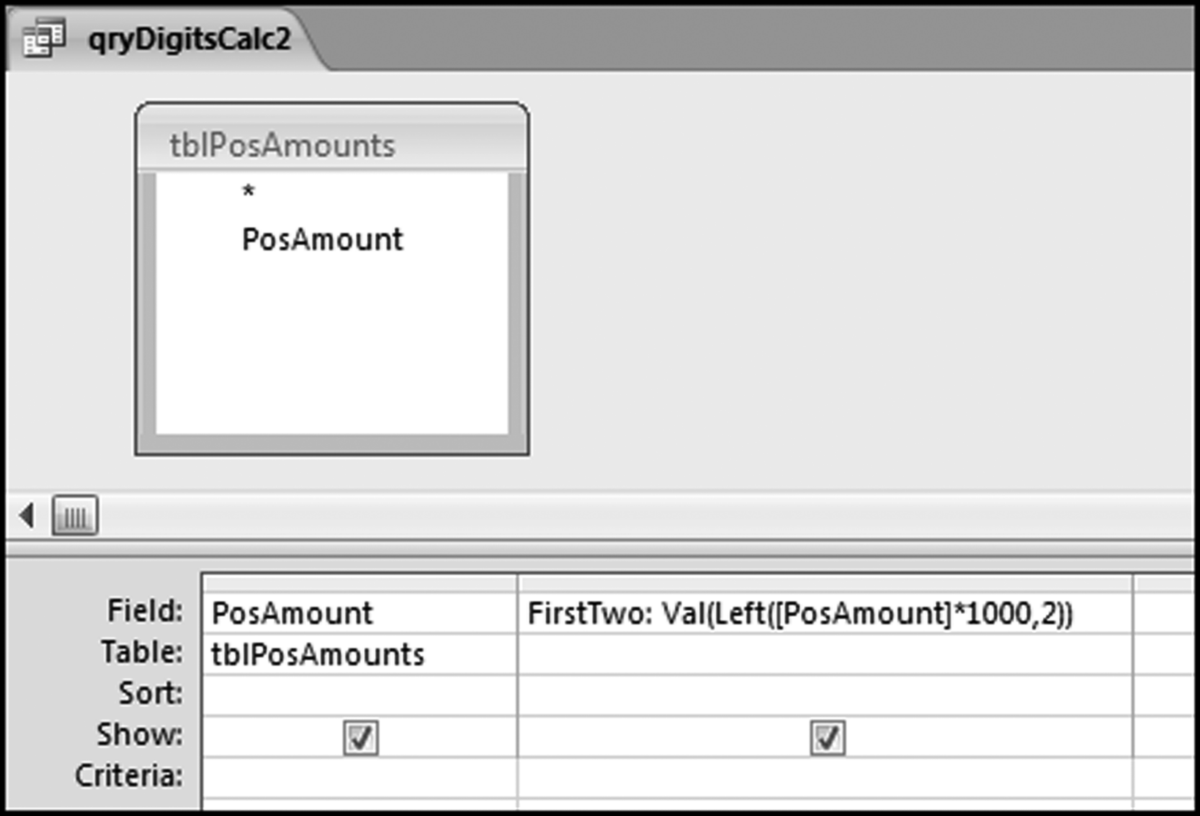
This query is similar to the usual query for the first-order test except that the query is run against all positive amounts. The formula in qryDigitsCalc2 is,
FirstTwo:Val(Left([PosAmount]*1000,2))
The second query calculates the required sums of the numbers. This query differs from the query used in the first-order test.
Figure 7.16 Shows the Query Used to Calculate the Sums of the Amounts
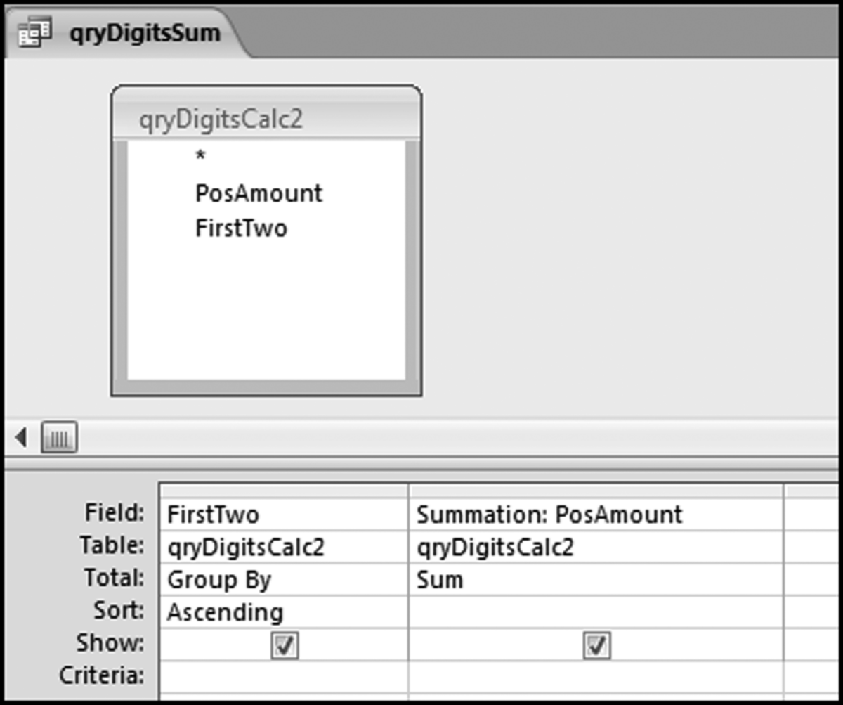
The second summation test query is shown in Figure 7.16. The first-order test counts the amounts whereas the summation test sums the positive amounts. The sums are grouped by the first-two digits. The result can be copied and pasted using Copy and Paste into the NigriniCycle.xlsx template also using column Q as is shown in Figure 7.12. The summation graph can be accessed by again simply clicking on the Summation chart sheet. The results are shown in Figure 7.17.
Figure 7.17 The Results of the Summation Test for the Invoices Data
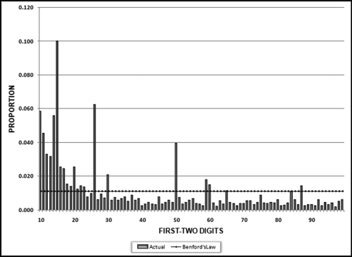
The summation graph shows little conformity to Benford's Law. The graph shows that we have an excess of large numbers with first-two digits 10, 11, 14, 15, 26, and 50. These results will be investigated further in Chapter 8.
Experimentation with the summation theorem has shown that real-world data sets seldom show the neat straight-line pattern shown on the graph even though this is the correct theoretical expectation. This is because in the real world we do have abnormal duplications of large numbers. At this stage we cannot say whether the spikes are caused by a handful (one, two, or three) of very big numbers or an abnormal duplication of a few hundred moderately big numbers. The usual Benford's Law result in Chapter 5 had spikes at 10, 11, 50, 98, and 99, indicating high counts for these digit combinations. This suggests that the numbers at 98 and 99 are small because they do not affect the summation result. The numbers at 10, 11, and 50 are moderately large because the count and the sums are high. The numbers for 14, 15, and 25 are probably very large because they affect the summation, but not the graph based on the counts. This is a new test and results, findings, and comments from users are welcomed.
Discussion
The second-order test analyses the digit patterns of the differences between the ordered (ranked) values of a data set. In most cases the digit frequencies of the differences will closely follow Benford's law irrespective of the distribution of the underlying data. While the usual Benford's Law tests are usually only of value on data that is expected to follow Benford's law, the second-order test can be performed on any data set. This second-order test could actually return compliant results for data sets with errors or omissions. On the other hand, the data issues that the second-order tests did detect in simulation studies (errors in the download, rounding, and the use of statistically generated numbers) would not have been detectable using the usual Benford's Law tests.
The second-order test might be of use to internal auditors. In ACFE, AICPA, & IIA (2008) the document focuses on risk and the design and implementation by management of a fraud risk program. It is important to distinguish between prevention, which focuses on policies, procedures, training, and communication that stops fraud from occurring, and detection, which comprises activities and programs that detect frauds that have been committed. The second-order test would be a detection activity or detective control.
ACFE, AICPA, & IIA (2008) notes that a “Benford's Law analysis” can be used to examine transactional data for unusual transactions, amounts, or patterns of activity. The usual suite of Benford's Law tests are only valid on data that is expected to conform to Benford's Law whereas the new second-order test can be applied to any set of transactional data. Fraud detection mechanisms should be focused on areas where preventive controls are weak or not cost-effective. A fraud detection scorecard factor is whether the organization uses data analysis, data mining, and digital analysis tools to “consider and analyze large volumes of transactions on a real-time basis.” The new second-order and summation tests should be included in any suite or cycle of data analysis tests.
In a continuous monitoring environment, internal auditors might need to evaluate data from a continuous stream of transactions, such as the sales made by an online retailer or an airline reservation system. Unpublished work by the author suggests that the distribution of the differences (between successive transactions) should be stable over time and consequently the digits of these differences should also be stable across time. Auditing research could address how the second-order test could be adapted so that it analyzes the differences between successive transactions. Future research that shows potential benefits of continuously running the second-order tests on the differences between the (say) last 10,000 records of transactional data might be valuable. Such research could show what patterns might be expected under conditions of “in control” and “out of control.” Research on the detection of anomalies is encouraged given the large penalties for external audit failures.
This chapter introduced two new reasonably advanced forensic analytic tests related to Benford's Law. The second-order test is based on the fact that if the records in any data set are sorted from smallest to largest, then the digit patterns of the differences between the ordered records are expected to closely approximate Benford's Law in all but a small subset of special circumstances.
The chapter showed four different data sets with markedly different distributions. However, the digit patterns of the differences between the successive numbers of the ranked data all showed the same pattern. That pattern was a reasonably close conformity to Benford's Law, which is called Almost Benford. When the second-order test is used on data that is made up of integers or currency amounts then a somewhat different pattern can emerge. These results are a Benford-like pattern on the prime combinations (10, 20, 30, . . ., 90) and another Benford-like pattern on the remaining (minor) digit combinations. The second-order test was demonstrated in Excel.
For the invoices data, the second-order test results did not conform to Benford's Law because of the amounts being in dollars and cents with a large number of records spanning a small range of values. The invoices data showed the patterns that could normally be expected from transactional data. The second case analyzed journal entries and the second-order test identified errors that presumably occurred during the data download. The second-order test could be included in the set of data diagnostic tools used by internal auditors and management as detective controls. The second-order test has the potential to uncover errors and irregularities that would not be discovered by traditional means.
The summation test is another new Benford's Law test. The chapter shows an example related to taxation where the summation tests would have detected 3,000 erroneous amounts for $300 million each. In this test the amounts with first-two digits 10, 11, 12, . . ., 99 are summed and graphed. This test can be run reasonably easily in either Excel or Access using the NigriniCycle.xlsx template to produce the graphical results. The summation test would signal to forensic investigators that the data table contains either a few very large amounts, or a larger amount of moderately large numbers each with the same first-two digits. The invoices data showed that there were an excess of large numbers with first-two digits of 10, 11, 14, 15, 26, and 50. These results are further investigated in Chapter 8 in the final set of tests in the Nigrini Cycle.
