Chapter 9
Testing the Internal Diagnostics of Current Period and Prior Period Data
Chapters 4 through 8 reviewed the suite of tests in the Nigrini Cycle. These tests should be included in every forensic analytics project. The tests included the high-level overview tests, four digit-based tests, and the number duplication tests. Some tests used all the transaction data whereas a few of the tests (the first-order tests and the last-two digits test) used only the amounts greater than and equal to 10.00. The first test to do a comparison was the comparison of the positive and negative number duplications. The tests described in this chapter are a comprehensive comparison of two data tables to determine whether there has been some significant change in the events being measured.
Bolton and Hand (2002) state that fraud detection tools all have a common theme in that actual data is usually compared with a set of expected values. Depending on the context, these expected values can be derived in various ways and could vary on a continuum from single numerical or graphical summaries all the way to complex multivariate behavior profiles. Their discussion of expected values includes a discussion of Benford's Law. They contrast supervised methods of fraud detection, which uses samples of both fraudulent and legitimate records, and unsupervised methods, which identify transactions or customers that are most dissimilar to some norm (i.e., outliers). They correctly note that we can seldom be certain by statistical analysis alone that a fraud has been perpetrated. Rather, the analysis should give us an alert that a record is anomalous, or more likely to be fraudulent than others, so that it can be investigated in more detail. They suggest the concept of suspicion scores where higher scores are associated with records that are unusual or more like previous fraudulent values. Suspicion scores could be calculated for each record in a data table and it would then be most cost-effective to concentrate only on the records with the highest scores. The focus of this chapter is on an entire data table and the goal is to investigate whether there are significant differences between the current data and the data from prior periods. The prior data taken as a whole is seen to be the norm and the current data is being compared to that norm. Deviations from the norm could be due to fraud or error, or could be due to some change in the events (e.g., individual sales) being measured.
Golden, Skylak, and Clayton (2006) list four analytic techniques in their review of red flags and fraud detection techniques. One of these techniques is a comparison of the detail of a total balance with similar detail for the preceding year(s). Their hypothesis is that if no significant changes in the operations have occurred, then much of the detail (the individual amounts making up the totals) of the account balances in the financial statements should also stay unchanged. For example, if an analysis of customer accounts receivable balances shows a significant increase in the number of accounts that have balances below the threshold for a written confirmation, then such a change might warrant further analysis. Their comparison of detail tests are directed at accounts such as long-term assets or liabilities. This chapter extends this concept to revenue and expense transactional amounts, and asset and liability individual amounts. The underlying principle is that the distribution and internal makeup or structure of transactional amounts should be similar over time and that deviations from prior patterns are red flags for fraud or error.
The situation envisioned in the chapter is one where the forensic investigator or internal auditor proactively sets out to evaluate the risk of fraud or error. Alternatively, the situation could be one where an external auditor is concerned with the risks of a material misstatement in the financial statements. Statement on Auditing Standards (SAS) No. 106 requires auditors to obtain audit evidence to assess the risks of material misstatements in the financial statements and to detect these at the financial statement and assertion levels (AICPA, 2006). Audit procedures performed for this purpose include substantive analytical procedures. The SAS notes that when information is in an electronic form, then auditors may perform these audit procedures using Computer Assisted Audit Techniques (CAATs). Also, for external auditors the use of analytical procedures is required in the planning and review stages of all audits according to SAS No.56 (AICPA, 1988). In the planning stages the objective is to, among other things, identify unusual transactions that might suggest matters that have audit planning ramifications. SAS No. 99 requires the auditor to consider whether any unexpected or unusual relationships that arise from comparing recorded amounts with expectations might be due to fraud (AICPA, 2002). Daugherty and Pitman's (2009) analysis of Public Company Accounting Oversight Board (PCAOB) inspection reports shows that deficiencies related to analytical procedures are common for smaller and larger accounting firms. Gramling and Watson's (2009) analysis of peer reviews also highlights deficiencies related to analytical procedures. The comparison techniques discussed in this chapter are not currently used by external auditors but it seems that these tests could be a useful set of additional methods and techniques for detecting errors and fraud.
This chapter suggests a set of tests called a Nigrini parallel scan for comparing current period data to prior period data. The prior period could be a prior month, quarter, or year. The tests are called a Nigrini parallel scan because we will use two parallel columns of statistics in a statistical examination of both sets of data. Scanning is a type of audit procedure aimed at detecting large and unusual transactions. The parallel scan is a structured approach to analyzing the detail in a set of transactions or the line items making up an account balance. The parallel scan is made up of numerical descriptive statistics related to a data overview, followed by measures of central tendency, variability, and the shape of the distribution. The parallel scan includes a histogram (from Chapter 4) and an analysis of digit patterns (a first-order test), which will be called My Law. The chapter includes a case study of college alumni gift amounts and the results show that the parallel scan would be useful to uncover errors or frauds that are major and significant. Also, running the parallel scan would give forensic investigators and internal and external auditors a better understanding of the organization and its environment.
The next section describes descriptive statistics that are made up of numerical and graphical descriptive statistics. Thereafter a case study of college alumni gift amounts is reviewed. The case study has a “no fraud” and a “fraud” situation. These sections are followed by a review of how the parallel scan can be run using Excel, Access, and Minitab. The chapter concludes with a discussion aimed mainly at external and internal auditors.
A Review of Descriptive Statistics
Newbold, Carlson, and Thorne (2010) review graphical and numerical methods of describing data. Parameters are numerical measures that describe a specific characteristic of a population, and statistics do the same for a sample. Descriptive statistics are those graphical and numerical measures that are used to summarize and interpret some of the properties of a data set from which they were derived. In contrast, inferential statistics focus on using the data to make predictions, forecasts, and estimates to assist in decision making. The forensic goal is to use descriptive statistics to help to assess whether the data contains fraud or errors, or whether there has been a change in the events being measured. In an audit context an auditor could look at the detail making up general ledger accounts as evidence to assess whether the financial statements are free of material misstatement or error. This detail could be the individual sales transactions making up the detail of the sales account.
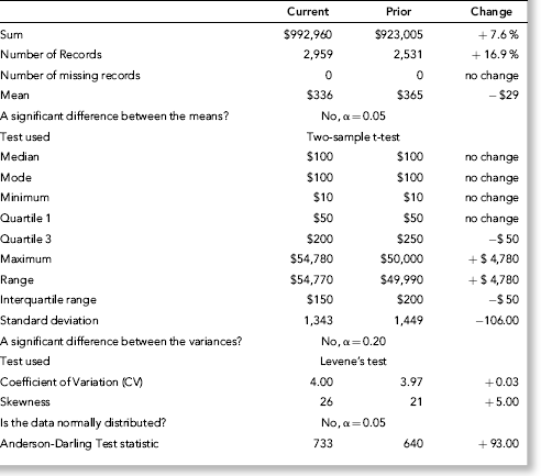
The first set of descriptive statistics in the parallel scan (see Table 9.1) give us an overview of the data, much like the data profile gives us an overview in the Nigrini Cycle. The overview consists of the sum, the number of records, and the number of missing records. In a forensic analytic project the sum should agree with, or should be reconcilable with the trial balance to ensure that all the account details are included in the analysis. Missing records might indicate fraud, or processing or internal control issues.
Table 9.1 The Descriptive Statistics of Alumni Gifts for Two Consecutive Years.
The second set of descriptive statistics relates to measures of central tendency. The mean, median, and the mode are often used in the financial press and are understood by most forensic investigators. A large change in either of these values should be investigated. The difference between two means can be formally tested using the two-sample t-test. The auditing concept of materiality and statistical significance are not the same, and a significant difference should not be seen to be a material difference. In Chapter 6 we saw that with large data sets even small differences between the actual and expected proportion give us statistically significant differences due to the excess power problem. We will have to carefully interpret the results of our descriptive statistics.
The third set of descriptive statistics measures the variability or the spread of the numbers. This includes the minimum and maximum, the interquartile range, and the range (the maximum minus the minimum amount). The interquartile range measures the spread in the middle 50 percent of the data and is the difference between the 75th percentile and the 25th percentile. The range is the difference between the 100th percentile and the minimum. This set of values includes the minimum amount that might yield investigative insights if the number was negative in a data set that should not contain negative numbers (e.g., wages, inventory counts, coupon or rebate amounts, or odometer readings). The variability measures also include the standard deviation that measures the average deviation about the mean. Large changes in the variability values could be a red flag for fraud or error. There could be changes in variability even though the measures of central tendency are largely unchanged. The difference between the standard deviations can be formally tested by testing the difference between the variances using Levene's test. To assess whether the standard deviation is big or small we use the coefficient of variation (CV), which gives us the standard deviation as a percentage of the mean. This is a useful measure because it allows us to interpret the standard deviation in the context of the mean.
The final set relates to the shape of the distribution of the data. The first such measure is skewness, which tells us whether the numbers are evenly distributed around the mean. Data that is positively skewed consists of many small amounts and fewer large amounts. This is usually the pattern found in the dollar amounts of invoices paid (expenses) or sales invoices (sales). Most financial data are positively skewed because we usually have many small numbers and only a few large numbers. In contrast, data with a negative skewness measure has many large numbers and fewer smaller numbers. These cases are relatively rare. Another shape measure is the Anderson-Darling test statistic that measures the closeness of fit to the normal distribution. A calculated test statistic of 0.80 would signal that the data is normally distributed. Financial data seldom conform to the normal distribution except possibly for salaries or wages data. The Anderson-Darling statistic can be used to test that the departure from normality is approximately the same from period to period. More information on the statistical terms and tests in this section can be found in the NIST/SEMATECH e-Handbook of Statistical Methods at www.itl.nist.gov/div898/handbook.
The first graphical method of describing data is the histogram. Newbold, Carlson, and Thorne (2010) describe a histogram as a graph consisting of vertical bars constructed on a horizontal line that is marked off with intervals. These intervals should be inclusive and should not overlap. Each record should belong to one and only one interval. The height of each bar in the histogram is proportional to the number of records in the interval. Chapter 4 discusses histograms and also how the histogram values can be calculated in Access and graphed in Excel.
The number of intervals used in a histogram is at the discretion of the forensic investigator. Newbold, Carlson, and Thorne (2010) suggest 14–20 intervals if there are more than 5,000 records. This will give a very crowded histogram especially when current and prior year histograms are being compared side by side. In forensic analytics it seems that 10 intervals would work well. Each interval should have a neat round number as the upper bound (e.g., $50, $100, $150) and should preferably contain enough records so that at least a small bar is visible for every interval. No real insights are obtained from a histogram that has one or two intervals containing most of the records. The final (10th) interval should be for all amounts greater than the prior upper bound (for example, $450 and higher). This makes the final interval width much wider than those of the first nine intervals and this interval should therefore be clearly labeled.
The second graphical method of describing data is through an adaptation of Benford's Law, which we will call My Law. The My Law concept was developed when an airline changed its pilot payroll systems. The logic in using the test was that the digits and number patterns from the new system should be the same (or at least similar) to those from the old system since nothing had changed except the processing system.
The case study involves alumni gifts to a college. Alumni gifts are an important and significant source of revenue for most higher education institutions. The funds are used to support student services, academic programs, athletics, and other extracurricular activities. The college in this case is a liberal arts college that draws its students from the surrounding region. Each gift amount was a contribution from a past student. The contributions are for two consecutive years. The numerical descriptive statistics for the parallel scan are shown in Table 9.1.
Table 9.1 shows the numerical descriptive statistics of the gift data. The statistics give an overview of the data, show measures of central tendency and variability, and describe the shape of the distribution. In the current year the college received a total of $992,960, which was an increase of 7.6 percent over the prior year. In dollar terms the increase amounted to about $70,000. In the current year they received 2,959 gifts from past students, which was a 17 percent increase over the prior year. The increase in the total dollars was because of an increased number of phone calls and letters asking for donations. The data contained no null (missing) amounts.
With respect to central tendency, the mean decreased from $365 to $336. The decrease in the mean agrees with the fact that the percentage increase in the number of gifts was greater than the percentage increase in the total dollars. The decrease in the average gift amount might signal that funds are being misappropriated. The review revealed that there was a special effort to get more donations and past students were encouraged to make a gift even if it was small. Once someone made some contribution, there was a good chance of a bigger gift next time. The two-sample t-test was used for a comparison of the means and the difference between the means was not found to be significant. The mean was greater than the median of $100 indicating that the data was positively skewed. In both periods the minimum, maximum, and the range are comparable and no red flag is raised from an investigation perspective. Both the quartile 3 amount and the interquartile range differ by $50. The effort to get more gifts, even if they were small, also explained the decrease in the quartile 3 amount and the interquartile range. The mode (the most frequently occurring amount) was unchanged at $100 for both periods.
The measures of variability show that the standard deviation was largely unchanged. The standard deviation paints a more complete picture of dispersion than does the range. Two data tables may have the same range, but the amounts in one may be concentrated near the center of the range and in the other they may be concentrated in the tails of the distribution. Levene's test for the difference between the variances gave a test statistic of 0.31, which translates to a p-value of 0.577. This means that the difference between the variances is not significant. Experience with Levene's test has shown that the difference between the variances must be quite large before the test indicates a significant difference even at a significance level of 0.20. The coefficient of variation is little changed. The standard deviations are quite large when compared to the means in each period indicating that there is a large spread compared to the average values. The variability measures show no major change from period to period.
The shape measures show that the skewness measure increased from 21 to 26. This was also because of the additional small ($10 to $50) gifts. The Anderson-Darling test was used to assess conformity to the familiar bell-shaped Gaussian distribution. With the large skewness measures, a close fit to the normal curve is unlikely because the normal distribution is symmetric. The Anderson-Darling test statistics of 733 and 640 indicate large departures from normality (the bell-shaped curve) but the extent of the departure from normality is approximately equal.
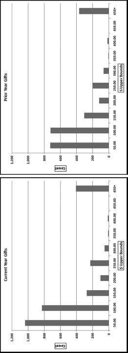
The histograms of the gift amounts are shown in Figure 9.1. Using 10 intervals and a width of $50 for each interval gives a final 10th interval for amounts of $450 and higher. The y-axis (the count) for the current and prior year should be comparably calibrated (from 0 to 1,200 in this case) so that the histograms can be compared visually. For the gift data the histograms are similar except for the first two intervals (0 to $50, and $50.01 to $100), which have noticeably higher counts in the current period. The explanation for this difference was the increased effort to get more gifts in the current year (however small they might be).
Figure 9.1 The Histograms of the Current and Prior Year Gift Amounts
The gift amounts were not expected to follow Benford's Law because gifts are influenced by human thought since the donor thinks of an amount to give. This number invention process usually sees a gravitation toward round numbers that are psychological thresholds. Also, donor recognition levels also influence the gift amounts. The first-order results for both years are shown in Figure 9.2.
Figure 9.2 The Results of the First-Order Tests of the Gift Data
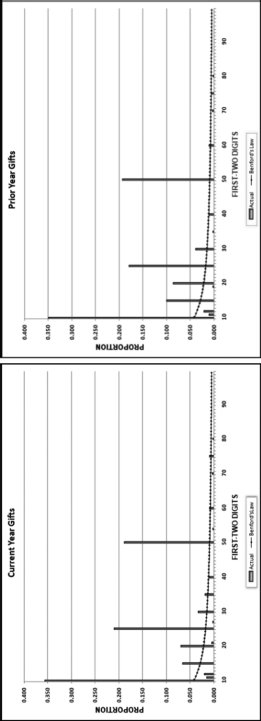
Chapter 6 discussed assessing conformity to Benford's Law and the list of possible conformity tests included the chi-square and K-S tests, the Mean Absolute Deviation (MAD), and the mantissa arc test. The tests were geared toward assessing conformity to Benford's Law. In this case the goal is to compare the current and prior data. The prior period's first-order graph takes the place of Benford's Law. In the first application of this concept, the prior period data was called My Law. A large difference between the current data and My Law indicates that something has changed and the change could be due to errors or fraud, or a change in circumstances.
The MAD as shown in Equation 6.4 is the suggested statistic for measuring conformity. In this application the MAD is calculated in the same way except that the EP (Expected Proportion) is now the prior data. An extract from the table with the MAD calculation is shown in Figure 9.3.
Figure 9.3 An Extract from the Worksheet Calculating the MAD
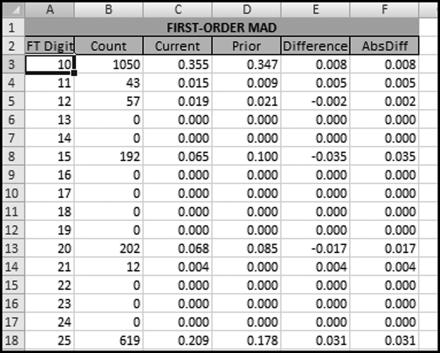
The MAD for the current and the prior period data is 0.0015. The guidelines for assessing conformity in a My Law application are set out in Table 9.2.
Table 9.2 The Mean Absolute Deviation Cutoff Values for a My Law Application.
| MAD range | Conclusion |
| 0.0000 to 0.0024 | Close conformity |
| 0.0024 to 0.0036 | Acceptable conformity |
| 0.0036 to 0.0044 | Marginally acceptable conformity |
| Above 0.0044 | Nonconformity |
Table 9.2 sets out ranges for the My Law application that are twice as wide as those for the usual first-order test. The prior distribution is not as stable as that of Benford's Law. There is some room for error and some judgment is used. The forensic investigator will need to evaluate whether the immediately prior period is the best benchmark. Another possible benchmark would be to look at two or three prior periods and then to average the results. Given the instability of the prior distribution we should allow for larger differences before we reach a nonconformity conclusion. The MAD for the gift data is 0.0015 and this gives us a comfortable close conformity conclusion.
The numerical and graphical descriptive statistics of the parallel scan show that the current data detail is reasonably similar to the prior data detail. The overview measures, together with the statistics relating to central tendency, variability, and the shape of the distribution show that the detail is consistent from year to year. The drive for additional gifts (however small) explains all of the main time-related differences. The histogram and the digit patterns show a consistency from year to year, except for some differences due to the drive for additional gifts. These results suggest a reduced risk of errors or fraud.
An Analysis of Fraudulent Data
The current data was seeded with fraud. The realistic, but hypothetical, fraud is based on the recognition that donors receive from the college based on the amount of the gift. Donor names and recognition levels are listed in various college publications, and formal events are held for members of various recognition levels. It is normal for donors to give an amount that would just qualify for some recognition level. The fraud in this case was that the accountant diverted funds for his personal use, constrained by the fact that the donor would complain if they were given an inferior recognition level at college events. With the recognition level constraint only about one-half of the gifts had any dollars that could be “skimmed off the top.” An example of the fraud is recording $7,000 as $5,000 to siphon off $2,000 leaving the donor still a member of the “Platinum Society,” which recognizes gifts from $5,000 to $9,999. There was no skimming (theft) of amounts under $150 because the theft of such small amounts was not worth the risk. This $150 lower limit meant that only about 16 percent of the gift amounts were subject to skimming. The largest gift was reduced by $40,000 to $14,780 since the accountant would still want an odd number here and there to account for gifts of appreciated stock. The fraudulent data is therefore the table of old current data with each “skimable number” over $150 reduced to the lower threshold for its recognition level. The number of records is unchanged, but one-sixth of the gift amounts have been reduced and the rest are unchanged from the data analyzed in Table 9.3.
Table 9.3 The Descriptive Statistics of the Fraudulent Data.
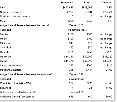
Table 9.3 shows the descriptive statistics of alumni gifts for the current fraudulent year and the prior year together with the change for the year. The abbreviation α refers to the significance level of the test.
The descriptive statistics of the fraudulent data and the prior data are shown in Table 9.3. The overview shows that the number of records has increased and the explanation of the increased drive for gifts of any size is an acceptable explanation for the higher count. The sum shows a decrease and this should raise a red flag from a fraud perspective because the college made a concerted effort to raise more gift dollars than the prior year. The change in the sum is consistent with the presence of fraud (or error).
The central tendency statistics show that the mean decreased by $75. This change is consistent with the presence of fraud. The difference between the means is now statistically significant at the 0.05 level and can therefore not be attributed to random fluctuations. The total amount skimmed from the gifts was $135,000 and this loss was large enough to cause a significant difference between the means. Table 9.3 also shows that the quartile 3 value of $125 and the maximum value of $14,780 are both much less than the comparable numbers for the prior period.
The variability statistics show that the standard deviation decreased from about 1,450 to 750. The fraudulent data had far less dispersion (spread) about the mean. This reduction in variability was directly because of the fraud. The accountant siphoned off large amounts from the large gifts (above $10,000) in that they had almost all of their excesses (the amount needed to be in the top gift tier) diverted. The large reductions in the large amounts caused the standard deviation to decrease. The decrease was large enough to cause a significant difference between the variances using Levene's test. This test requires a reasonably dramatic difference to be significantly different and past experience suggests using a significance level of 0.20 for this test. The fraud caused the standard deviation to halve and so the CV was also notably reduced by about one-third. The reductions in skewness, standard deviation, and CV, all indicate large decreases in dispersion. The decrease in dispersion is evident from the decrease in the range. The variability measures indicate that the account detail has changed.
The skewness measure decreased from 21 to 7. The amounts siphoned off from the large gifts made the distribution more symmetric. The skewness measure can be highly influenced by just a few large amounts. The Anderson-Darling statistic is virtually unchanged and it is therefore not overly influenced by a small group of large numbers. The skewness measure correctly indicates that the shape of the distribution has changed.
The statistical overview and measures of central tendency can be calculated with Excel. The data analysis functions are found using Data→Analysis→Data Analysis→Descriptive Statistics. The descriptive statistics of the fraud data is shown in Figure 9.4.
Figure 9.4 Descriptive Statistics Produced by Excel
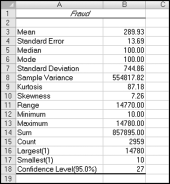
The descriptive statistics are shown in Figure 9.4. The Excel results should be formatted to zero or two decimals where appropriate. The quartile 1 and quartile 3 values can be calculated in Excel using the Large function. Excel's output includes the standard deviation and the skewness measure. Access can compute some of the descriptive statistics but Access is limited in what it can do in this arena. For example, calculating the median is possible in Access but it does require some reasonably nimble Access gymnastics.
Minitab does an excellent job with descriptive statistics. This software package is developed by the Pennsylvania State University. A free trial version can be downloaded from the Minitab website. The Minitab steps to calculate the descriptive statistics are Stat→Basic Statistics→Display Descriptive Statistics. The fraud data results are shown in Figure 9.5.
Figure 9.5 A Minitab Dialog Screen and the Descriptive Statistics
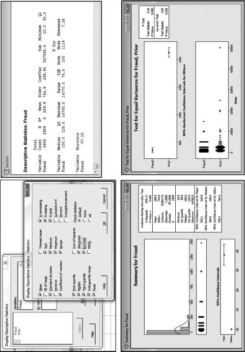
The Minitab results are shown in Figure 9.5. The Anderson-Darling test is run in Minitab using Stat→Basic Statistics→Graphical Summary and the comprehensive results are shown in the third panel in Figure 9.5. Levene's test for equal variances is run using Stat→Basic Statistics→2 Variances. Minitab is user-friendly, and easy to use and to understand. Data can be imported into Minitab using the familiar Copy and Paste steps. Extensive help is available in Minitab to explain the results and the formulas used in the program. Minitab is the preferred tool for the calculation of descriptive statistics.
The histograms of the fraudulent and the prior data are shown in Figure 9.6. The results show that the counts for the lower values for the fraudulent data are higher than the counts for the lower values in the original data.
Figure 9.6 The Histograms of the Gift Amounts
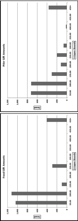
The increased drive for gifts of any size is a plausible explanation for the higher counts in the $50 and $100 intervals in the fraud data. The histogram gives us no indication that the sum has decreased by 14 percent because histograms measure counts and not sums. Most of the siphoning off by dollar value took place in the bin for $450+, and while the dollar amounts were reduced (in one case by $40,000 and in another case by $17,895), the counts (which is what a histogram is all about) were not noticeably affected. This reminds us that each descriptive statistic or graph only looks at one characteristic of the data. The fraud histogram shows that the fraud data has counts of zero for the $200, $300, $350, $400, and $450 intervals whereas most of these intervals had small bars (positive counts) in the prior year. The newly empty intervals are quite suspicious and correctly signal a change in the data detail. The next test is a comparison of the first-order tests in Figure 9.7.
Figure 9.7 The Results of the First-Order Tests
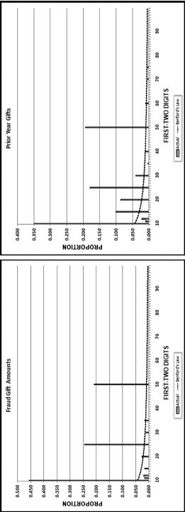
The first-order tests in Figure 9.7 show a surprising result. The focus is on a comparison of the first-order results between the current and the prior year, with the Benford proportions included only as reference points. The digit patterns of the fraudulent data and the prior data are not too different. The y-axes are calibrated equally from 0 to 0.50 so that the differences are easier to see. The MAD of 0.00451 signals nonconformity or that there is a large difference between the two years. The fact that the distributions are not wildly different is somewhat surprising. This could be because there were only 470 skims (about 16 percent of the amounts) and in some cases the skims did not affect the first digit (e.g., amounts in the $150 to $199 range were reduced to $100) or the changes might have cancelled each other. These results themselves are a bit anomalous in that we have a nonconformity conclusion using the MAD even though the fraud only affected a small percentage of the detail in the data table.
The second-order test of Benford's Law was not performed on the data because the data was not drawn from a continuous distribution with a smooth density function as is a requirement of this test. The type of data (alumni gifts) was such that there were unused intervals of numbers that were entirely missing from the data set, followed by clusters of numbers at certain favored gift amounts. The data sets contained about 3,000 records each but there were too few different numbers being used to get any useful pattern from the second-order test.
The last-two digits, the summation test, and the number duplication tests are not seen to be very useful in a comparison of current data and prior period data. The suite of current and prior data tests only includes descriptive statistics, histograms, and the first-order test.
The forensic analytic tests in the chapter relate to a comparison of the transaction details of the current period to the transaction details of the prior period. These tests would help to assess the risk of fraud or errors. The tests are made up of numerical statistics related to a data overview, and measures of central tendency, variability, and the shape of the distribution. The tests also include two graphical methods related to the shape of the distribution and the first-order test.
The case study dealt with gift amounts given to a college over a period of two consecutive years. The descriptive statistics and the graphical methods showed that there were differences between the two data sets. The explanation for the differences was that the college embarked on a special drive to get more people to donate, even if the gift amounts were small. In the second analysis the current year gift data was seeded with a fraud where the accountant siphoned off dollar amounts from about one-sixth of the gifts. The new fraud descriptive statistics showed some substantial differences between the fraudulent data and the gifts from the prior year. The numerical descriptive statistics signaled a change in the details. For the graphical methods, the histogram signaled that the detail had changed. The first-order test also signaled a noticeable change in the account detail. The current set of digit patterns were compared to the digit patterns for the prior year and this application was called My Law. In some cases the changes were evident from some tests and in other cases the fraud or errors were evident from other tests. Even in the absence of errors or fraud, the analysis of the detail gives insights into the entity and its environment that might prove to be useful in a forensic investigations environment.
Discussions with external auditors indicated that most practicing auditors would understand the overview statistics and some of the central tendency measures. The use of the other numerical and graphical methods would have to be preceded by some training on understanding and interpreting these statistics. Auditors and forensic investigators would have to understand that some numeric and graphical values will have small changes from period to period due to normal changes in conditions that are unrelated to fraud or error. Forensic users will have to identify what makes up a substantial change and one worthy of further investigation. The “investigate further” decision is similar to what auditors already do with the familiar profitability and liquidity ratios.
Auditors also indicated that they are keen to show that their audit provides some value above and beyond the audit report. These value-added discussions usually take place after the audit in the management letter meeting with the audit committee. The results of an analysis using these descriptive statistics, with some anomalous results detected, would be something that they could use at these post-audit meetings. These tests could even be suggested to management as tests that they (management) could perform on an ongoing basis on their data. The auditors would then use the results in the audit as evidence of the monitoring of controls.
