
Chapter 5
Benford's Law
The Basics
The Benford's Law–based tests signal abnormal duplications. The mathematics of Benford's Law gives us the expected or the normal duplications, and duplications above the norm are abnormal or excessive. Bolton and Hand (2002) state that the statistical tools for fraud detection all have a common theme in that observed values are usually compared to a set of expected values. They also say that depending on the context, these expected values can be derived in various ways and could vary on a continuum from single numerical or graphical summaries all the way to complex multivariate behavior profiles. They contrast supervised methods of fraud detection that use samples of both fraudulent and nonfraudulent records, or unsupervised methods that identify transactions or customers that are most dissimilar to some norm (i.e., outliers). They are correct when they say that we can seldom be certain by statistical analysis alone that a fraud has been perpetrated. The forensic analysis should give us an alert that a record is anomalous, or more likely to be fraudulent than others, so that it can be investigated in more detail. The authors suggest the concept of a suspicion score where higher scores are correlated with records that are more unusual or more like previous fraudulent values. Suspicion scores could be computed for each record in a table and it would be most cost-effective to concentrate on the records with the highest scores. Their overview of detection tools includes a review of Benford's Law and its expected digit patterns. Chapters 15 and 16 show how formal risk scores (like their suspicion scores) can be developed from predictors for the forensic units of interest.
Benford's Law gives the expected frequencies of the digits in tabulated data. As a fraud investigation technique Benford's Law also qualifies as a high-level overview. Nonconformity to Benford's Law is an indicator of an increased risk of fraud or error. Nonconformity does not signal fraud or error with certainty. Further work is always needed. The next four chapters add ever-increasing layers of complexity. The general goal, though, is to find abnormal duplications in data sets. The path from Chapter 4 to Chapter 12 is one that starts with high-level overview tests and then drills deeper and deeper searching for abnormal duplications of digits, digit combinations, specific numbers, and exact or near-duplicate records. Benford's Law provides a solid theoretical start for determining what is normal and what constitutes an abnormal duplication. The cycle of tests is designed to point the investigator toward (a) finding fraud (where the fraudster has excessively duplicated their actions), (b) finding errors (where the error is systematic), (c) finding outliers, (d) finding biases (perhaps where employees have many purchases just below their authorization level), and (e) finding processing inefficiencies (e.g., numerous small invoices from certain vendors).
The format of this chapter is to review Benford's original paper. Thereafter, the Benford's Law literature is reviewed. The chapter then demonstrates the standard set of Benford's Law tests. These tests concentrate only on a single field of numbers. The chapter continues with the invoices data from the previous chapter. The tests are demonstrated using a combination of Access and Excel.
Benford's Law gives the expected frequencies of the digits in tabulated data. The set of expected digit frequencies is named after Frank Benford, a physicist who published the seminal paper on the topic (Benford, 1938). In his paper he found that contrary to intuition, the digits in tabulated data are not all equally likely and have a biased skewness in favor of the lower digits.
Benford begins his paper by noting that the first few pages of a book of common logarithms show more wear than the last few pages. From this he concludes that the first few pages are used more often than the last few pages. The first few pages of logarithm books give us the logs of numbers with low first digits (e.g., 1, 2, and 3). He hypothesized that the worn first pages was because most of the “used” numbers in the world had a low first digit. The first digit is the leftmost digit in a number and, for example, the first digit of 110,364 is a 1. Zero is inadmissible as a first digit and there are nine possible first digits (1, 2, . . ., 9). The signs of negative numbers are ignored and so the first-two digits of −34.83 are 34.
Benford analyzed the first digits of 20 lists of numbers with a total of 20,229 records. He made an effort to collect data from as many sources as possible and to include a variety of different types of data sets. His data varied from random numbers having no relationship to each other, such as the numbers from the front pages of newspapers and all the numbers in an issue of Reader's Digest, to formal mathematical tabulations such as mathematical tables and scientific constants. Other data sets included the drainage areas of rivers, population numbers, American League statistics, and street numbers from an issue of American Men of Science. Benford analyzed either the entire data set at hand, or in the case of large data sets, he worked to the point that he was assured that he had a fair average. All of his work and calculations were done by hand and the work was probably quite time-consuming. The shortest list (atomic weights) in his list had 91 records and the largest list had 5,000 records.
Benford's results showed that on average 30.6 percent of the numbers had a first digit 1, and 18.5 percent of the numbers had a first digit 2. This means that 49.1 percent of his records had a first digit that was either a 1 or a 2. At the other end of the “digit-scale” only 4.7 percent of his records had a first digit 9. Benford then saw a pattern to his results. The actual proportion for the first digit 1 was almost equal to the common logarithm of 2 (or 2/1), and the actual proportion for the first digit 2 was almost equal to the common logarithm of 3/2. This logarithmic pattern continued through to the 9 with the proportion for the first digit 9 approximating the common logarithm of 10/9.
Benford then derived the expected frequencies of the digits in lists of numbers and these frequencies have now become known as Benford's Law. The formulas for the digit frequencies are shown below with D1 representing the first digit, D2 the second digit, and D1D2 the first-two digits of a number:

where P indicates the probability of observing the event in parentheses and log refers to the log to the base 10. The formula for the expected first-two digit proportions is shown in Equation (5.3). For the first-two digits, the expected frequencies are also highly skewed, and range from 4.139 percent for the 10 combination down to 0.436 percent for the 99 combination. The first-two digits of 110,364 are 11. Using Equation (5.3), the expected proportion for the first-two digits 64 would be calculated as follows:

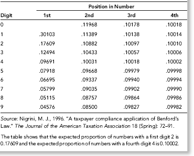
The expected frequencies for the digits in the first, second, third, and fourth positions is shown in Table 5.1. As we move to the right the digits tend toward being equally distributed. If we are dealing with numbers with three or more digits then for all practical purposes the ending digits (the rightmost digits) are expected to be evenly (uniformly) distributed.
Table 5.1 The Expected Digit Frequencies of Benford's Law.
In the discussion section of his paper Benford noted that the observed probabilities were more closely related to “events” than to the number system itself. He noted that some of the best fits to the logarithmic pattern (of the digits) was for data in which the numbers had no relationship to each other, such as the numbers from newspaper articles. He then associated the logarithmic pattern of the digits with a geometric progression (or geometric sequence) by noting that in natural events and in events of which man considers himself the originator there are plenty of examples of geometric or logarithmic progressions. Benford concluded that nature counts e0, ex, e2x, e3x, and so on, and builds and functions accordingly because numbers that follow such a pattern end up with digit patterns close to those in Table 5.1. Figure 5.1 is an example of a geometric sequence of 1,000 numbers ranging from 10 to 100.
Figure 5.1 A Geometric Sequence of 1,000 Records with the Numeric Amounts Ranging from 10 to 100
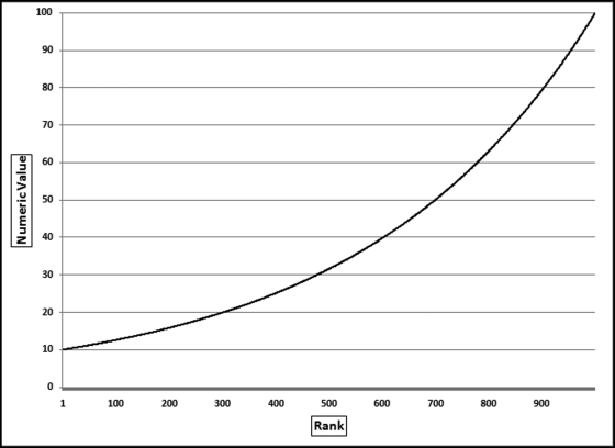
A geometric sequence such as is shown in Figure 5.1 is a sequence of terms in which each successive term is the previous term multiplied by a common ratio. The usual mathematical representation for such a sequence is given by

where a is the first term in the sequence, r is the common ratio, and n denotes the nth term. In Figure 5.1, a equals 10, and r (the common ratio) equals 1.002305. There are 1,000 terms in the sequence shown in Figure 5.1. Using the assumption that the ordered (ranked from smallest to largest) records in a data set is made up of natural numbers from a geometric sequence, Benford then derived the expected frequencies of the digits for tabulated “natural” data. The formulas are shown in Equations 5.1, 5.2, and 5.3 and the first through fourth digit frequencies are shown in Table 5.1.
Benford provided no guidance as to when a data set should follow the expected frequencies other than a reference to natural events and science-related phenomena developed by people. Benford gave examples of geometric progressions such as our sense of brightness and loudness. He also referred to the music scales, the response of the body to medicine, standard sizes in mechanical tools, and the geometric brightness scale used by astronomers. The strong geometric foundation of Benford's Law means that a data table will have Benford-like properties if the ranked (ordered from smallest to largest) records closely approximate a geometric sequence. Chapter 8 goes further with the discussion of the geometric basis of Benford's Law.
From Theory to Application in 60 Years
The first Benford's Law papers were published by Goudsmit and Furry (1944) and Furry and Hurwitz (1945). The 1944 paper suggests that Benford's Law is merely the result of the way that we write numbers and the 1945 paper is a mathematical discussion of Benford's formulas. Interestingly, Stigler (1945) wrote an unpublished working paper in which he challenged the basis of Benford's Law and gave an alternative distribution of the digits in lists of numbers. This was later called Stigler's Law. Nobel-laureate Stigler never published the paper. Stigler's logic is questioned in Raimi (1976) and it would therefore appear that to win a Nobel Prize, one should know what to publish and what to leave in working paper format.
The third Benford's Law paper was published in 1948 in The Journal of General Psychology (Hsu, 1948). Hsu apparently saw the link between Benford's results and human behavior. Hsu's only reference in his 1948 paper is to Benford's 1938 paper. Hsu had 1,044 faculty and students invent a four-digit number with the requirement that the number was original and should not represent an event, a fact, or a date. His results showed that the numbers did not follow Benford's Law and he believed that this was because Benford's Law did not apply to mental numbers. These results are an important early finding and shows that nonconformity to Benford's Law is not always an indicator of fraud or error.
The most significant advance in the 1960s was by Pinkham (1961). Pinkham posed the question that if there were indeed some law governing digital distributions then this law should be scale invariant. That is, if the digits of the areas of the world's islands, or the length of the world's rivers followed a law of some sort, then it should be immaterial if these measurements were expressed in (square) miles or (square) kilometers. Pinkham then proved that Benford's Law is scale invariant under multiplication. So, if all the numbers in a data table that followed Benford's Law were multiplied by a (nonzero) constant, then the new data table would also follow Benford's Law. A list of numbers that conform to Benford's Law is known as a Benford Set. What is notable is that Pinkham proved that it was only the frequencies of Benford's Law that were invariant under multiplication. So if a data set has digit frequencies other than those of Benford's Law, then multiplication by a (nonzero) constant will result in changed digital frequencies. It would seem logical that the closer the fit before multiplication (irrespective of the constant), then the closer the fit after multiplication. It is interesting that Pinkham's introduction states that any reader formerly unaware of Benford's Law would find an actual sampling experiment “wondrously tantalizing.” Fifty years ago such an experiment would have required a great deal of effort. It is only now that such an experiment would really be wondrously tantalizing without being mentally exhausting.
Good (1965) was the first person to formally use Benford's Law. Good noted that certain random number tables had been formed by taking the middle three digits of the areas of English parishes. Good claimed that this would not produce random number tables because under Benford's Law the digits are not all equally likely, and such a table would have random numbers slightly biased toward the low digits.
There were two Benford developments in 1966. Feller (1966) developed an alternative proof for Benford's Law and Flehinger (1966) also developed an alternative proof for Benford's Law. Flehinger's proof has been criticized because she uses a special summation and averaging method (Holder sums), and mathematicians contend that using special tricks that end up with Benford's frequencies do not constitute a proof. That is, if the end result of your mathematical calculations equals Benford's Law, it does not mean that you have proved Benford's Law.
The first Asian contribution to the field came from the Indian Statistical Institute by way of Adhikari and Sarkar (1968) who developed a few theorems relating to numbers distributed uniformly over the range 0 to 1. They showed that after certain mathematical operations the numbers formed a Benford Set. In the next year Raimi (1969a) provided mathematical support for Benford's Law using Banach and other scale invariant measures. Raimi (1969b) is an excellent nonmathematical review of Benford's Law with some intuitive explanations of what later came to be called the first digit phenomenon in many papers. The second Raimi paper was the first time that Benford's Law made it into a widely circulated and highly respected medium (Scientific American). There was more to 1969 than the Woodstock rock festival because Adhikari (1969), now on a roll, followed his earlier paper with a few more theorems. Knuth (1969) completed the 1960s with a simplified proof of Flehinger's result and a reasonably in-depth discussion of Benford's Law.
The 1970s started with Hamming (1970) and an application of Benford's Law. Hamming considers the mantissa distribution of products and sums and gives applications of Benford's Law in round-off error analysis and computing accuracy considerations. The early 1970s also started a stream of articles by Fibonacci theorists who showed that the familiar Fibonacci sequence (1, 1, 2, 3, 5, 8, . . .) follows Benford's Law perfectly. The Fibonacci Quarterly journal became the first journal to publish six Benford's Law papers in the same decade. It is interesting that the Fibonacci sequence plays a role in The Da Vinci Code, the best-selling novel by Dan Brown. The Fibonacci sequence has also been featured in popular culture including cinema, television, comic strips, literature, music, and the visual arts. To see a reasonably good fit to Benford's Law the sequence should have about 300 or more elements. The more Fibonacci elements there are, the closer is the fit to Benford's Law. In the first of these papers Wlodarski (1971) shows that the first digits of the first 100 Fibonacci and the first 100 Lucas numbers approximates the expected frequencies of Benford's Law. Sentence (1973) tests the first 1,000 Fibonacci and Lucas numbers showing a close fit to Benford's Law. Several years later Brady (1978) tests the first 2,000 Fibonacci and Lucas numbers with an even closer fit to Benford's Law. Technically speaking, the Fibonacci sequence is an example of an asymptotically (approximate) geometric sequence with r (the common ratio) tending toward (1 + √5)/2. These 1970s studies would have used reasonably complex computer programming because the Fibonacci numbers become very large very quickly and by the 100th Fibonacci number Excel has started to round the number to 16 digits.
By now researchers had begun to question whether Benford's Law had practical purposes and Varian (1972) questioned whether Benford's Law could be used to assess the reliability of forecasts. He tabulated the first-digit frequencies of a few sets of demographic data. The original data conformed quite closely to Benford's Law. He then checked the frequencies of forecasts made from the data. The forecasts also followed Benford's Law. Varian concluded that checking forecasts against Benford's Law was a potential test of the reasonableness of the forecasts. Another paper addressing the usefulness of Benford's Law appeared just two years later when Tsao (1974) applied Benford's Law to round off errors of computers.
Goudsmit (1977) delved into the Benford's Law past and shared the insight that the paper following Benford's paper in the journal was an important physics paper by Bethe and Rose. Physicists that read the Bethe and Rose paper saw the last page of Benford's paper on the left-hand page in the journal. They presumably found it interesting and went back to read all of Benford's paper. Goudsmit should know because he coauthored the first paper on the topic. It is amazing to think that had a stream of literature not been started by the readers of Bethe and Rose, that Benford's gem would not have been noted by academics or practitioners. It would seem that even if forensic analytic practitioners noted casually that more numbers began with a 1 than any other digit, they would probably not think that a precise expected distribution existed.
The most influential paper of the 1970s was Ralph Raimi's 1976 review paper published in American Mathematical Monthly. Raimi (1976) reviews the literature, which at that time came to 37 papers, including the original paper by Benford. Raimi also lists 15 other papers that mentioned Benford's Law in passing. According to Google Scholar, Raimi's 1976 paper has been cited by 160 Benford papers. Raimi starts with the digit frequency results from just a few data sets reinforcing the belief that data analysis prior to the 1990s was a labor-intensive process. Raimi includes an interesting result related to electricity usage. Raimi then continues with what he calls “a bit of philosophy.” He then critiques some approaches to proving Benford's Law by noting that just because some mathematical method gives the Benford probabilities as their result, this does not prove Benford's Law. This is because there are many methods that will not result in the Benford probabilities. Raimi's concluding comments include a few gems such as the fact that he liked Varian's suggestion that Benford's Law could be used as a test of the validity of scientific data, and his belief that “social scientists need all the tools of suspicion they can find” (Raimi, 1976, 536).
The 1980s
The 1980s began with two Benford papers that addressed the potential usefulness of Benford's Law. Becker (1982) compared the digit frequencies of failure rate and Mean-Time-to-Failure tables with Benford's Law. He concluded that Benford's Law can be used to “quickly check lists of failure rate or MTTF-values for systematic errors.” Nelson (1984) discussed accuracy loss due to rounding to two significant digits. He used Benford's Law to compute the average maximum loss in accuracy.
The Benford's Law literature has included some research that questions the validity of Benford's Law. Some questions should be expected, given the counterintuitiveness of the digit patterns. What is surprising in this case is the source of the challenge, namely Samuel Goudsmit (who published the first Benford's Law paper in 1944). Raimi (1985) discusses the basis and logic of Benford's Law and his 1985 paper concludes with an extract from a letter from Samuel Goudsmit (dated 21 July, 1978) in which Goudsmit claims that:
To a physicist Simon Newcomb's explanation of the first-digit phenomenon is more than sufficient “for all practical purposes.” Of course here the expression “for all practical purposes” has no meaning. There are no practical purposes, unless you consider betting for money on first digit frequencies with gullible colleagues a practical use. (Goudsmit as quoted in Raimi, 1985, 218)
Tax evasion, auditing, and forensic analytics research shows that there are practical uses of Benford's Law. It is interesting that Goudsmit published the first paper on Benford's Law after the publication of Benford's paper (Goudsmit and Furry, December, 1944), and Ian Stewart wrote a paper on Benford's Law that starts with a story about a trickster betting on first digits with the public at a trade fair in England (Stewart, 1993).
The 1980s also saw the first accounting application by Carslaw (1988). He hypothesized that when company net incomes are just below psychological boundaries, accountants would tend to round these numbers up. For example, numbers such as $798,000 and $19.97 million would be rounded up to numbers just above $800,000 and $20 million respectively. His belief was that the latter numbers convey a larger measure of size despite the fact that in percentage terms they are just marginally higher. Management usually has an incentive to report higher income numbers. Evidence supporting such rounding-up behavior would be an excess of second digit 0s and a shortage of second digit 9s. Carslaw used the expected second-digit frequencies of Benford's Law and his results based on reported net incomes of New Zealand companies showed that there were indeed more second digit 0s and fewer second digit 9s than expected.
Hill (1988) was the second Benford-based experimental paper after Hsu (1948). He provided experimental evidence that when individuals invent numbers these numbers do not conform to Benford's Law. Hill's 742 subjects had no incentive to bias their six-digit numbers upward or downward. Hill used the Chi-square and Kolmogorov-Smirnoff tests plus a little creativity to evaluate his results. His results showed that the first and second digits were closer to being uniformly distributed than being distributed according to Benford's Law. It is interesting that two subjects invented a six-digit string of zeroes (these results were discarded). Number invention has received much subsequent attention with results showing that autistic subjects were more likely to repeat digits (Williams, Moss, Bradshaw, and Rinehart, 2002). The papers on this topic include Mosimann, Wiseman, and Edelman (1995) who show that even with a conscious effort, most people cannot generate random numbers. Interestingly their results showed that 1, 2, and 3 were the most favored digits in number invention situations.
Carslaw's paper was soon followed by Thomas (1989). Thomas found excess second-digit zeros in U.S. net income data. Interestingly, Thomas also found that earnings per share numbers in the United States were multiples of 5 cents more often than expected. In a follow-on study Nigrini (2005) showed that this rounding-up behavior seems to have persisted through time. Quarterly net income data from U.S. companies showed an excess of second-digit zeroes and a shortage of second-digit 8s and 9s for both first quarters in 2001 and 2002. The second-digit zero proportion was slightly higher in 2002. This result was surprising given that this period was characterized by the Enron-Andersen debacle. An analysis of selected Enron reported numbers for 1997 to 2000 showed a marked excess of second-digit zeroes. The 1980s provided a strong foundation for the advances of the 1990s.
The 1990s
Benford's Law research was greatly assisted in the 1990s by the computing power of the personal computer and the availability of mainframe computers at universities for general research use (albeit with the complications of JCL, Fortran, and SAS). The 1990s advanced the theory, provided much more empirical evidence that Benford's Law really applied to real-world data, and also gave us the first major steps in finding a practical use for Benford's Law. Papers increasing the body of empirical evidence on the applicability of Benford's Law includes Burke and Kincanon (1991) who test the digital frequencies of 20 physical constants (a very small data set), and Buck, Merchant, and Perez (1993) who show that the digit frequencies of 477 measured and calculated alpha-decay half-lives conformed reasonably closely to Benford's Law.
A paper from the early 1990s dealt with tax evasion and used Benford's Law to support their statistical analysis. Christian and Gupta (1993) analyzed taxpayer data to find signs of secondary evasion. This type of evasion occurs when taxpayers reduce their taxable incomes from above a table step boundary to below a table step boundary. The table steps of $50 amounts occur in the tax tables in U.S. income tax returns that are used by taxpayers with incomes below $100,000 to calculate their tax liability. The tables are meant to help those people that would find it difficult to use a formula. A reduction in taxable income of (say) $4 (when the income is just above a table step boundary, at say $40,102) could lead to a tax saving of $50 times the marginal rate. Christian and Gupta assume that the ending digits of taxable incomes should be uniformly distributed over the 00 to 99 range, and Benford's Law is used to justify this assumption. Early papers such as this allowed later work such as Herrmann and Thomas (2005) to state casually as a matter of fact that the ending digits of earnings per share numbers should be uniformly distributed and then to test their hypothesis of rounded analyst forecasts.
Craig (1992) examines round-off biases in EPS calculations. He tested whether EPS numbers are rounded up more often than rounded down, indicating some manipulation by managers. Craig acknowledges that Benford's Law exists but he chose to ignore it in his analysis. It seems that Benford's Law would work in favor of his detecting manipulation. Since Benford's Law favors lower digits the probability of rounding down an EPS number to whole cents is larger than the probability of rounding up an EPS number. His roundup frequency of .551 was therefore perhaps more significant than he realized. Craig's work is followed by Das and Zhang (2003) who do not reference his 1992 paper.
The first forensic analytics paper using Benford's law was Nigrini (1994). He starts with the open question as to whether the digital frequencies of Benford's Law can be used to detect fraud. Using the numbers from a payroll fraud case, he compared the first-two digit frequencies to those of Benford's Law. The premise was that over time, individuals will tend to repeat their actions, and people generally do not think like Benford's Law, and so their invented numbers are unlikely to follow Benford's Law. The fraudulent numbers might stick out from the crowd. The payroll fraud showed that for the 10-year period of the $500,000 fraud the fraudulent numbers deviated significantly from Benford's Law. Also, the deviations were greatest for the last five years. Nigrini suggests that the fraudster was getting into a routine and in the end he did not even try to invent authentic looking numbers.
By the mid-1990s advances were being made in both the theoretical and applied aspects of Benford's Law. The applied side strides were due to access to and the low cost of computing power. Also, by then Ted Hill had built up a high level of expertise in the field and his papers were about to provide a solid theoretical basis for future work. Boyle (1994) added to earlier theorems by generalizing the results of some earlier work from the 1960s. Boyle shows that Benford's Law is the limiting distribution when random variables are repeatedly multiplied, divided, or raised to integer powers, and once achieved, Benford's Law persists under all further multiplications, divisions, and raising to integer powers. Boyle concludes by asserting that Benford's Law has similar properties to the central limit theorem in that Benford's Law is the central limit theorem for digits under multiplicative operations.
Hill (1995) was the most significant mathematical advance since Pinkham (1961). Google Scholar shows that there are more than 200 citations of the Hill paper. After reviewing several empirical studies Hill shows that if distributions are selected at random (in any “unbiased” way), and random samples are then taken from each of these distributions, then the digits of the resulting collection will converge to the logarithmic (Benford) distribution. Hill's paper explains why Benford's Law is found in many empirical contexts, and helps to explain why it works as a valid expectation in applications related to computer design, mathematical modeling, and the detection of fraud in accounting settings. Hill showed that Benford's Law is the distribution of all distributions. It would be valuable future work if simulation studies drew random samples from families of common distributions to confirm Hill's theorem.
Nigrini (1996) applies Benford's Law to a tax-evasion setting. This paper is the first analysis of large data tables and the results of taxpayer interest received and interest paid data sets shown. These data tables ranged from 55,000 to 91,000 records. The interest-related data sets conformed reasonably closely to Benford's Law. The paper also reports the results of an analysis by the Dutch Ministry of Finance of interest received amounts. These numbers also conformed closely to Benford's Law. At this time there were relatively few published results of actual Benford's Law applications and it was not an easy matter to analyze even 100,000 records. A data set of that size required mainframe computing power and the personal computers of the mid-1990s struggled with data sets larger than 3,000 records. Nigrini (1996) also develops a Distortion Factor model that signals whether data appears to have been manipulated upward or downward based on the digit patterns. This model is based on the premise that an excess of low digits signals an understatement of the numbers and an excess of higher digits signals a potential overstatement of the numbers. The results showed that for interest received there was an excess of low digits suggesting an understatement of these numbers, and in contrast there was an excess of the higher digits in interest paid numbers, suggesting an overstatement of these numbers.
Nigrini and Mittermaier (1997) add to the set of papers advocating that Benford's Law could be used as a valuable tool in an accounting setting. They develop a set of Benford's Law–based tests that could be used by external and internal auditors. The paper shows that external auditors could use the tests to determine if a data set appears to be reasonable and to direct their attention to questionable groups of transactions. Internal auditors could also use the tests to direct their attention to biases and irregularities in data. The paper also indirectly showed that increased access to computing power had made Benford's Law a tool that could be employed at a reasonable cost without the need for specialist computing skills. The paper shows the results of an analysis of 30,000 accounts payable invoices amounts of an oil company and 72,000 invoice amounts of an electric utility. Both data tables showed a reasonable conformity to Benford's Law.
Hill (1998) is an excellent review of some empirical papers and the theory underlying Benford's Law. Hill writes that at the time of Raimi's 1976 paper, Benford's Law was thought to be merely a mathematical curiosity without real-life applications and without a satisfactory mathematical explanation. Hill believes that by 1998 the answers were now less obscure and Benford's Law was firmly couched in the mathematical theory of probability. With those advances came some important applications to society. Hill then restated his 1995 results in terms that nonmathematicians could understand and he also refers to Raimi's 1976 paper where Raimi remarks that the best fit to Benford's Law came not from any of the 20 lists that Benford analyzed but rather from the union (combination) of all his tables.
Busta and Weinberg (1998) add to the literature on using Benford's Law as an analytical procedure (a reasonableness test) by external auditors. They develop a neural network that had some success in detecting contaminated data, where contaminated refers to nonconformity with Benford's Law. The late 1990s also included Ettredge and Srivastava (1999) who linked Benford's Law with data-integrity issues. Their paper also noted that nonconformity to Benford's Law may indicate operating inefficiencies (processing many invoices for the same dollar amount) or flaws rather than fraud.
The 1990s ended with Nigrini (1999), which was a review article in a widely read medium. The Journal of Accountancy has more than 300,000 subscribers and this article marked the first time that a technical paper on Benford's Law had been circulated to such a wide audience. Also by the end of the 1990s Benford's Law routines had been added to the functionality of IDEA (a data analysis software program aimed at auditors). All of these developments set the stage for Benford's Law to be applied to many different environments by real accountants and auditors, not just accounting researchers. The technical issues (difficulty in obtaining data and performing the calculations) had largely been overcome and Benford's Law had been accepted as a valid set of expectations for the digits in tabulated data.
The main thrust of the current Benford's Law literature is that authentic data should follow Benford's Law and deviations from Benford's Law could signal irregularities of some sort. In each case Benford's Law functions as an expected distribution and the deviations calculated are relative to this expected distribution. The 2000s have also included several powerful theoretical advances and these will be discussed in later chapters where appropriate. One answer that is still somewhat elusive is a definitive test to decide whether a data table conforms to Benford's Law for all practical purposes. Unlike mathematical sequences such as the Fibonacci sequence, real-world data will have some departures from the exact frequencies of Benford's Law. How much of a deviation can one allow and still conclude that the data conforms to Benford's Law?
Which Data Sets Should Conform to Benford's Law?
Because of the relationship between geometric sequences and Benford's Law, data needs to form a geometric sequence, or a number of geometric sequences for the digit patterns to conform to Benford's Law. The general mathematical rule is therefore that you must expect your data, when ordered (ranked from smallest to largest), to form a geometric sequence. The data should look similar to Figure 5.1 when graphed. Also, the log of the difference between the largest and smallest values should be an integer value (1, 2, 3, and so on). These requirements are fortunately the requirements for a perfect Benford Set (a set of numbers conforming perfectly to Benford's Law). Experience has shown that the data needs only approximate this geometric shape to get a reasonable fit to Benford's Law. So, our beginning and end points need not be perfect integer powers of 10 (101, 102, 103, etc.), nor should the logs of the difference between the smallest and largest values be an integer (as in 40 and 400,000 or 81.7 and 81,700), nor do we need the strict requirement that each element is a fixed percentage increase over its predecessor. The graph of the ordered values can be a bit bumpy and a little straight in places for a reasonable level of conformity. We do, however, need a general geometric tendency.
Imagine a situation where the digits and their frequencies could not be calculated, but we could still graph the data from smallest to largest. If the data had the geometric shape, and if the difference between the log (base 10) of the largest amount, and the log (base 10) of the smallest amount was an integer (or close to an integer) then the data would conform to Benford's Law. Testing whether the shape is geometric might prove tricky until you remember that the logs of the numbers of a geometric sequence form a straight line, and linear regression can measure the linearity (straightness) of a line.
There are problems with graphing a large data set in Excel. The maximum number of data points that Excel will graph is 32,000 data points in a 2-D chart. Excel will simply drop all data points after the 32,000th data point. One solution is to graph every 20th data point in a data set of 600,000 records (thereby graphing just 30,000 records) or perhaps every 70th data point in a data set of 2,000,000 records (thereby graphing just 28,571 records). This solution would require you to create a data set of every 20th or 70th or xth record. The programming logic would be to keep the record if the ID value could be divided by 20 or 70 (or some other number) without leaving a remainder. These records would be exported to Excel to prepare the graph.
Three guidelines for determining whether a data set should follow Benford's Law are:
1. The records should represent the sizes of facts or events. Examples of such data would include the populations of towns and cities, the flow rates of rivers, or the sizes of heavenly bodies. Financial examples include the market values of companies on the major U.S. stock exchanges, the revenues of companies on the major U.S. stock exchanges, or the daily sales volumes of companies on the London Stock Exchange.
2. There should be no built-in minimum or maximum values for the data. An example of a minimum would be a stockbroker who has a minimum commission charge of $50 for any buy or sell transaction. The broker would then have many people whose small trades attract the $50 minimum. A data set of the commission charges for a month would have an excess of first digit 5s and second digit zeros. If we graphed the ordered (ranked) commissions, the graph would start with a straight horizontal line at 50 until the first trade that had a commission higher than $50 was reached. A built-in minimum of zero is acceptable. A data set with a built-in maximum would also not follow Benford's Law. An example of this could be tax deductions claimed for the child- and dependent-care credit in the United States. The limit for expenses for this credit is $3,000 for one qualifying person and $6,000 for two or more qualifying persons. If we tabulated these costs for all taxpayers, the digits patterns would be influenced by these maximums.
3. The records should not be numbers used as identification numbers or labels. These are numbers that we have given to events, entities, objects, and items in place of words. Examples of these include social security numbers, bank account numbers, county numbers, highway numbers, car license plate numbers, flight numbers, or telephone numbers. These numbers have digit patterns that have some meaning to the persons who developed the sequence. One clue that a number is an identification number or label is that we do not include the usual comma separator as is usually done in the United States. The general rule is that labels or identification numbers do not have comma separators, but they might have dashes (−) to improve readability.
An overall consideration is that there are more small items (data elements) than big items (data elements) for a data set to conform to Benford's Law. This is true in general in that there are more towns than big cities, more small companies than giant General Electrics, and there are more small lakes than big lakes. A data set with more large numbers than small numbers is student GPA scores (hopefully!).
Close conformity to Benford's Law also requires that we have a large data set with numbers that have at least four digits. A large data set is needed to get close to the expected digit frequencies. For example, the expected proportion for the first digit 9 is .0457574906 (rounded to 10 places after the decimal point). If the data set has only 100 records we might get five numbers with a first digit 9. With 100 records we can only get from 0 to 100 occurrences of a specified first digit. This will end up being an integer percentage (e.g., 5 percent or 30 percent). The expected first digit percentages are all numbers with digits after the decimal point (see Table 5.1). With a small sample we cannot hit the Benford percentages on the nail and this fact, in and of itself, will cause deviations from Benford's Law. As the data set increases in size so we can come closer and closer to the expected percentages.
Benford's Law expects each numeric amount to have “many” digits. My research has shown that the numbers should have four or more digits for a good fit. However, if this requirement is violated the whole ship does not sink. When the numbers have fewer than four digits there is only a slightly larger bias in favor of the lower digits. So, if the two and three digit numbers are mixed with bigger numbers, the bias is not enough to merit an adjustment to the expected digit frequencies.
Another general rule is that the table should have at least 1,000 records before we should expect a good conformity to Benford's Law. For tables with fewer than 1,000 records, the Benford-related tests can still be run, but the investigator should be willing to accept larger deviations from the Benford's Law line before concluding that the data did not conform to Benford's Law. Experience has shown that NYSE data on 3,000 companies had a good fit to Benford's Law and census data on 3,141 counties also had a good fit to Benford's Law. At about 3,000 records we should have a good fit for data that conforms to the mathematical foundation of Benford's Law. The suggestion is to not test the digit frequencies of data sets with fewer than 300 records. These records can simply be sorted from largest to smallest and the pages visually scanned for anomalies.
Benford's Law is the basis of the data analysis tests described in Chapters 5 through 8. Benford's Law points to an abnormal duplication of digit and digit combinations in your data. The later tests search for abnormal duplications and drill deeper and deeper into the data to find these duplications.
The basic digit tests are tests of the (1) first digits, (2) second digits, and (3) first-two digits. These tests are also called the first-order tests. The first-order tests are usually run on either the positive numbers, or on the negative numbers. The positive and negative numbers are evaluated separately because the incentive to manipulate is opposite for these types of numbers. For example, management usually want a higher earnings number when this number is positive, but want a number closer to zero when earnings are negative. Taxpayers would tend to reduce income numbers, and to increase deduction numbers to minimize taxes. An optional filtering step is to delete all numbers less than 10 for the basic digit tests for transactional amounts. These numbers are usually immaterial for audit or investigative purposes. Also, numbers less than 10 might not have an explicit second digit. They might have an implicit second digit of 0 because 7 can be written as 7.0. Sometimes, though, the digits of the small numbers are relevant and they should then be included in the analysis.
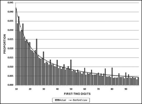
The usual approach is to use Access for the digit calculations and Excel for the tables and the graphs (first digits, second digits, and first-two digits). Excel can be used for the digit calculations for data tables that fit within its row limitations. There are nine possible first digits (1, 2, . . ., 9), 10 possible second digits (0, 1, . . ., 9), and 90 possible first-two digits (10, 11, . . ., 99). The first-two digit graph shown in Figure 5.2 is from an analysis of the digit frequencies of the invoice amounts for 2007 for a city in the Carolinas. The city government had about 250,000 transactions for the year. The fit to Benford's Law is excellent. The spikes that are evident at some of the multiples of 5 (15, 25, 30, 40, 50, 75, and 80) are quite normal for payments data.
Figure 5.2 The First Two Digit Frequencies of the Payments of a City Government. The X-Axis Shows the First Two Digits and the Y-Axis Shows the Proportions. The Line Represents the Expected Proportions of Benford's Law and the Bars Represent the Actual Proportions
The NigriniCycle.xlsx template includes a Tables worksheet. The Tables details include (a) the actual count for each digit combination, (b) the actual proportion and the expected proportion for each digit combination, (c) the difference between the actual and expected proportions, and (d) the Z-statistic for each digit combination (Z-statistics above 1.96 indicate that there is a significant difference between the actual and expected proportions).
The first digit test (not included in the NigriniCycle.xlsx template) is a high-level test of reasonableness that is actually too high-level to be of much use. This test can be compared to looking out the window of the plane when you are descending to land in your home city. One or two landmarks and the look of the terrain would be a reasonableness check that you are indeed landing at your home city. The general rule is that a weak fit to Benford's Law is a flag that the data table contains abnormal duplications and anomalies. If an investigator is working with four data tables and three of them exhibit a good fit to Benford's Law, then the strategy would be to focus on the fourth nonconforming data table because it shows signs of having the highest risks for errors or fraud. Similarly, if a single company had three quarters of conforming data and one quarter of nonconforming data, then the nonconforming data has the higher risk of errors or fraud.
The second-digit test is a second overall test of reasonableness. Again, this test is actually too high-level to be of much use. For accounts payable data and other data sets where prices are involved, the second-digits graph will usually show excess 0s and 5s because of round numbers (such as 75, 100, and 250). This is normal and should not be a cause for concern. If the second-digit graph shows an excess of (say) 6s, the suggested approach is to go to the first-two digits graph to check which combination is causing the spike (excess). The result might be that 36 has a large spike in which case the investigator would select and review a much smaller sample of suspect records. An example of a spike at 36 is shown in Figure 18.5 in Chapter 18.
The first-two digits test is a more focused test and is there to detect abnormal duplications of digits and possible biases in the data. A bias is a gravitation to some part(s) of the number line due to internal control critical points or due to psychological factors with respect to numbers. Past experience with the first-two digits graph has given us eight guidelines for forensic analytics:
1. A common finding when analyzing company expenses is a spike at 24. A spike is an actual proportion that exceeds the expected (Benford) proportion by a significant amount. This usually occurs at firms that require employees to submit vouchers for expenses that are $25 and higher. The graph would then show that employees are submitting excessive claims for just under $25.
2. Spikes at 48 and 49 and 98 and 99 indicate that there are excessive amounts that are just below the psychological cutoff points of $100, $500, $1,000, $5,000, or $10,000.
3. Spikes that are just below the first-two digits of internal authorization levels might signal fraud or some other irregularity. For example, an insurance company might allow junior and mid-level adjusters to approve claims up to (say) $5,000 and $10,000. Spikes at 48, 49, 98, 99 would signal excessive paid amounts just below these authorization levels.
4. Several years ago forensic investigators at a bank analyzed credit card balances written off. The first-two digits showed a spike at 49. The number duplication test showed many amounts for $4,900 to $4,980. Most of the “49” write-off amounts were attributable to one employee. The investigation showed that the employee was having cards issued to friends and family. The employee's write-off limit was $5,000. Friends and family then ran up balances to just below $5,000 (as evidenced by the spike at 49) and the bank employee then wrote the balance off. The fraud was detected because there were so many instances of the fraud and the person was systematic in their actions.
5. An auditor ran the first-two digits test on two consecutive months of cost prices on inventory sheets. The results showed that the digit patterns were significantly different. The investigation showed that many of the items with positive cost values in the first month erroneously had zero cost amounts in the second month.
6. A finding by Inland Revenue in the United Kingdom was that there was a big spike at 14 for revenue numbers reported by small businesses. The investigation showed that many businesspeople were “managing” their sales numbers to just below 15,000 GBP (pounds). The tax system in the United Kingdom allows businesses with sales under £15,000 to use the equivalent of a “Schedule C Easy” when filing.
7. Employee purchasing cards were analyzed at a government agency. The agency had a limit for any purchase by credit card of $2,500. The investigation showed a big spike (excess) at 24 due to employees purchasing with great gusto in the $2,400 to $2,499.99 range. This graph is shown in Figure 18.5. It was only because the proportions could be compared to Benford's Law that the investigators could draw the conclusion that the actual proportion was excessive. A result is only excessive when the investigator is able to compare the results to some accepted norm.
8. The accountants at a Big-4 audit firm tested their employee reimbursements against Benford's Law. The results for one employee showed a spike at 48. It turned out that the employee was charging his morning coffee and muffin to the firm every day, including those days when he worked in the office. One would think that an auditor would pay for his own breakfast!
The first-order test involves a set sequence of actions. The starting point is to calculate the first-two digits of each amount. Thereafter the first-two digits are counted to see how many of each we have. The results are then graphed and supporting statistics are calculated. The test is described in general terms in more detail below.
The first-two digit test is built into IDEA. In IDEA you would simply call up the routine and identify which field was the field of interest. To run the first-two digit test in Access or Excel requires a sequence of steps that are summarized below:
1. Use the Left function to calculate the first-two digits.
2. Use Where to set the >=10 criteria in the query. Because all numbers are >=10, we can use Left for the first-two digits. When analyzing negative numbers, we need to use the Absolute function to convert them to positive numbers.
3. Use a second query to count the number of times each first-two digit occurs. In Access this is done using Group By and in Excel this is done using COUNTIF.
4. If the calculations are done in Access, then the results need to be copied to the NigriniCycle.xlsx template so that the graphs and tables can be prepared. This template is also used if the calculations are done in Excel.
The above steps are an outline of how the tests would be run using Access or Excel. The actual mechanics are described in the next sections using the InvoicesPaid.accdb database. This database contains the invoices paid by a utility company. This is the same set of data that was used in Chapter 4.
Running the First-Two Digits Test in Access
In a forensic environment the first-order first-two digits test (hereinafter first-two digits test) would be run after the high-level overview tests of Chapter 4. Those tests were the data profile, the periodic graph, and the histogram. We would use the same database to continue with our tests. The first step would therefore be to open the InvoicesPaid.accdb database.
When the database is opened we are given a security warning that “Certain content in the database has been disabled.” Since we do not want the content to be disabled, the next step would be to click on the Options button. Thereafter select the radio button with the Enable this content option. Now click OK to get a database that is fully enabled and that does not have a security warning below the ribbon.
Our first query calculates the first-two digits of the Amounts. The first query is started with the usual Create→Other→Query Design. The invoices table tblInvoicesPaid is selected by selecting the table and then clicking Add followed by Close. The first-two digits of each number are calculated using a calculated field as is shown in Figure 5.3.
Figure 5.3 The Query Used to Calculate the First Two Digits of Each Number
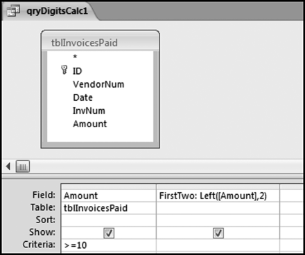
The query used to calculate the first-two digits of each number is shown in Figure 5.3. The field with the first-two digits is named FirstTwo. The formula is shown below:
FirstTwo:Left([Amount],2)
The square brackets [ ] indicate that the formula is referring to the field called Amount. The >=10 criteria is used because we only do the tests on numbers that are 10 or greater because numbers less than 10 are usually immaterial. The Left function works correctly because it is operating on numbers that are positive and 10 or more. To calculate the digits of negative numbers we would have to include the Absolute (Abs) function in our formula. The result of running this query is an output data set with 177,763 records showing all the >=10 amounts and their first-two digits. The total of 177,763 records agrees with the data profile in Figure 4.1. Save the query as qryDigitsCalc1 (an abbreviation for “digits calculate”) with a right click on Query1 and then by following the prompt for the query name. Close qryDigitsCalc1.
The second step is to count how many times each possible first-two digits combination occurred. The second query is a requery of qryDigitsCalc1 and we set this up by using the usual Create→Other→Query Design. The query qryDigitsCalc1 is selected by selecting the Queries tab and then selecting qryDigitsCalc1 followed by Add and then Close. The query used for the counting function is shown in Figure 5.4.
Figure 5.4 The Second Query Used for the First-Two Digits Test
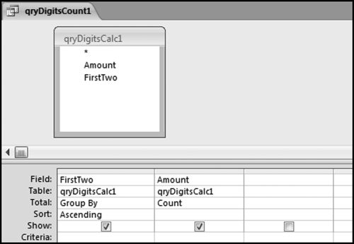
This query groups the first-two digits and counts how many times each combination occurred. The query is run using Design→Results→Run and the results are shown in Figure 5.5.
Figure 5.5 The Results of the Second First-Two Digits Query
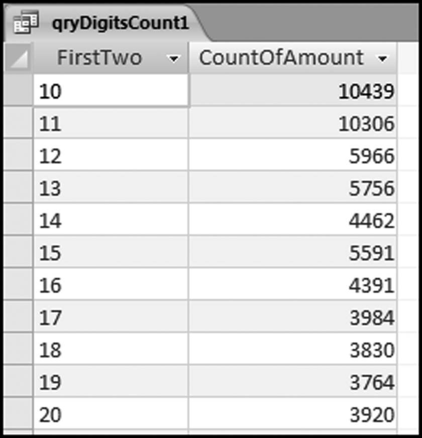
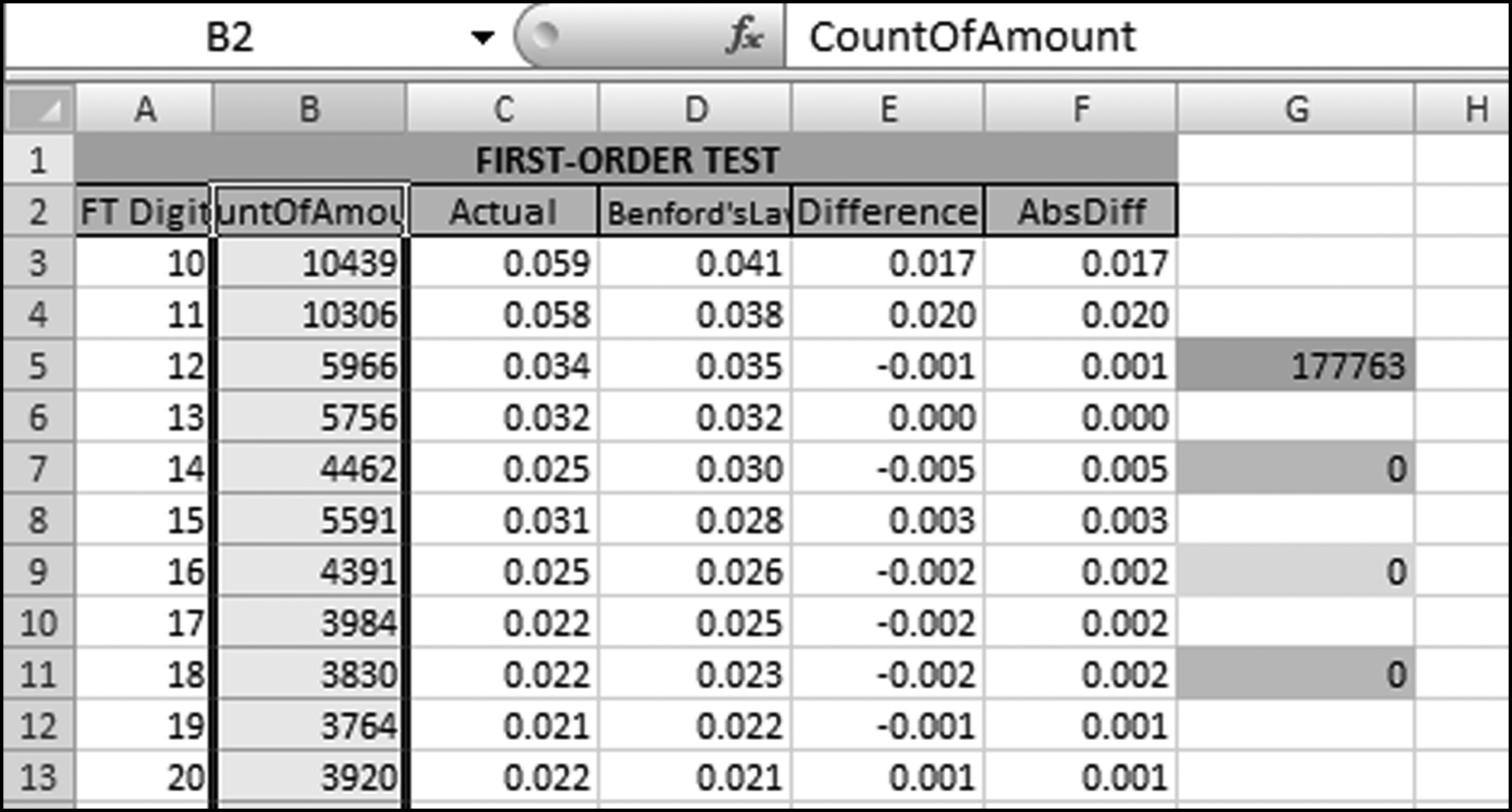
The result shows us that we had 10,439 records that had first-two digits of 10 for the Amount field and 10,306 records that had first-two digits of 11. We can see that we do not have a good fit to Benford's Law. There is a steep drop-off from 10 and 11 to 12. Viewing these results on a graph would allow us to see the spikes on the graph. We will use the NigriniCycle.xlsx template to prepare the graph. Open this file and click the Tables tab.
The CountOfAmount field in Figure 5.5 needs to be copied using the usual Copy and Paste functions to column B of the template starting in cell B2. The result of the Copy and Paste is shown in Figure 5.6.
Figure 5.6 Results of Pasting the Access Output into the Template
Columns C, D, E, and F as well as cell G5 is automatically recalculated. The template also automatically prepares the first-two digits graph. The graph is viewed by clicking on the FirstOrder tab. The first-two digits graph is shown in Figure 5.7.
Figure 5.7 The First-Two Digits Graph of the Invoicespaid Data
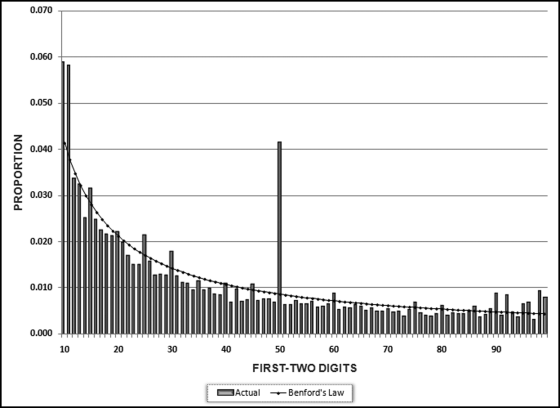
The first-two digits graph in Figure 5.7 shows a major spike at 50, and two other significant spikes at 10 and 11. We also notice the two spikes at 98 and 99. Although these might not seem to be large spikes, the actual proportions of 0.009 and 0.008 are about double the expected proportion of 0.004. Also, these two-digit combinations (98 and 99) are just below a psychological threshold and we should check whether the digits are for amounts of $98 and $99 (which are not too material) or $980 to $999 (which are material). The graph shows that we have an excessive number of invoices that are just below psychological thresholds.
The Excel template NigriniCycle.xlsx has some columns that are automatically calculated. The columns that relate to the first-order tests are columns A through F. An explanation for the columns that are automatically calculated is given below:
- Column B. The Count column shows the count of the numbers that had first-two digits of d1d2. In this case there were 10,439 numbers with first-two digits of 10.
- Column C. The Actual column shows the actual proportion of numbers that had first-two digits of d1d2. For the 10 combination the actual proportion of 0.059 is calculated as 10,439 divided by 177,763.
- Column D. The Benford's Law column shows the expected proportions of Benford's Law. The 90 Benford's Law proportions must sum to 1.000 and the 90 Actual proportions must also sum to 1.000. Small differences may occur due to rounding.
- Column E. The Difference column shows the difference between the actual proportion and the Benford's Law proportion. The difference is calculated as Actual minus Benford's Law. Positive differences tell us that the actual proportion exceeded the Benford's Law proportion.
- Column F. The AbsDiff column is the absolute value of the Difference in column E. These absolute values are used to calculate the Mean Absolute Deviation (MAD), which measures the goodness of fit to Benford's Law. The MAD is discussed further in Chapter 6.
Assessing the conformity (the goodness of fit) to Benford's Law is reviewed in Chapter 6. This case study is also continued in Chapter 6 and in others chapters that follow where we will home in on the suspect or suspicious transactions. For now, our conclusion is that our first order test has shown some large spikes at 10, 11, 50, 98, and 99. Running the tests in Excel is shown in a later chapter.
Benford's Law gives the expected frequencies of the digits in tabulated data. These expected digit frequencies are named after Frank Benford, a physicist who published the seminal paper on the topic (Benford, 1938). Benford analyzed the first digits of 20 lists of numbers with a total of about 20,000 records. He collected data from as many sources as possible in an effort to include a variety of data tables. His results showed that on average 30.6 percent of his numbers had a first digit 1, and 18.5 percent of his numbers had a first digit 2. Benford's paper shows us that in theory and in practice that the digits are not all equally likely. For the first (leftmost) digit there is a large bias in favor of the lower digits (such as 1, 2, and 3) over the higher digits (such as 7, 8, and 9). This large bias is reduced as we move from the first digit to the second and later digits. The expected proportions are approximately equal from the third digit onwards.
The Benford's Law literature started with three papers in the 1940s. A significant advance came in the 1960s when it was discovered that Benford's Law was scale invariant. This means that if the digits of the areas of the world's islands, or the length of the world's rivers followed a law of some sort, then it should be immaterial which measurement unit was used. Benford's Law was found to be scale invariant under multiplication and so if all the records in a table that conformed to Benford's Law were multiplied by a (nonzero) constant, then the new list would also follow Benford's Law. A list of numbers that conform to Benford's Law is known as a Benford Set.
Another significant theoretical advance came in the 1990s when Hill showed that if distributions are selected at random, and random samples are then taken from each of these distributions, then the digits of the resulting collection will converge to the logarithmic (Benford) distribution. Hill's paper explained why Benford's Law is found in many empirical contexts, and helps to explain why it works as a valid expectation in applications related to computer design, mathematical modeling, and the detection of fraud in accounting settings. The 1990s also saw practical advances in the use of Benford's Law. An early fraud study showed that the digit frequencies of the invented fraudulent numbers did not follow Benford's Law. The increased ease of computing allowed for more research on larger and larger data sets showing Benford's Law to be valid in a variety of financial and accounting contexts. In 1999 a Benford's Law paper was published in a widely circulating accounting journal and Benford's Law was then introduced to the accounting and auditing community.
A few general tests can be used to see whether Benford's Law is a valid expectation. The general considerations are that the data set should represent the sizes of facts or events. Examples of such data would include the populations of towns and cities, or the market values of listed companies. Also, there should be no built-in minimum or maximum values in the data table, except that a minimum of zero is acceptable. Finally, the data table should not represent numbers used as identification numbers or labels. Examples of these numbers are social security numbers, bank account numbers, and flight numbers. A final consideration is that there should be more than 1,000 records for Benford's Law to work well.
The chapter shows the queries used in Access to run the first-two digits test. An Excel template is used to prepare the graphs. The first-two digits test is a high-level overview. A weak fit to Benford's Law suggests a heightened risk of errors or fraud. The first-two digits test is also effective in identifying biases in the data. These biases could be excessive purchases just below a control threshold of (say) $2,500, or an excess of taxpayers reporting sales amounts just below 15,000 British pounds where this is the cutoff amount to file a simplified tax return.