Chapter 6
Benford's Law
Assessing Conformity
Chapter 5 reviewed the history of Benford's Law, some possible uses for the results of our tests, and how to run the first-two digits test in Access. The focus of this chapter is on ways to assess the conformity of a data set to Benford's Law. The focus of our attention is Benford's Law, but these methods can be used for conformity to other expected values. We have many statistical methods and the concept of significance so it would seem that assessing the goodness of fit of our data to Benford's Law is a straightforward matter. However, our task is complicated by the fact that we are usually dealing with large data sets where even small deviations from the expected pattern are statistically significant.
Prior to the mid-1990s there was not much of a need to address conformity criteria. Most research papers used relatively small data sets. An exception to this rule was Thomas (1989) who analyzed 69,000 positive earnings numbers and 11,000 negative earnings numbers. In his study the Z-statistic worked well for the test of the first-two digits. The chapter reviews the tests described in most statistics books that would work well for smaller data sets. Thereafter we examine some of the mathematical properties of Benford's Law and the “best” test is suggested based on these properties. The conformity tests are demonstrated using both Access and Excel.
For the first-two digit test there are two ways to look at conformity. The first way is to test whether a specific first-two digit combination follows Benford's Law. The second way is to test whether the digit combinations (10, 11, 12, . . . 99) combined follow Benford's Law. This distinction is the subject of an excellent paper by Cleary and Thibodeau (2005). There are, however, issues with each of these methods. This chapter reviews the Z-statistic, chi-square test, Kolmogorov-Smirnoff test, the Mean Absolute Deviation, the basis of Benford's Law, and a test called the mantissa arc test (which is only slightly less complicated than it sounds).
One Digit at a Time: The Z-Statistic
The Z-statistic is used to test whether the actual proportion for a specific first-two digit combination differs significantly from the expectation of Benford's Law. The formula takes into account the absolute magnitude of the difference (the numeric distance from the actual to the expected), the size of the data set, and the magnitude of the expected proportion. The formula adapted from Fleiss (1981) is shown in Equation 6.1:
where EP denotes the expected proportion, AP the actual proportion, and N the number of records. The (1/2N) term is a continuity correction term and is only used when it is smaller than the first term in the numerator.
From the numerator of Equation 6.1 we can see that the Z-statistic becomes larger as the difference between the observed (actual) proportion and expected proportion becomes larger. In the invoices table, the first-two digits 50 has an expected proportion of 0.009 and an actual proportion of 0.041. With 177,763 records in the table, the Z-statistic is calculated (using exact values) to be 149.333. At a significance level of 5 percent, the cutoff score is 1.96 and our calculated Z of 149.333 exceeds this cutoff score leading us to conclude that the actual proportion differs significantly from the expected proportion. At the 1 percent significance level our cutoff score would be 2.57, and we would have a significant difference if the calculated Z exceeded 2.57.
The second term in the Equation 6.1 numerator (1/2N) is a continuity correction factor and it usually has little impact on the calculated Z-statistic. The effect of N in the denominator is that as the data set becomes larger, so the Z-statistic becomes larger. So our difference of 0.033 becomes more and more significant as the data set increases in size. Using the same actual proportion, if the data set had 500,000 records the calculated Z-statistic would be 250.463. The number of records almost tripled, but the Z-statistic showed a much smaller increase because N is inside the square root sign.
The expected proportion, EP, appears twice in the denominator. The effect of EP is that for any given difference, a larger expected proportion gives a smaller Z-statistic. In the above example we have a 3.3 percent difference (0.041 – 0.009). If the expected proportion was (say) 50 percent, and the actual was 53.3 percent, we would still have a 3.3 percent difference. However, with a data set of 177,763 records the Z-statistic would be lower at 27.825, which is still above the cutoff score for a significant difference at the 1 percent level.
The effect of EP is quite logical. A 3.3 percent difference when EP is 4.1 percent means that the actual proportion is 3.80 times the expected proportion. However, when the expected proportion is 0.500 and the actual proportion is 0.533 there is a smaller relative difference between the two numbers. So any difference of x is more significant for the higher digits (which have lower expected proportions) than for the lower digits (which have higher expected proportions).
The Z-statistic tells us whether our actual proportion deviates significantly from the expected proportion. We usually use a significance level of 5 percent. The Z-statistic suffers from the excess power problem. For large data sets, even a small difference is likely to be flagged as significant. For example, for the InvoicesPaid data, 85 of the 90 first-two digit combinations have differences that are statistically significant. The large number of records makes small differences significant. The nonsignificant differences are for 13, 21, 40, 85, and 93. The Z-statistics taken together signal an extreme case of nonconformity.
For a larger data set of 1,000,000 records we might have an expected percentage of 10 percent for the second digit 4. If our actual percentage is 10.018 percent (a really small difference) the result is significant at the 0.05 level. With an expected percentage of 4 percent, an actual percentage of just 4.008 percent would be significant at the 0.05 level. This is indeed an insignificant difference from a practical perspective.
One solution is to ignore the absolute size of the Z-statistics. For the first-two digits there would be 90 Z-statistics (one for 10 through 99). Investigators would concentrate on which Z-statistics were both largest and associated with positive spikes (where the actual proportion exceeds the expected proportion). For the InvoicesPaid data the seven largest Z-statistics were for the 50, 11, 10, 98, 90, 92, and 99. These results will be considered in Chapter 8 in the number duplication test.
It is possible to calculate upper and lower bounds. These are the proportions at which the calculated Z-statistics equal 1.96. Any spike that protruded above the upper bound, or fell beneath the lower bound, would be significant at the 0.05 level. However, with the excess power problem we know that as the data table becomes larger, so the Z-statistic tolerates smaller and smaller deviations. Therefore, for large data tables, the upper and lower bounds will be close to the Benford's Law line. For very large data tables the lines will be so close to the Benford line that the upper and lower bounds might be indistinguishable from the Benford's Law line.
The Z-statistics cannot be added or combined in some other way to get an idea of the overall extent of nonconformity. So, a natural extension to the Z-statistic is a combined test of all the first-two digits. The well-known chi-square test and the Kolmogorov-Smirnoff test are discussed next.
The Chi-Square and Kolmogorov-Smirnoff Tests
The chi-square test is often used to compare an actual set of results with an expected set of results. Our expected result is that the data follows Benford's Law. The null hypothesis is that the first two digits of the data follow Benford's Law. The chi-square statistic for the digits is calculated as is shown in Equation 6.2:
where AC and EC represent the Actual Count and Expected Count respectively, and K represents the number of bins (which in our case is the number of different first-two digits). The summation sign indicates that the results for each bin (one of the 90 possible first-two digits) must be added together. The number of degrees of freedom equals K − 1 which means that for the first-two digits the test is evaluated using 89 degrees of freedom. The chi-square statistic (the sum of the 90 calculations) for the InvoicesPaid data equals 32,659.05.
The calculated chi-square statistic is compared to a cutoff value. A table of cutoff scores can be found in most statistics textbooks. These cutoff values can also be calculated in Excel by using the CHIINV function. For example, CHIINV(0.05,89) equals 112.02. This means that if the calculated chi-square value exceeds 112.02 then the null hypothesis of conformity of the first-two digits must be rejected and we would conclude that the data does not conform to Benford's Law. The higher the calculated chi-square statistic, the more the data deviate from Benford's Law. If our calculated chi-square statistic was 100, then in statistical terms we would conclude that there is not enough evidence to reject the null hypothesis. The null hypothesis is that there is no significant difference between the actual proportions and those of Benford's Law.
From Figure 5.7 we can see that the actual proportions of the InvoicesPaid data deviate quite radically from the expected proportions. We need not really use the Z-statistic results (that there are 85 significant differences) to quickly assess the situation. The chi-square statistic also suffers from the excess power problem in that when the data table becomes large, the calculated chi-square will almost always be higher than the cutoff value making us conclude that the data does not follow Benford's Law. This problem starts being noticeable for data tables with more than 5,000 records. This means that small differences, with no practical value, will cause us to conclude that the data does not follow Benford's Law. It was precisely this issue that caused the developers of IDEA to build a maximum N of 2,500 into their Benford's Law bounds. Their Benford's Law graphs show an upper and a lower bound (above or below which we have a significant difference) that is based on the actual number of records, or 2,500, whichever is smaller. This ensures that the graphical bounds are not too close to the Benford's Law line so that all digits and digit combinations show significant differences. The chi-square test is also not really of much help in forensic analytics because we will usually be dealing with large data tables.
Another “all digits at once” test is the Kolmogorov-Smirnoff (abbreviated K-S) test. This test is based on the cumulative density function. In Figure 5.6 we can see that the expected proportions for the first digits 10, 11, and 12 are 0.041, 0.038, and 0.035, respectively. The cumulative density function is the cumulative sum of these values, which is 0.041 (the first proportion), 0.079 (the sum of the first two proportions), and 0.114 (the sum of the first three proportions), and so on to the 90th proportion. The third cumulative sum means that the expected probability of 10s, 11s, and 12s taken together is 0.114. For the InvoicesPaid data the sum of the actual 10, 11, and 12 proportions is 0.150. We get this by adding the actual proportions for 10, 11, and 12. At 12, we have an expected cumulative proportion of 0.114 and an actual cumulative proportion of 0.150. The difference between the expected and the actual cumulative proportions is 0.036. The K-S test takes the largest of the absolute values of these 90 possible first-two digit differences (called the supremum in statistical terms). The formula to determine whether the result is significant is shown in Equation 6.3:
where 1.36 is the constant for a significance level of 0.05, and N is the number of records.
For the InvoicesPaid data there are 177,763 records and so the calculated K-S cutoff value is 1.36/sqrt(177763), which equals 0.00323. From the previous paragraph we know that the difference between the expected and actual cumulative proportion at 12 is 0.036. We need not go any further. Our difference of 0.03632 exceeds the K-S cutoff of 0.00323 and we have only looked at one cumulative difference. The null hypothesis that the data follows Benford's Law is rejected. A line graph of the actual and expected cumulative density functions is shown in Figure 6.1.
Figure 6.1 The Cumulative Density Function of Benford's Law and the Cumulative Density Function of the Invoices Data
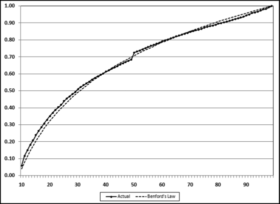
The two cumulative density functions in Figure 6.1 seem to track each other closely. Once again the excess power problem means that while matters might look quite good visually, only small deviations are tolerated when the number of records becomes large. The supremum (the largest difference) occurs at 11. The kink upward at 50 is because of the large spike at 50. Both cumulative density functions end at 1.00. The inclusion of N in the formula makes the K-S a weak choice in a forensic analytics setting.
The Mean Absolute Deviation (MAD) Test
The Mean Absolute Deviation (MAD) test ignores the number of records, N. The MAD is calculated using Equation 6.4:
where EP denotes the expected proportion, AP the actual proportion, and K represents the number of bins (which equals 90 for the first-two digits).
A version of the MAD (based on the percentage error) is used in time-series analysis where it is used to measure the accuracy of fitted time-series values. A low level of error indicates that the fitted time series values closely approximate the actual values and that the forecast can be seen to be reliable. Minitab calculates the MAD and also two other accuracy measures for time-series analysis. Since the MAD measures the accuracy in the same units as the data (in our case the proportions) it is easier to understand this measure. The number of records is not used in Equation 6.4.
There are three parts to the MAD. The numerator measures the difference between the actual proportion and the expected proportion for each first-two digit proportion. For the InvoicesPaid data we have an actual proportion of 0.059 for the 10 and an expected proportion of 0.041 for the 10. The deviation is the difference between the two numbers, which is 0.017. The absolute function means that the deviation is given a positive sign irrespective of whether the deviation is positive or negative. The absolute deviation of 0.017 can be seen in column F of Figure 5.6. The numerator of Equation 6.4 calls for us to sum the 90 first-two digit absolute deviations. The denominator tells us to divide by the number of bins, which is 90. This will give us the average (or mean) absolute deviation. When we apply the formula to the InvoicesPaid data we get a MAD of 0.00243. The MAD is therefore the average deviation between the heights of the bars in Figure 5.7 and the Benford line in Figure 5.7. The higher the MAD, the larger the average difference between the actual and expected proportions.
The NigriniCycle.xlsx template calculates the absolute deviations in column F. The MAD can be calculated by calculating the average for cells F2:F92. The MAD seems to be our answer. Unfortunately there are no objective statistically valid cutoff scores. We do not know what constitutes a big MAD that signals that our data does not conform to Benford's Law. Drake and Nigrini (2000) offer some suggestions based on their personal experiences. Their guidelines are based on everyday data sets that were tested against Benford's Law. Their table is due for an update and Figure 6.2 shows the Excel spreadsheet summarizing the MAD results of an analysis of 25 diverse data sets.
Figure 6.2 An Analysis of 25 Diverse Data Sets Where Conformity to Benford's Law Ranged from Near Perfect to Nonconformity
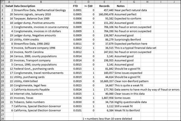
Based on these results a new set of first-two digits cutoff values was developed. These MAD cutoff values are shown in Table 6.1.
Table 6.1 The Cutoff Scores and Conclusions for Calculated MAD Values.
| First-Two Digits MAD Range | Conclusion |
| 0.0000 to 0.0012 | Close conformity |
| 0.0012 to 0.0018 | Acceptable conformity |
| 0.0018 to 0.0022 | Marginally acceptable conformity |
| Above 0.0022 | Nonconformity |
The MAD of the InvoicesPaid data is 0.00243 and the conclusion is therefore that the data set does not conform to Benford's Law. This is a reasonable result given that we can see several large spikes in Figure 5.7 and the clear nonconformity signals from the Z-statistics, the chi-square test, and the K-S test.
Tests Based on the Logarithmic Basis of Benford's Law
Figure 5.1 in Chapter 5 showed that the mathematical basis of Benford's Law is that the data, when ranked from smallest to largest, forms a geometric sequence. A geometric sequence is one where each term after the first term is a fixed percentage increase over its predecessor. The usual mathematical representation for such a sequence is given by
(6.5)
where S denotes the sequence, a is the first term in the sequence, r is the common ratio, and n denotes the nth term. In Figure 5.1, a equals 10, r (the common ratio) equals 1.002305, and there are 1,000 terms in the sequence.
Raimi (1976) notes that the data need only approximate a geometric sequence. For example, the Fibonacci sequence (1, 1, 2, 3, 5, 8, . . .) conforms closely to Benford's Law if the data table is large enough. A little bit of arithmetic and some knowledge of logarithms (to the base 10) is needed over here. The log of a number (base 10) is derived as follows:
Equations 6.6 and 6.7 show us that 2 is the log (base 10) of 100 because 102 equals 100. Also, 2.30103 is the log (base 10) of 200 because 102.30103 equals 200. Note that 0.30103 is the expected probability of a first digit 1 (see Table 5.1). Also, 2.47712 is the log (base 10) of 300 because 102.47712 equals 300. Note that 0.47712 is the combined (cumulative) probability of the first digit being either a 1 or a 2. A well-known property of logarithms is shown in Equation 6.8:
The result of the property in Equation 6.8 is that the logs (base 10 will always be used unless stated otherwise) of a geometric sequence will form a straight line. In an arithmetic sequence the difference between any two successive numbers is a constant. In our case these differences will be the log of r, the common ratio. As a preliminary test of this property and the “Benfordness” of our InvoicesPaid data we will graph the logs of the sequence that is formed by ordering our data from smallest to largest. We will need a two-step procedure because we cannot graph 177,763 data points in Excel. Excel's graphing limit is 32,000 data points. Our strategy is therefore to calculate the logs of the numbers in the Amount field and then to plot every sixth record, which will give us a good enough picture of the logs of our data.
The above is quite straightforward except for the wrinkle that Access cannot directly calculate the log (base 10) of a number. Access can calculate the log to the base e (abbreviated ln). We therefore need to use Equation 6.9 below to convert the natural logarithms to logs to the base 10.
A final consideration is that the log of a negative number is undefined (it does not exist) and the general approach for accounts payable data is to ignore numbers less than $10 for the first-order test. We will also ignore these small amounts on our log graphs. We therefore need to restrict the log calculations to amounts >=10. A minimum value that is an integer power of 10 (101, 102, 103, and so on) should not upset the digit patterns or the log graph. The first query calculates the log (base 10) using Equation 6.9 and it adds a new field that is a random number from 0 to 1. This query is shown in Figure 6.3.
Figure 6.3 The Query Used to Calculate the Logs and to Extract a Random Sample of Records
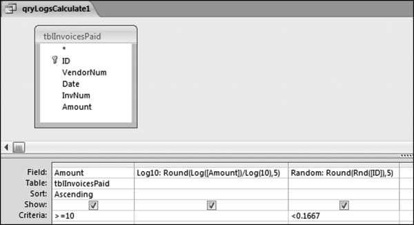
The query to calculate the logs and to extract a random sample of about one-sixth of the records is shown in Figure 6.3. The query only calculates the logs for amounts >=10. The calculated fields are:
Log10:Round(Log([Amount])/Log(10),5)
Random:Round(Rnd([ID]),5)
The Log10 field calculates the log of each amount. The log is rounded to five places to keep the results tidy. The second calculated field, Random, creates a random number, rounded to five places, using the ID field as a seed value. The < 0.1667 criteria randomly keeps about one-sixth of the records (1/6 is about 0.1667). The query would also work if the criteria was a range such as “Between 0.40 and 0.5667.” This query will produce the same random sample each time Access is started and the InvoicesPaid database is opened and the query is run. After the query is run Access recalculates the random numbers and so the random numbers in the output are once again random (from 0 to 1) and are not all less than 0.1667. Save the query as qryLogsCalculate1. The query returns a table of 29,662 records. This number might or might not differ from computer to computer and from Access version to Access version. The result will, however, always be close to 29,662 records.
The next step is to graph the logs in Excel. The shape of the graph of 29,662 records should closely mimic the patterns in the full data set of 177,763 records. Copy the contents of the Log10 field (using Copy and Paste) from Access to the Logs tab in column B of the NigriniCycle.xlsx template. Populate the Rank field with a series of numbers starting with 1 and ending with 29,662 at the last record (on row 29,663). The result is shown in Figure 6.4.
Figure 6.4 The Log and Rank Data Used to Graph the Ordered Logs
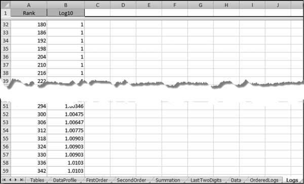
The ordered log data is shown in Figure 6.4. The logs should now be graphed using Excel's graphing capabilities. The first step is to highlight the range containing the data to be graphed, namely B2:B29663. The graph is then prepared using Insert→Charts→Line. The resulting graph after a little bit of formatting is shown in Figure 6.5.
Figure 6.5 The Ordered (Sorted) Logs of the InvoicesPaid Data
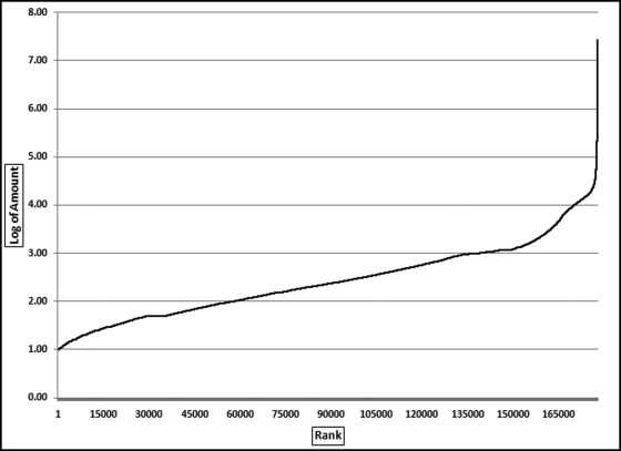
The graph shows a reasonably straight line through to rank 150000, after which we get another (almost) straight line with a steeper slope through to the end. The sharp upward curve on the right side of the graph is due to a handful of items that would have little impact on any goodness of fit test. We can see a horizontal segment at about 1.70 and again at 3.00. These are due to excessive duplications of $50 and numbers around $1,000 and higher. The horizontal segment at around 1.7 is associated with the large spike visible at 50 in Figure 5.7.
If the data followed Benford's Law closely we would see either a single straight line, or a series of straight lines with varying slopes from integer value to integer value. That is, from 1.00 to 2.00, from 2.00 to 3.00, from 3.00 to 4.00, and so on up the y-axis. The graph need not be straight (linear) from the first record to the Nth record, it need only be linear between the integer values on the y-axis. Also, if a linear segment has relatively few records (such as 4.00 to 5.00) then its effect on the digit frequencies is quite minor. For the invoices data the convex curved pattern from 1.00 to 2.00 probably has the most pronounced effect on the digit frequencies, followed by the 3.00 to 4.00 segment. Converting the logs back to numerical values this means that the biggest nonconforming segments are amounts from 10.00 to 99.99 and 1,000.00 to 9,999.00, respectively.
We are almost ready to use the logarithmic basis of Benford's Law to test for conformity. For the next step we need to go back to the 1880s to the very first paper on digital frequencies written by Newcomb (1881). Newcomb states that the frequency of the digits is based on the fact that their mantissas are equally probable. This is almost equivalent to our prior statements that the logs of the ordered data should follow a straight line. By way of example, we could have the logs forming a straight line from 1.302 to 1.476 on the y-axis. This data set would not conform to Benford's Law because all the numbers would range from 200 to 300 and we would have no numbers with a first digit 1, 3, 4, 5, 6, 7, 8, and 9. The requirement that the mantissas are uniformly distributed is more comprehensive (except that it ignores the negative numbers that we encounter in private and public data). The mantissa is described in Equations 6.10 and 6.11.
The mantissa is the fractional part of the log of a number. The mantissa is the part of the logarithm to the right of the decimal point and the characteristic is the integer part to the left of the decimal point. The characteristic is 2 in Equation 6.10. Mantissas can span the range [0,1). The square bracket and round bracket mean that zero is included in the range together with all values up to, but not including, 1. A set of data that conforms to Benford's Law is known as a Benford Set. A test of the mantissas can therefore be used as a test for a Benford Set. We need to test whether the mantissas are uniformly (evenly) distributed over the [0,1) interval. If the mantissas are distributed U[0,1) then the data conforms to Benford's Law. The query to calculate the mantissas uses the same logic as the query to calculate the logs. The query to calculate the mantissa is shown in Figure 6.6.
Figure 6.6 The Query Used to Calculate the Mantissas and to Extract a Random Sample of the Records
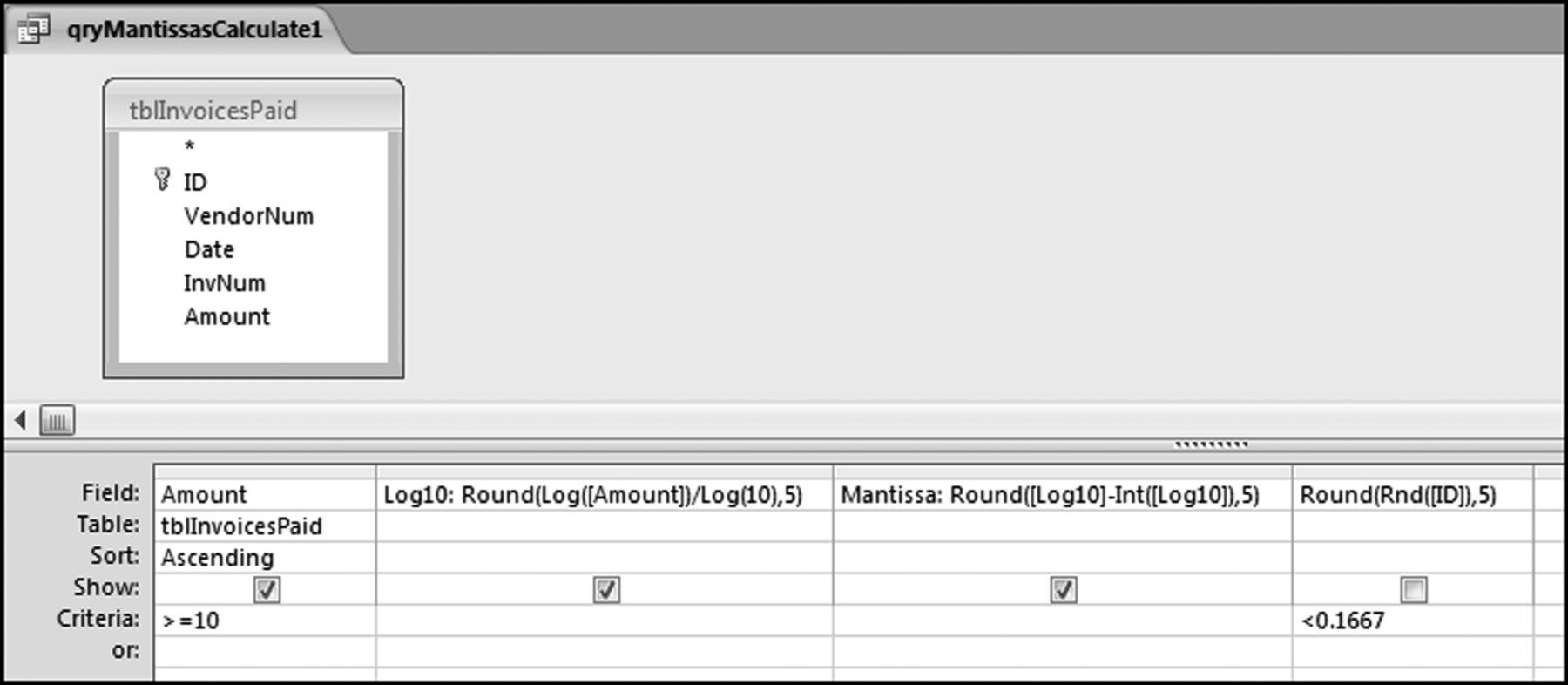
The query used to calculate the mantissas and to extract a random sample of one-sixth of the records is shown in Figure 6.6. This query follows the query in Figure 6.3 and includes a calculation of the mantissa. The mantissa formula is
Mantissa: Round([Log10]-Int([Log10]),5)
The Random field is not shown in the results because it is not needed in the result. The Round function is used to keep the results neat and tidy.
The data needs to be copied to Excel and the mantissas need to be sorted from smallest to largest. The graph of the ordered mantissas is prepared in Excel. The result for the InvoicesPaid data is shown in Figure 6.7 together with the dashed line that would be the plot for uniformly distributed mantissas.
Figure 6.7 The Ordered Mantissas of the Data and a Straight Line from 0 to 1
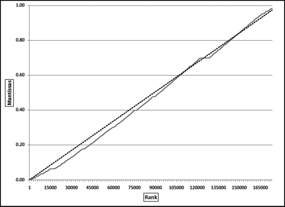
A necessary condition to test the mantissas for U[0,1) is that the mean is 0.50 and that the variance is 1/12. These conditions are, however, not sufficient conditions. Data sets that satisfy only the mean and variance requirements might have little or no conformity to Benford's Law. The basis of any mantissa-based model is that the ordered (ranked) mantissas should form a straight line from 0 to 1 (or more precisely (N-1)/N, which is fractionally less than 1) with a slope of 1/N. This is the dashed line in Figure 6.7. It is tempting to use regression to assess the goodness of fit. The quantile(Q-Q) plots of Wilk and Gnanadesikan (1968) also look promising. For a regression test we would only need to test the intercept (which would equal zero for perfect conformity), the slope (which would equal 1/N for perfect conformity, and the R-squared (which would equal 1 for perfect conformity). This test is the subject of research in progress. The next approach is the Mantissa Arc solution based on mantissas and another graphical approach. The Mantissa Arc test is described after we discuss how one can create a perfect Benford Set.
Creating a Perfect Synthetic Benford Set
Evaluating the possible goodness-of-fit tests for Benford's Law means that we should be able to create a perfect Benford Set against which to compare our results. From the previous section we know that the mantissas of a Benford Set are distributed uniformly (evenly) over the [0,1) range. One way to create a Benford Set is to create a set of uniform [0,1) mantissas and then to create a set of numbers from the mantissas.
Let us assume that we want to create a table with 1,000 numbers that range from 10 to 1,000. The lower bound is 10 and the upper bound is 1,000. To start we need to calculate d, which is the difference between the logs of the upper and lower bounds. This calculation is shown in Equation 6.12. Note that this difference must be an integer value (1, 2, 3, . . .) to give a Benford Set.
The mathematical representation for a geometric sequence is given in Equation 6.13.
where a is the first term in the sequence (in this case 10), r is the common ratio, and n denotes the nth term.
We need to calculate r, the common ratio that will give us a geometric sequence of exactly 1,000 terms that will start at 10 and end at 1,000. This is done using Equation 6.14.
Substituting N=1000 and d=2 in Equation 6.14 we get a calculated r of 1.00461579. The sequence can then be created in Excel as is shown in Figure 6.8.
Figure 6.8 The Creation of a Synthetic Benford Set
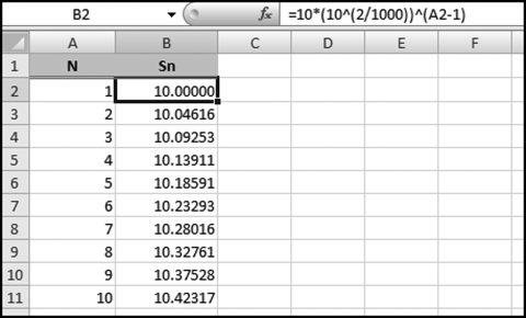
The first 10 records of the synthetic Benford Set is shown in Figure 6.8. The “10” in the formula bar is the a in Equation 6.13, the “10 (2/1000)” term is r from Equation 6.14, and the “A2-1” term is n – 1 from Equation 6.13. The synthetic (simulated) Benford Set has all the required attributes. The sequence stops just short of 1,000. As N gets larger, so the upper bound tends toward, but never exactly touches, the stated upper bound (of 1,000). A graph of the sequence will be a perfect geometric sequence. A graph of the logs will be a straight line from 1 to 3, and a graph of the mantissas will be a perfect straight line from 0 to 1. The Z-statistics will all be insignificant (some deviations will occur because 1,000 records cannot give us some of the exact Benford probabilities), the sequence will conform to Benford's Law using the chi-square test (where the calculated chi-square statistic is 7.74) and the K-S test (where the largest difference equals 0.00204). The MAD equals 0.00068, which is clearly close conformity. Our synthetic Benford Set is about as good as it can get for a table of 1,000 records. As N increases, so the fit will tend to be an even closer level of perfection.
Figure 6.7 shows the mantissas ordered from smallest and plotted as a straight line. If the data formed a Benford set the mantissas would be uniformly (evenly) distributed over the [0,1) range. No formal test related to the mantissas was proposed. Alexander (2009) proposes a test based on the mantissas, which we call the Mantissa Arc (MA) test.
In Figure 6.7 each mantissa is given a rank with the smallest value given rank #1 and the largest value given rank #N. The numeric value of the mantissa is plotted on the y-axis. In contrast, in the MA test each numeric value is plotted on the unit circle and for a Benford Set we would have a set of points uniformly distributed on the circle with radius 1 and centered on the origin (0,0).
Without showing the calculations just yet, the result that we would get for the Benford Set in Figure 6.8 would be as is shown in Figure 6.9.
Figure 6.9 A Set of Points on the Unit Circle and Centered at the Origin (0,0)
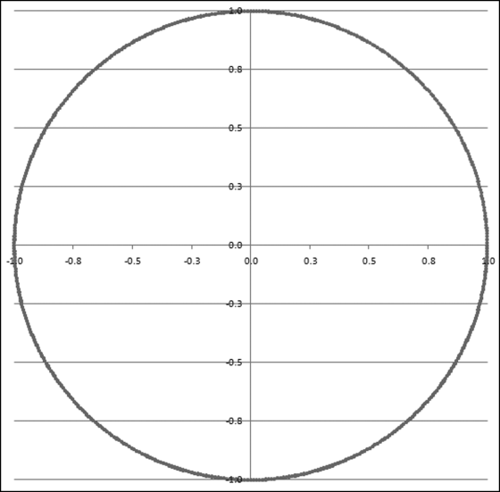
In Figure 6.9 the uniformly distributed mantissas have been converted (using formulas) to a set of uniformly distributed points on the unit (radius = 1) circle centered on the origin (0,0). Alexander then takes this concept further. He calculates the “center of gravity” inside the circle and then he calculates whether this center of gravity differs significantly from (0,0). This is very clever. If the center of gravity differs significantly from (0,0) then the points are not evenly distributed on the unit circle and the data is then not a Benford Set. The center of gravity must lie somewhere within the circle. An exception would be if we had a single point, in which case the center of gravity would also be that point. But with a single point we would not really even have a part of a circle. It would just be a point. To see what would happen if we had sections completely missing from our geometric sequence, the MA result is shown in Figure 6.10 for the case where we have a subset of a Benford Set, these being all the numbers from 10 to 19.999 and 50 to 59.999.
Figure 6.10 The Mantissa Arc Plot of 10 to 19.999 and 50 to 59.999
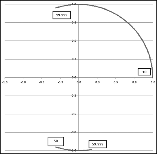
The circumference of a circle is 2πr and because we are dealing with the unit circle (where r equals 1) our circumference is simply 2π. This circumference of 2π equals 6.2832. The length of the arc in the top right quadrant (usually called quadrant I) extending into quadrant II is 1.8914, which equals (not by coincidence) 0.30103 (the first digit 1 probability) times 6.2832 (the circumference). The length of the arc in the neighborhood of (0, −1) that extends from quadrant III to quadrant IV is 0.4975, which is 0.07918 (the first digit 5 probability) times 6.2832. The MA method plots the uniformly distributed mantissas uniformly on the unit circle centered at the origin (0,0). A mantissa of 0 (which corresponds to a log of 1.000 or 2.000 and consequently a number equal to 10 or 100) is plotted at (1,0). A number such as 17.783 (or 177.83) would have its mantissa of 0.25 plotted at (0,1). A number such as 31.623 (or 3,162.3) would have its mantissa of 0.50 plotted at (−1,0). A number such as 56.234 (or 562,234) would have its mantissa of 0.75 plotted at (0,−1).
If the mantissas are uniformly distributed on the circle, then the center of gravity is the origin (0,0). Let our table of N records be denoted x1, x2, x3, . . ., xN. Each number must be converted to a point on the unit circle. The x-coordinate and the y-coordinates of the point are calculated as is shown in Equations 6.15 and 6.16.
where cos and sin refer to the trigonometric functions cosine and sine. The log is taken to the base 10 and mod 1 means that we only take the fractional part (the part to the right of the decimal point) of the log. For example, 11.03 mod 1 equals .03. The x-coordinate is sometimes called the abscissa and the y-coordinate is sometimes called the ordinate.
The center of gravity is also called the mean vector (MV) and its x and y coordinates are calculated as is shown in Equations 6.17 and 6.18.
The length of the mean vector, L2, is calculated as is shown in Equation 6.19 (which uses Equations 6.17 and 6.18).
Finally, the p-value of L2 is calculated using either Equation 6.20 or its algebraic equivalent in Equation 6.21.
Equation (6.21) shows us that as L2 or N get larger (mathematicians would say as they tend to infinity) so the p-value tends to 1.00. This is because as either L2 or N gets larger, the right-hand term tends toward zero and 1 minus zero equals 1.00. The p-value calculation is based on the tail of the chi-squared distribution with 2 degrees of freedom.
The calculations in Equations 6.17 to 6.21 were done in the lower part of the same Excel spreadsheet shown in Figure 6.8.
The mean vector and p-value calculations are shown in Figure 6.11. The Excel formulas are not too complicated especially when we realize that Equations 6.17 and 6.18 are simply telling us to take the average, and the mathematical constant e is the EXP function in Excel. The Excel formulas are
F1004: = AVERAGE(F2:F1001)
G1004: = AVERAGE(G2:G1001)
F1007: = F1004ˆ2+G1004ˆ2
F1010: = 1−EXP(−F1007*1000)
Figure 6.11 The Mean Vector and P-Value Calculations
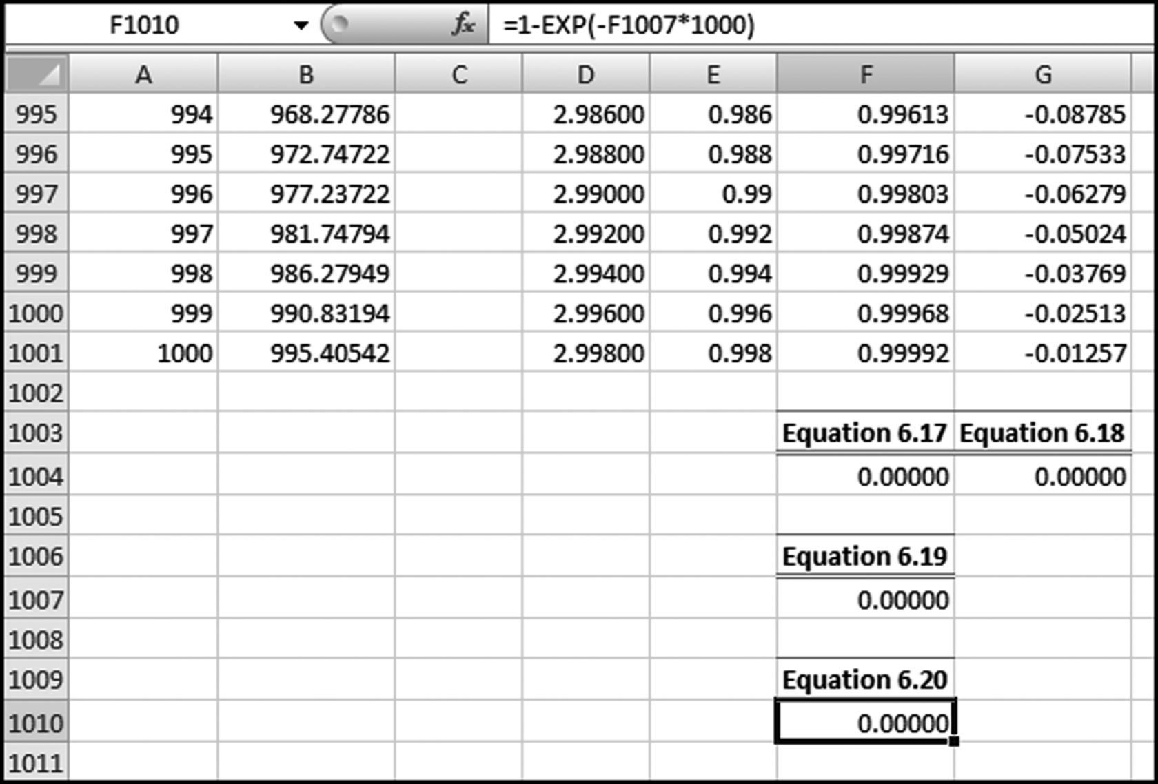
Since the calculated p-value in F1010 is less than 0.05, the null hypothesis of uniformly distributed mantissas is not rejected and we conclude that the data conforms to Benford's Law.
Going back to our InvoicesPaid data we would do the calculations by extracting a sample of about one-sixth of the records using the query in Figure 6.6. For this test we would only need to keep the field Amount in the result. The next step would be to paste the 29,662 amounts into an Excel spreadsheet and to calculate the mean vector and the p-value as is done in Figure 6.11. The calculations for the InvoicesPaid data are shown in Figure 6.12.
Figure 6.12 The Mean Vector and p-Value Calculations for the InvoicesPaid Data
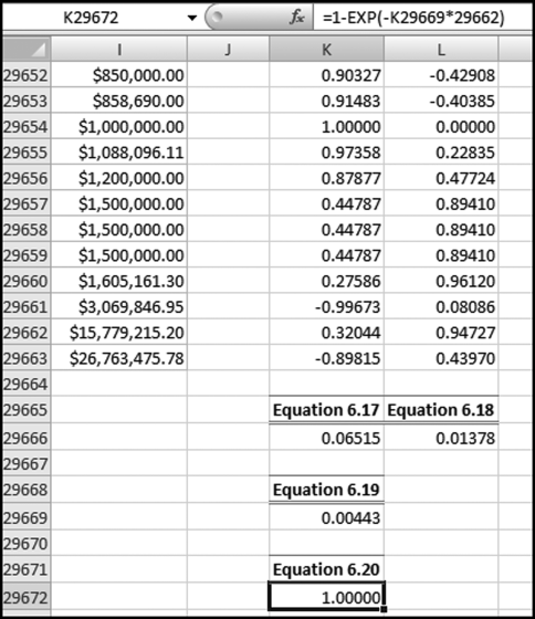
The length of the mean vector (the center of gravity) is 0.00443. This is based on a sample, but for a sample of 29,662 records the sample mean is for all practical purposes equal to the mean. The p-value of 1.00 indicates that the data does not conform to Benford's Law (which is in agreement with the Z-statistics, chi-square, K-S, and the MAD). If the p-value was less than 0.05 we would have to redo the calculations based on the whole population to see whether the p-value stays below 0.05 with a larger N.
The mantissa arc graph for the InvoicesPaid data together with the mean vector is shown in Figure 6.13. The graph was prepared in Excel.
Figure 6.13 The Mantissa Arc Graph and the Mean Vector for the InvoicesPaid Data
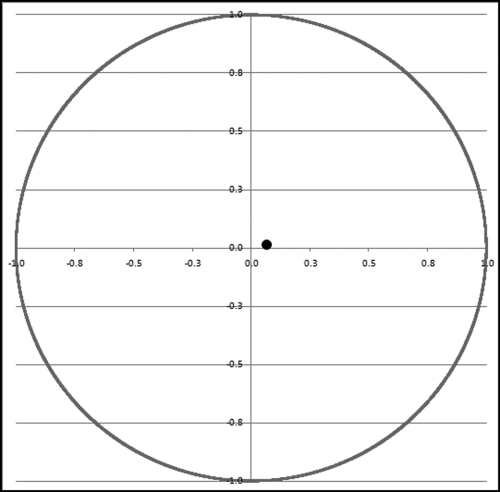
From the uniformity of the circle the data would seem that we have a good fit. However, what the graph actually shows us is that we are using all the points on the circle, or that all the mantissas seem to be used. There seem to be no open spaces between the markers (Excel terminology for points or dots) on the graph. If we used a fine marker (very small dots) we might see some open space. Unfortunately our markers are quite large and because we are plotting in two dimensions we cannot see how many markers are plotted on the same spot. The number 50.00 is used abnormally often in this data set. This corresponds to the point (−0.315, −0.949) in quadrant III. In this two-dimensional graph we cannot see that this point is plotted excessively often. Future research might point us in the direction of a three-dimensional graph.
The problem with the mantissa arc approach is that the length of the mean vector (equation 6.19) needs to be very small for the test to signal conformity through a p-value less than 0.05. For example, all the hypothetical situations in Table 6.2 would have a p-value in excess of 0.05 (signaling nonconformity).
Table 6.2 A Series of Hypothetical Results and the Mantissa Arc Test's Conclusions.

The mantissa arc test is offered as an interesting alternative test and also because it offers some interesting insights into the mathematical basis of Benford's Law. Future research in the area should address the very small tolerance for deviations from a mean vector length of zero. Perhaps using some rules of thumb much like was done with the Mean Absolute Deviation and Figure 6.2 and Table 6.1 we could end up with a Mantissa Arc table similar to Table 6.1. Alternatively researchers could leave the mantissa arc logic and method intact and substitute  or some smaller root to take account of the practical issues encountered with real world data sets.
Several valid goodness of fit tests are discussed in statistics textbooks. A major issue with each of these methods is that they work well for small data tables. When working with Benford's Law we often have large data tables and the usual test statistics always signal nonconformity. The basis of the classical tests is that we have a table of data that conforms to Benford's Law and from this we then extract a sample of x records. As the sample size increases so this mythical sample will tend towards conforming exactly to Benford's Law because the sample was drawn from a population that conformed to Benford's Law. These classical statistical methods “tolerate” only small deviations from perfection for large data sets.
We can assess conformity of a data set one digit at a time or all digits taken together. The Z-statistic is used to evaluate the digits one at a time. The test is based on both the absolute magnitude of the deviation and N, the number of records. As expected, this test suffers from the excess power problem in that even small deviations are statistically significant for large N. Both the chi-square and Kolmogorov-Smirnoff (K-S) tests evaluate all the digits at the same time. The chi-square test indirectly takes N into account. The K-S test incorporates N in the assessment of the significance of the result. In both cases the tests tolerate only small deviations from Benford's Law for large N making them only useful for comparing similarly sized data sets across time.
The Mean Absolute Deviation (MAD) test ignores N in its calculations thereby overcoming the problem related to large data sets. A problem with this test is that there are no objective cutoff values. A set of guidelines is offered based on an analysis of 25 real-world data sets.
The chapter reviewed the logarithmic basis of Benford's Law, which is that the mantissas (the fractional part of the logs) of the numbers are expected to be uniformly (evenly) distributed over the range [0,1). The square bracket means that the range includes 0 and the rounded bracket means that the range gets close to, but never actually touches 1. Some tests might be developed at some time in the future based on the logarithmic basis and the tools of linear regression. The chapter reviewed the mechanics of creating a synthetic (simulated) Benford Set being a set of numbers that conforms to Benford's Law. These data sets can be used by practitioners and researchers wanting to test various conformity methods, and for recreational Benford's Law research. The Mantissa Arc (MA) test of Alexander (2009) was reviewed. This clever technique transforms each number to a point on the unit circle centered at (0,0). The fit to Benford's Law is based on the distance of the center of gravity from (0,0) and N. Unfortunately this theoretically sound test is also sensitive and tolerates only very small deviations from Benford's Law.
Further research into conformity tests for large data sets is encouraged. The best solution seems to be the Mean Absolute Deviation (MAD). The cutoff values given in the chapter were based on the deviations found in several large real-world data tables.
