Chapter 16
Examples of Risk Scoring with Access Queries
Chapter 15 discussed the risk-scoring approach and the use thereof at a fast-food franchising company. This chapter is a continuation of the previous chapter with a review of other applications and an Access example. The chapter reviews the audit selection process used by the Internal Revenue Service (IRS) to demonstrate a highly sophisticated selection system. Other examples of the risk-scoring method are then reviewed. The examples include a banking fraud application, an airline ticketing fraud application, and a fictitious vendor fraud application. An example with financial statement fraud is presented in Chapter 17. The chapter concludes with an Access example showing a risk-scoring system designed to detect fraudulent vendors. Also discussed are general issues with using Access for these applications.
The risk-scoring model draws on the theory underlying decision-making cues. Using a psychology analogy, the predictors are the same as cues for decision making and the predictor weights are the same as the weights given to the decision-making cues. These weights have been addressed in psychological research studies. An early reference is Slovic (1966) in which he notes that little is known about the manner in which human subjects combine information from multiple cues, each with a probabilistic relationship to a criterion, into a unitary judgment about that criterion.
Slovic (1966) noted that a set of cues was consistent if the judge (decision maker) believed that the cues all agreed in their implications for the attributes being judged. Inconsistent cues would arise if the inferences that would be made from a subset of these cues would be contradicted by the conclusions from another set of cues. Consistency was seen to be a matter of degree and not an all-or-none matter. When a set of cues is consistent, each cue will be combined additively to reach a judgment. Inconsistent cues present a problem because in order to reconcile apparently contradictory information, the judge must either doubt the reliability of the cues or the belief in the correlation between the cues and the attributes being judged. In the risk-scoring method contradictory cues would occur if one cue indicated a positive risk of fraud and another cue signaled “no fraud” with certainty. The predictors are used to assess the risk of fraud and 0 and 1 simply indicate low risk and high risk as opposed to certainty.
The Audit Selection Method of the IRS
One of the largest fraud detection applications is the system used by the IRS to detect tax evasion. A review of their system is valuable because it shows what can be done if cost is not that much of a concern. The IRS reviews its system in IRS (1979, 1989). The system uses discriminant analysis and requires a special audit called the Taxpayer Compliance Measurement Program (TCMP) of thousands of taxpayers on a regular basis.
The first step in the audit selection process is the TCMP that uses a stratified sample of approximately 50,000 income tax returns (IRS 1989, 24). Taxpayers are subjected to an intensive audit, and are subject to penalties and additional taxes in the event of noncompliance. The cost of the 1985 TCMP was $128 million. Of this amount, $42 million was the direct cost, and $86 million was an opportunity cost because the revenue yield from the random selection process is below that of the systems usually used to select returns for audit.
The IRS believes that the TCMP provides value because it provides them with an estimate of the level of noncompliance, the noncompliance trend, and the characteristics of delinquent returns. The results are used to improve efficiency and effectiveness in numerous areas, including the selection of returns for audit and general tax administration policy and systems (IRS 1989, 1). The steps in developing the audit selection process (IRS 1989, 10–13) are as follows:
1. Preliminary planning. The objectives of the audit are matched with available resources through sample planning, to ensure reliable compliance estimates and an effective audit selection formula.
2. Sample design. A system is developed to randomly select the returns according to the criteria formulated in the planning stage.
3. Selection of returns. Tax returns are selected for audit.
4. Development of the progress reporting and control system. A management information system is developed that enables management to monitor the progress of the project.
5. Development of a checksheet and instructions. The checksheet contains reported and corrected amounts for income, adjustments to income, exemptions, deductions, and credits, plus data that could lead to operational improvements, legislative recommendations, form changes, and enforcement strategies.
6. Training and field orientations. IRS auditors are trained to ensure consistent and credible results.
7. Field examinations. The selected returns are audited and the completed checksheets are reviewed to ensure quality and accuracy.
8. Checksheet processing. The TCMP database is prepared after validity and consistency checks.
9. Tables of results and Discriminant Index Function (DIF) development. Tables summarizing the results are produced to estimate the level and types of noncompliance. The tables have multiple uses including the development of DIF formulas and methods to optimize the allocation of resources.
Once the TCMP data table has been completed, the IRS uses discriminant analysis to select returns for audit. The method uses discriminant analysis with some modifications to improve classification accuracy due to violations of the assumptions underlying the technique. The data violates the assumptions of equal covariance matrices and a normal distribution for the variable values (IRS 1979, 71). This causes the IRS to use a procedure called the In-house approach. Their method starts with a partition of the TCMP sample into two groups, on the basis of “profitable to audit” and “not profitable to audit.” The cutoff numbers are (a) tax decrease of $25 or more, (b) tax increase or decrease of $25 or less, (c) tax increase of $25 to $400, and (d) tax increase of $400 and over. The IRS deletes all taxpayers from the sample that fall into either category (a) or (c). The two groups of interest are therefore those with only a small change to the balance due (within $25) because these returns are essentially unchanged, and taxpayers with a balance due of more than $400.
Separate DIFs are computed for each examination class where an examination class is basically a group of taxpayers. These groups help in improving the accuracy of the audit selection model. The two main groups are nonbusiness and business returns and within each of those two main groups there are five subgroups (also called classes). For nonbusiness returns the returns are classified according to total positive income. There are two classes for less than $25,000 returns (that end up getting audited at a very low rate), one class for $25,000 to $50,000, one class for $50,000 to $100,000, and one class for greater than $100,000 (which ends up getting audited at the highest rate). For business returns the classes are based on total gross receipts, and the dollar cutoffs are $25,000 and $100,000. There are five classes based on whether Schedule C or Schedule F was included in the return. The returns audited at the highest rates are those with total gross receipts above $100,000 with a Schedule F and total gross receipts above $100,000 with a Schedule C.
The 1985 results show that nonbusiness returns have a compliance rate of about 93 percent, and business returns have a compliance rate of about 77 percent. Stated differently, nonbusiness taxpayers evade about 7 percent of taxes due and business returns evade about 23 percent of the taxes due. Business taxpayers are therefore audited at a higher rate than nonbusiness returns.
To develop the selection formula, each of the 200 items on the checksheet is broken up into strata. The proportion of taxpayers in each of the two groups (no evasion and evasion) is calculated in each stratum. For example, 5 percent of taxpayers with three children had no evasion whereas 15 percent of taxpayers with three children had tax evasion. A likelihood ratio is then calculated at 3 (15 percent divided by 5 percent). These likelihood ratios are used to develop the formula. A statistical bonus would be a case where 100 percent of the taxpayers in stratum x were tax evaders whereas 0 percent of the taxpayers in the same stratum were compliant. This would mean that the stratum was a perfect predictor. Matters are unfortunately never so clear cut.
After solving a system of simultaneous equations, lambda (λ) values are obtained that represent the optimal weights to be assigned to the likelihood ratios. The preliminary weights are used to identify predictors with little or no discriminating power. Those predictors are discarded and the process is repeated until the model has a satisfactory predictive power with as few variables as possible.
The final model is an index score (Z-value) for each return of the form shown in Equation (16.1).
(16.1) 
where the  are the optimal weights, and the
  are the predictors.
It is difficult to measure the efficiency of the DIF system, because such a measure would have to take into account the best non-DIF technique available. The statistics show that at the time of the first implementation, the average tax change per audit using the old selection method was $347, compared to $428 using the DIF selection algorithm. The “no tax change” percentage using the DIF system was 37.8 percent, compared to 42.0 percent using the prior method. The IRS also compared the DIF formulas on 1970 returns to a perfect selection method. A perfect selection method would have yielded 217 percent of the dollars assessed under the DIF formulas, and would have eliminated the 22 percent “no change” percentage.
Surprisingly, the DIF is not designed to rank returns according to the size of the expected tax change. At best, there is a positive correlation between the Z-score and the tax change in dollars. An improvement in the selection procedure is more cost-effective than an increase in the audit rate. The DIF is more effective in some districts than in others, which might be due to factors such as varying levels of voluntary compliance, staffing availabilities, and differences in audit practices.
The DIF system does not provide examiners with specific problematic areas or reasons for the high score. A manual examination at the district level determines whether the return will be audited, and the extent of the audit. The desired result is that the DIF model predicts taxpayer type (evasion or no evasion) better than the classification accuracy that could be achieved by chance alone (random selection). In the taxpayer audit selection context, the problem is more complex than usual because of the goals of predicting taxpayer type and also maximizing the revenue yield with a limited examination budget and within a limited time frame.
Unlike the coefficients in the classical linear regression model, the discriminant function coefficients are not unique; only their ratios are. It is not possible to test, as is the case with regression analysis, whether a particular coefficient is equal to zero or any other value. Also, seemingly unimportant variables on a univariate (stand-alone) basis may be important when combined with other variables. The IRS approach drops predictors that are highly correlated, and consequently, some predictors might be incorrectly deleted from the model. Discriminant analysis also assumes that the groups being investigated are discrete and identifiable. A violation of this assumption occurs when groups are formed by segmenting an inherently continuous variable (which is exactly what the IRS does). These segments are arbitrary and not truly distinct. Segmentation is only appropriate if natural breaks or discontinuities appear. Regression is the more appropriate statistical tool under these circumstances. The effect of arbitrary grouping schemes potentially includes a further source of error because a taxpayer might be misclassified giving errors in the input data. Another cause of statistical concern is when the analysis is based on data from one time period, and is then used to predict a future occurrence. This is because the relationships among the relevant variables (e.g., means, variances and covariances) change over time.
Congressional hearings were held in 1995 with witnesses from the IRS, the GAO (then called the U.S. General Accounting Office), the American Bar Association, and many other prominent persons. The hearings were held to assess the value of the TCMP program and to determine if there were less-burdensome alternatives available. The opening remarks included phrases such as “too costly, too time-consuming, and too burdensome.” The witnesses used phrases such as “these unwarranted inconsistencies impose a hidden and vast burden on millions of taxpayers each year.” Other statements along the same lines were that “TCMP audits are deeply invasive. They involve unearthing the most private aspects of a person's life.”
The IRS has since stopped the TCMP audits and the DIF scores have not been updated for many years now. It is not clear whether the old formulas are still being used. In update IR-2007-113 dated June 6, 2007, the IRS notes that it will conduct audits of about 13,000 randomly selected tax returns as a part of its National Research Program. It would seem that this sample could be conducive to the development of a new DIF.
The following points compare and contrast the risk-scoring method and the DIF scoring procedure:
- Both seek to score forensic units so that those with the highest risk of the behavior of interest have a score that reflects this risk.
- Both use predictor variables and a model based on additive (addition) scores that come from multiplying certain values by weights (lambda values).
- Both are used in an environment that has a relatively short auditing window after a report is submitted by a forensic unit.
- Both are conducive to the auditor conducting a simple correspondence audit, office audits, or field audits.
- Both need regular updates based on the predictors used, their weights, and how they are scored to take into account changes in conditions.
- Both systems only use current data. Neither system has any memory of prior high scores. A forensic unit could therefore consistently have a risk score that is just below the threshold for an audit.
- Both require a manual screening by a skilled investigator to decipher why the forensic unit was given a high score. This information is reasonably clear in the risk-scoring system.
- Both allow the company or agency to assert that forensic units were selected for audit based solely on the information and numbers in their reports. Forensic units were not selected for audit because of some personal bias on the part of the forensic investigator or revenue agent.
- The DIF system is based on two samples (low risk and high risk) because the IRS does not know what the predictor values are, or how to score them. Statistics based on discriminant analysis underlies the scoring model. The score is based on predictors, scores for the predictors, and weights. The risk-scoring method is based on predictors that might be red flags based on the experience and industry knowledge of the forensic investigator. The result is a score based on predictors, scores for the predictors, and weights.
- The DIF system is more expensive than the risk-scoring system.
Few private organizations have the ability to force forensic units to comply with audit directives. It is therefore difficult to get a “fraud” and a “no fraud” sample. Even if a fraud sample could be obtained, the fraud sample would be very small compared to the no fraud sample and the discriminant technique would not work well with a large difference between the sizes of the two groups. Also, we would be expecting a lot from a formula to use data from one time period to select forensic units (taxpayers) for audit in future time periods. The risk-scoring approach is a viable approach for organizations wanting to identify high risk forensic units.
Risk Scoring to Detect Banking Fraud
Check kiting involves a bank account holder (the forensic unit) taking advantage of the fact that banks make deposits available to an account immediately while checks written take a few days to go through the banking system before being presented for payment. A customer with accounts at two different banks could therefore write a check for $8,000 from each account and deposit it into the other account. Each account will show a balance for perhaps two days before the checks are presented and the accounts each then show the correct balance of zero. For two days though, each account will show a balance of $8,000. The payout from this fraud occurs if the owner of the accounts can make a withdrawal from either or both accounts in the two-day window during which the accounts have balances. Check kiting and some variations on the theme are discussed in Wikipedia.
A banking software company had a successful software product that identified check kiting suspects according to a set of rules that it had developed. In the early hours of the morning of each business day the software would analyze checking account transactions and a listing would be printed of all the suspect accounts. This list was waiting for the “kiting researcher” when he or she arrived at work. The researcher would then review the details for each account and place a hold on the funds if it looked like a kite in the beginning stages or a kite in action. Other actions were also available. The researcher could place an exemption on the account meaning that it should be excluded from subsequent kiting reports. At one user in Pittsburgh, Pennsylvania, the average size of the check-kiting report was a printed report nearly 12 inches high. In this report the checking accounts were listed in account number order, which meant that (a) the list was far too long for anyone to possibly research in a day, and (b) the large and obvious kites were randomly scattered throughout the report. It was felt that the customer accounts should be ranked starting with the large obvious kites so that the researcher's efforts could be directed at the large and obvious cases. The risk scoring system was developed to create a ranked listing of the kite suspects.
The development of the system was a team effort with the author, a check-kiting specialist, and a programmer who would program the formulas and comment on what was feasible or not. The risk-scoring system allowed the user to have some control over the weighting of the predictors. The user could delete a predictor by giving it a weighting of zero. The seven predictors are described next.
P1: Deposits from the Same Routing Number
One predictor of check kiting is that the account holder continually makes deposits drawn on the same account. Evidence of this is frequent deposits with the checks drawn on the same bank with the same routing transit number. The risk-scoring approach uses a formula to determine whether deposits are continually being drawn on just one or two banks. The formula for the routing duplication factor is shown in Equation (16.2).
(16.2) 
where c is the count for a specific routing number if the count is greater than 1 and n is the number of deposits. Both c and n are calculated for the preceding 10 days. By way of an example, P1 would be calculated as being 0.494 ((36+4)/81) for the following sequence of routing numbers: 100002204, 100002204, 100002204, 100002204, 100002204, 100002204, 100006340, 100006340, and 100110364.
If all the numbers are different then P1 would equal zero and if all the numbers are the same, then P1 would equal 1.00. A P1 score of zero is associated with a low risk of kiting and a P1 score of 1.00 is associated with a high risk of kiting.
P2: Deposits of Round Dollar Amounts
The logic behind predictor P2 was that kiters would tend to use round numbers in their deposits because round numbers are easier to track. For this predictor the proportion of round numbers was calculated. The formula is shown in Equation (16.3).
(16.3) 
where m is the count of round numbers and n is the number of deposits. Both m and n are calculated for the preceding 10 days. By way of an example, P2 would be calculated as being 0.80 (8/10) for the following deposit amounts: $6,000, $8,200, $7,500, $6,000, $8,000, $7,800, $6,340, $8,000, $9,645, and $8,000.
Round numbers were defined to be numbers that could be divided by $100 without leaving a remainder. The belief was that round numbers were numbers that have been invented. Number invention does not always mean fraud (a painter might charge $200 to paint a room in a house) but it does signal that the number has been thought up as opposed to being the result of a calculation of some sort (such as a monthly electricity bill).
P3: Deposits of Equal Dollar Amounts
For predictor P3 the hypothesis was that kiters would tend to deposit the same amount repeatedly to the same account because a series of the same numbers would be easier to keep track of than a series of numbers that were different. The formula used for the number duplication factor is shown in Equation (16.4).
(16.4) 
where c is the count for a specific dollar amount if the count is greater than 1 and n is the number of deposits. Both c and n are calculated for the preceding 10 days. As an example, P3 would be calculated to be 0.81 (81/100) for the following sequence of deposits: $15,000, $15,000, $15,000, $15,000, $15,000, $15,000, $15,000, $15,000, $15,000, and $18,000.
If the deposit numbers are all different then P3 would equal zero and if all the numbers are the same, then P3 would equal 1.00. A P3 score of zero is associated with a low risk of kiting and a score of 1.00 is associated with a high risk of kiting.
P4: Deposit Frequency
For a kiting scheme to be successful, the fraudster needs to make regular deposits. Without regular deposits all the checks will clear and both bank accounts will show a zero balance. This predictor was based on the oldest date with a deposit in the last 10 banking days. If the bank date before the current date is designated as t−1 we would then count backward in time t−2, t−3, . . ., t−10. The range for the deposits over the past 10 days was calculated by counting backward from t−1 to the date of the first deposit in the 10-day window. For example, a report on June 1 might go backward in time as follows: May 29, May 28, May 27, May 26, May 22, May 21, May 20, May 19, May 18, and May 15, with May 29 being t−1 and May 15 being t−10. The following deposit dates, May 13, 26, 27, and 29 would have a four-day range (the 26 is t−4). May 13 is ignored because it falls before the 10-day range.
The formula for P4 is set out in Equation (16.5).
(16.5) 
For a Range >1, the P4 predictor value for May 13, 26, 27, and 29 would be 0.75 (3/4).
One small tweak was needed for equation 16.05. For a Range = 1 (in this case a single deposit on May 29) the P4 predictor was set to equal 0 (even though it should be equal to 1.00 from equation 16.05). This override was needed to give a low risk score to a depositor that only used a single day in the last 10 days.
P5: Deposit Total
The logic for P5 was that the higher the deposit total, the higher the risk, all other things being equal. The more deposit activity in any account, the more the bank is at risk to lose. Deposit totals can be very high with no real upper bound, so some creativity was needed. There is a lower bound of zero but with no deposits the account would not be on the check-kiting suspect's report. The formula for P5 was based on the deposit total for the preceding four banking days. Checks usually clear within four days and so activity before t−4 is not really relevant. The formula is shown in Equation (16.6).
(16.6) 
where DepositTotal is restricted to the [10000,1000000] range. Deposit totals of less than $10,000 are raised to $10,000 for the P5 formula and deposit totals greater than $1,000,000 are reduced to $1,000,000 for the P5 formula. This range restriction uses its own formula, as is shown in Equation (16.7).
(16.7) 
The use of logs has the effect that the P5 score does not increase in direct proportion to an increase in dollars of deposits. For example, a deposit total of $30,000 would have a score of 0.2386, a deposit total of $60,000 would have a P5 score of 0.3891, and a deposit total to $120,000 would increase the P5 score to 0.5396. The use of logs means that low values get relatively high scores ($60,000 is scored as 0.3891) and the deposit total has to increase to about $360,000 for the P5 score to double to 0.7782.
P6: Uncollected Funds
Predictor P6 was based on whether the account holder drew on uncollected funds in the past 10 days. This was an indicator with values of either 0 or 1. The predictor was called UnCollect and the formula is shown in Equation (16.8).
(16.8) 
A kite is only “successful” if the account holder taps into uncollected funds. The use of uncollected funds increases the risk that the account is a kite in action.
P7: Returned Deposits
Predictor P7 was based on whether any deposits to the account had bounced in the past 10 days. A bounced deposit (insufficient funds on the part of the person that wrote the check) could be the first step in a kite unraveling. It could be because the “other” bank has detected the scheme as being a kite. Being the first of the two banks to uncover the kite has some advantages. This predictor assesses whether the account had a returned deposit and it is an indicator with values of either 0 or 1. The predictor was called Return and the formula is shown in Equation (16.9).
(16.9) 
P7 was the seventh and final predictor used to rank the check-kiting suspects. The final step was to weight the factors to compute a risk score for each account.
Final Risk Scores
The final risk score was based on a weighted average of the scores from P1 to P7. The weightings are shown in Table 16.1.
Table 16.1 The Weightings Applied to the Check-Kiting Predictors.
| P1, Deposits from the same routing number |
0.20 |
| P2, Deposits of round dollar amounts |
0.08 |
| P3, Deposits of equal dollar amounts |
0.07 |
| P4, Deposit frequency |
0.15 |
| P5, Deposit total |
0.10 |
| P6, Uncollected funds |
0.20 |
| P7, Returned deposits |
0.20 |
| Sum of Weights |
1.00 |
The seven predictors P1 to P7 were scored from 0 to 1 with 0 indicating a low risk of kiting and 1 indicating a high risk of kiting. The first installation of the risk-scoring kiting module was in Pittsburgh, Pennsylvania, and the feedback was that the risk-scoring method correctly identified the high-risk accounts and that they were able to focus their efforts on the high-risk forensic units (checking accounts).
Risk Scoring to Detect Travel Agent Fraud
This section describes a risk-scoring system developed for an organization associated with airline travel. The behavior of interest falls under the classification of ownership change schemes. In this scheme a fraudster would purchase a travel agency. The fraudster would then advertise specials for travel from the United States to various countries that have large emigrant populations (such as India, China, Vietnam, or Korea). After the passenger (victim) has purchased the ticket, the fraudster (who is now the owner of the travel agency) would void the ticket and pocket the cash. Immigrants to the U.S. were generally the target of this scheme because they would tend to pay with cash or checks (which can be stolen) and there would generally be several weeks before the trip is eventually taken. By the time the victims found out that they did not really have valid tickets for their travel, the travel agency had closed its doors. The goal of this risk scoring was to identify travel agents who are in the starting phases of such a fraudulent scheme so that the organization could take corrective or preventive actions. Voided tickets occur regularly and for many valid reasons as a part of everyday business. The goal was to discover a void pattern that signaled the start of a fraudulent scheme.
There were some special challenges that needed to be dealt with. First, as the formulas were being developed they could not be run against the complete tickets sold data table. The test runs would have used up significant resources. The data analysis work was done against a “scratch file” with 2 million records. The program was run against this file until it was ready for deployment. Second, this was a mainframe environment requiring all the protocols for development work in a mainframe environment. The system took one week to develop and to program. The project was easier because the behavior of interest was clearly defined.
The predictors and some selected results are shown in the next sections. The formulas used were more complex than usual to capture some nonlinear relationships. A linear relationship would be where 2x was scored twice as high as x. A nonlinear relationship is where being 20 miles per hour over the speed limit is seen to be more than twice as bad as being 10 miles per hour over the speed limit.
P1: Average Void Amount
The forensic unit (travel agency) would be scored high on P1 if their average void was higher than average. The data analysis phase showed that the average void was around $500 and that $1,500 was a high void amount by industry standards. The formula for P1 is shown in Equation (16.10).
(16.10) 
where AV is the average void amount for the past two weeks.
The equation for P1 is a linear equation in that the P1 score increases linearly with an increase in the average void (AV) above $500. An AV of $900 would have a P1 score that was double the P1 score for an AV of $700. Although this was an important risk predictor, it ended up being weighted with one of the lowest predictor weights.
P2: Cash Ticket Proportion
The funds used to purchase tickets with a credit card cannot be misappropriated by a travel agent because the funds are routed directly to the airline. Only cash or check payments could be stolen. The second predictor looked at the ratio of cash sales to total ticket sales for the prior four weeks to see if an agent was selling excessively for cash. The formula is shown in Equation (16.11).
(16.11) 
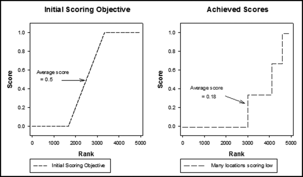
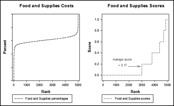
Equation (16.11) for P2 has a few interesting properties. The fraction within the cubed root sign will always be in the 0 to 1 range, which is what we want for the risk-scoring systems. Taking the cubed root keeps the calculated value in the 0 to 1 range but it has the effect of scoring low proportions with a higher P2 score. For example, the cubed root of 0.1 is 0.464, the cubed root of 0.2 is 0.584, and the cubed root of 0.3 is 0.669. The average cash tickets proportion was about 0.125 and so the agencies would on average score 0.50 for P2. The scoring objective in this application was to score the average agency at 0.50. That objective has since changed to score the average forensic unit at about 0.05 to 0.20 for each predictor.
P3: Void Count above Average
This predictor looked at whether the count of voids for the immediately past week was high when compared to the count of voids for the prior four weeks. A nonlinear function was used and the equation is shown in Equation (16.12).
(16.12) 
The cubed root in Equation (16.12) transforms a proportion of 0.25 to 0.63. If all weeks had an equal void count, the count for one week should be about one-quarter of the total count. With the cubed root the average agent would score 0.66 for P3. With hindsight it would seem that this predictor was not properly scored. A scoring formula that was based on the distance above 0.25 would have been more appropriate. Such a scoring formula is shown in Equation (16.13).
(16.13) 
where VP is the void proportion for the count of voids this week divided by the count of voids for the past four weeks.
The scoring formula in Equation (16.13) would score a void proportion of 0.26 (slightly higher than one-quarter) as 0.10, and a void proportion of 0.35 (much higher than one-quarter) as 1.00 indicating a high risk for the fraud scheme.
P4: International Ticket Proportion
The fraud scheme was focused on tickets to international destinations because foreign ticket prices are higher than normal, the flight date is usually further into the future, and the passenger is more likely to pay by cash or check. A high proportion of international tickets would suggest that the agency is a high-risk agency. The formula used to score P4 is shown in Equation (16.14).
(16.14) 
Equation (16.14) uses the cubed root, which has the effect of giving the average agency a P5 score of about 0.50 because foreign sales were usually about 12 percent of total sales. More recent applications of risk scoring would use a scoring formula that assigns a lower score to the average forensic unit.
P5: High-Risk States
The target victims of the scheme were immigrants wanting to fly home on a bargain airfare. The fraudsters would therefore try to carry out a void fraud scheme from a location with many immigrants in the vicinity. P5 identified those states with (a) large immigrant populations, and (b) a history of such schemes being carried out or attempted. The result was that forensic units located in certain high-risk states were scored as high-risk for P5. The scoring formula is shown in Equation (16.15).
(16.15) 
P5 uses an indicator variable with a score of 0 or 1. The indicator can work both ways. Forensic units can be scored with a 1 if they meet certain criteria and a 0 otherwise. Alternatively, forensic units can be scored with a 0 if they meet certain criteria and a 1 otherwise. The IRS might score certain taxpayers as 0 if it believes the taxpayers to be fully compliant. A reason for such a belief might be that the taxpayer has been audited more than once with no increases in taxes owed.
P6: Dollars at Risk
For P6 a forensic unit was given a high score if the sum of the cash voids for the prior week was high. The logic is that the more voids that are occurring, the higher the risk for the forensic unit. If there was only a small level of void activity measured by total dollars, the risk attached to that forensic unit would be small. Using the analysis of the average void activity, the scoring formula in Equation (16.16) was developed.
(16.16) 
where VS is the Void Sum for the prior week.
The effect of using logs is that a forensic unit will be given a reasonably high score for a void sum that is not too much higher than $5,000. For example, a void sum of $10,000 will be given a P6 score of 0.301. A void sum of $15,000 will be given a P6 score of 0.477. The increase in P6 is at an ever-decreasing rate. At or above $50,000, the score will be 1.00. This predictor was seen to be very important and it ended up with the highest weight for any predictor.
P7: Nonreporting
This predictor looked at whether the forensic unit was guilty of any tardy behavior that might be a predictor that some or other scheme was in the works. This is similar to the belief in law enforcement that citizens who have a general contempt for the law will probably be breaking many different laws. This is why someone pulled over for speeding (a specific law) is given some general questioning and perhaps a search because the speeding offense could be a signal that the person has a contempt for law and order in general. For example, on April 19, 1995, Timothy McVeigh was stopped by a state trooper for driving without a license plate.
If a passenger arrives at the airport and the ticket sale was not reported to the carrier, this was a sign of tardy records and procedures. In this case a forensic unit was given a score of 1.00 if there were any unreported sales, and a score of 0 otherwise. These unreported sales were rare and P7 was given a relatively low weighting.
P8: Carrier Void Concentration
The P8 predictor gave a high score to forensic units that had most of their voids concentrated on one or two carriers only as opposed to having their voids spread across many carriers. It was a trademark of the scheme that specials were offered for one or two destinations and many tickets were sold for that overseas route. The scoring formula is shown in Equation (16.17).
(16.17) 
The scoring formula in Equation (16.17) turned a fraction with a low proportion (one carrier and 10 voids, which gives one-tenth for the fractional part) into a high score (of 0.95). Some examples of P8 scores are shown below:
1 carrier and 10 voids: P8 score of 0.95
1 carrier and 25 voids: P8 score of 0.98
5 carriers and 10 voids: P8 score of 0.71
5 carriers and 50 voids: P8 score of 0.95
P8 will give high scores for many voids and fewer carriers. After the addition of P8 to the list of predictors, the scoring system was thought to have enough predictive capability.
Final Results
The predictors were weighted for the final risk scores. This was a complex process and involved many iterations. The weighting method used five successful cases of the fraud. The data was then analyzed for the week in which it was felt that the fraud was well underway (usually the second week of the fraud). The analysis showed where that forensic unit was ranked in the rankings. The weightings were continually revised until the fraudulent agent was in the top 50 high-risk agents. The process went through many iterations with different weightings until the highest possible score across all five known past fraud cases was achieved.
Table 16.2 The Weightings of the Airline Fraud Predictors.
| P1, Average void amount |
0.100 |
| P2, Cash ticket proportion |
0.100 |
| P3, Void count above average |
0.150 |
| P4, International ticket proportion |
0.150 |
| P5, High-risk states |
0.125 |
| P6, Dollars at risk |
0.200 |
| P7, Nonreporting |
0.075 |
| P8, Carrier void concentration |
0.100 |
| Sum of Weights |
1.000 |
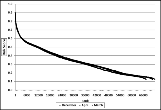
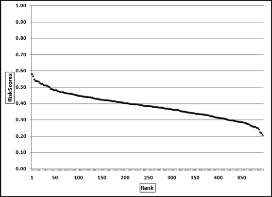
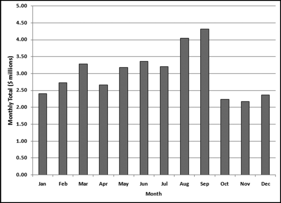
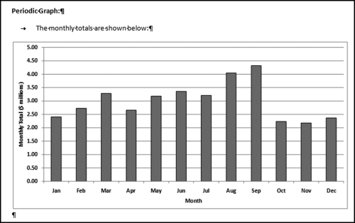
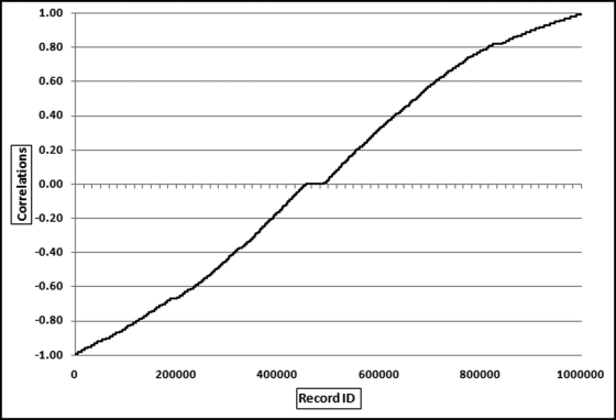
Table 16.2 shows the predictors and their weights. The final objective was to identify the high-risk cases and to end up with scores where there were only a few high scores. Another consideration was that the distribution was somewhat stable from week to week. It seems logical that a risk-scoring system should generate scores that have similar patterns from week to week. The risk scores were calculated for three dates and the graph is shown in Figure 16.1.
Figure 16.1 shows that the pattern of the risk scores is very similar for the three dates selected. The results also show that there is only a small group of forensic units with high scores. In this case a high score seems to be a score of 0.70 and higher. The final reports used by the forensic investigators included some details relevant to the scoring procedure, such as average void in dollars, the number of voided carriers, and the total void percentage. The project was a success.
Risk Scoring to Detect Vendor Fraud
In 2009 this project was discussed with the auditors of an international conglomerate. The goal of the risk-scoring method was to detect vendor fraud. The project was given to an auditor but the system was never developed because it was just too difficult to get invoice-by-invoice data. Payments data was available as a part of a system to test for duplicate payments, but payments data (checks and wire transfers paid to vendors) could aggregate several invoices and payments data does not directly show credits. An invoice for $20,000 and a credit of $3,000 would end up as a single payment of $17,000. The details of the credit would be lost. The invoice data resided in too many different systems and was also simply too large (in terms of gigabytes) to download and analyze in Access. The formulas that would have been used are discussed below together with Access queries applied to the invoices data from Chapter 4. The predictor variables are discussed next.
P1: Invoice Count
The position was taken that a fraudulent vendor would not have too many invoices per month. Each invoice creates a risk for the fraudster and the belief was that they would try to at least keep that risk reasonable. The P1 scoring formula is a 0/1 indicator variable that scores a 0 if the vendor has more than six invoices in any single month and a 1 otherwise. This is set out in Equation (16.18).
(16.18) 
The scoring formula in Equation (16.18) would be quite easy to program in Access. If data from more than one year is being used, the equation could be changed to an invoice count of less than or equal to eight invoices to take account of the fact that the fraudster might occasionally deviate from the norm.
P2: Credits, Adjustments, and Reversals
The position was taken that a fraudulent vendor would not have any credits, adjustments, or reversals since no goods or services were actually provided. The fraudster would presumably try to have the invoice glide through the payments process with the absolute minimum of fanfare. Nigrini (1999) reviews an interesting case of vendor fraud, State of Arizona v. Wayne James Nelson (CV92-18841), where Nelson was found guilty of trying to defraud the state of $2 million. Nelson, a manager in the office of the Arizona State Treasurer, claimed that he had diverted funds to a bogus vendor to show the absence of safeguards in a new computer system. The amounts of the 23 checks are shown in Table 16.3.
Table 16.3 The Checks that a Treasurer for the State of Arizona Wrote to a Fictitious Vendor.
| October 9 |
1,927.48 |
|
27,902.31 |
| October 14 |
86,241.90 |
|
72,117.46 |
|
81,321.75 |
|
97,473.96 |
| October 19 |
93,249.11 |
|
89,658.17 |
|
87,776.89 |
|
92,105.83 |
|
79,949.16 |
|
87,602.93 |
|
96,879.27 |
|
91,806.47 |
|
84,991.67 |
|
90,831.83 |
|
93,766.67 |
|
88,338.72 |
|
94,639.49 |
|
83,709.28 |
|
96,412.21 |
|
88,432.86 |
|
71,552.16 |
| Total |
1,878,687.58 |
No services were ever delivered, so Nelson must have invented all the numbers in his scheme, and because people are not random, invented numbers are unlikely to follow Benford's Law. There are several indications that the data is made up of invented numbers. First, he started small and then increased the dollar amounts. The jumps were large, at least to the threshold of $100,000. Most of the dollar amounts were just below $100,000. It is possible that $100,000-plus amounts would receive additional scrutiny or that checks above that amount required human signatures instead of automated check writing. The digit patterns of the check amounts are almost opposite to those of Benford's Law. More than 90 percent of the amounts have a high first digit. Had each vendor been tested against Benford's Law, this set of numbers also would have had a low conformity to Benford as measured by the MAD.
The numbers seem to have been chosen to give the appearance of randomness. None of the check amounts were duplicated; there were no round numbers; and all the amounts included cents. Subconsciously though, the manager repeated some digits and digit combinations. Among the first-two digits of the invented amounts, 87, 88, 93, and 96 were all used twice. For the last-two digits, 16, 67, and 83 were duplicated. There was a general tendency toward the higher digits with 7 through 9 being the most frequently used digits. A total of 160 digits were used in the 23 numbers. The counts for the 10 digits from 0 to 9 were 7, 19, 16, 14, 12, 5, 17, 22, 22, and 26, respectively. An investigator familiar with Benford's Law would have seen that these numbers—invented to seem random by someone ignorant of Benford's Law—fall outside of the expected patterns and so merit a closer investigation.
Although the Arizona case violates the P1 predictor (there are more than six invoices), there are no credits and so the vendor would score a 1 on P2. The idea behind using multiple predictors is that no single predictor is, by itself, a perfect indicator. The P2 scoring formula is a 0/1 indicator that scores 0 if the vendor has any credits, adjustments, or reversals for the period under review and a 1 otherwise. This is set out in Equation (16.19).
(16.19) 
The scoring formula in Equation (16.19) would be quite easy to program in Access. Note that P1 and P2 are similar in that P1 scores 1 when the count is “low” (less than or equal to 6) and P2 also scores 1 when the count is “low” (zero). A low count of invoices and a low count of credits, adjustments, or reversals raise the risk of the vendor being fraudulent.
P3: Increase in Dollars over Time
A common theme in most frauds is that the fraudsters just do not know when to stop. The case of a large metropolitan housing authority that used an off-duty policeman to patrol its housing units is reviewed in Nigrini (1994). From 1981 to 1991 the head of security managed to embezzle about $500,000 by submitting phony time records and pay claims for work done by police officers. The policeman named on each timesheet were real people who worked for the authority, but the purported work done and hours worked were phony.
Each payday the security chief would go to the bank to cash checks for policemen who had worked, but were now back on regular duties in the city. There were usually one or two checks drawn for work done that were cashed and the cash kept by the security chief for his own use.
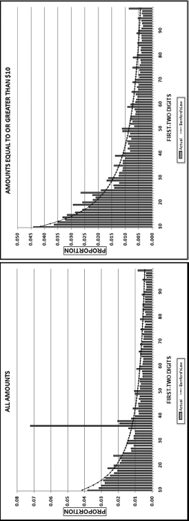
The security chief had to invent a fictitious work schedule, so the dollar amounts of the fraudulent checks lent themselves to an interesting application of Benford's Law. The time period of the fraud was divided into two five-year periods. Benford tests were designed to also see whether the security chief's number invention patterns changed over time or whether he was consistent over time.
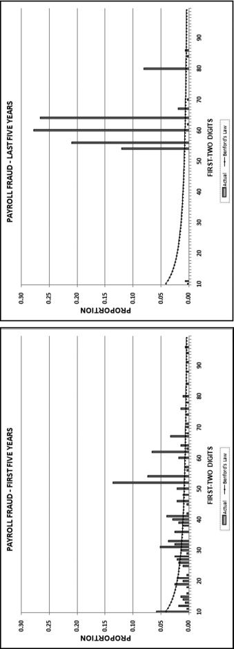
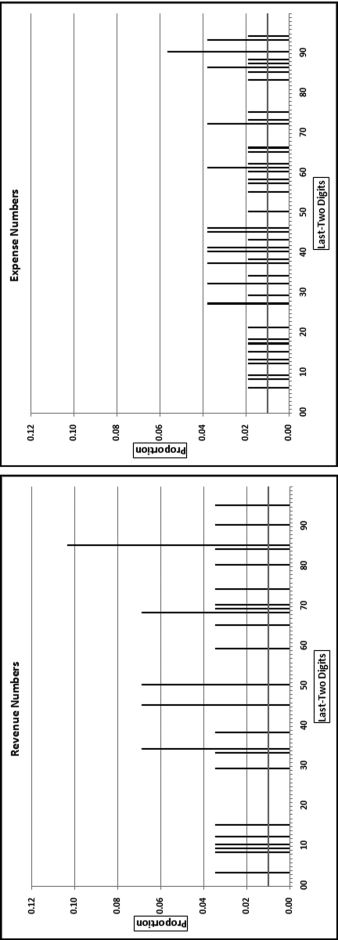
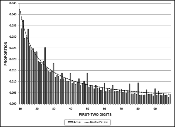
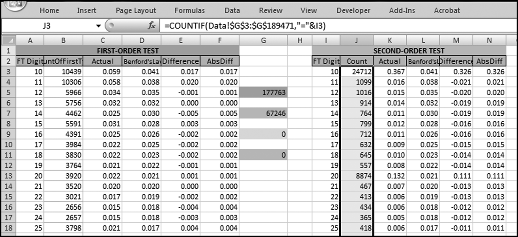
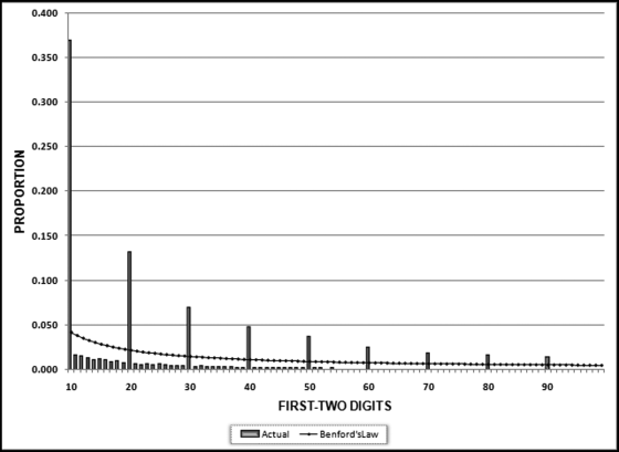
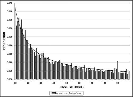
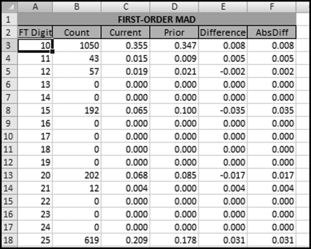
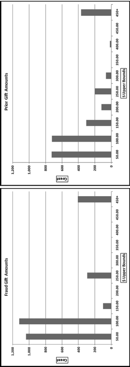
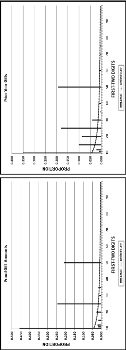
The first-order test of the 273 fraudulent checks for the first five years of the fraud (1981 to mid-1986) is shown in the left panel of Figure 16.2. Some large positive spikes are evident and many different combinations were used. The fraudster used 52 of the possible 90 first-two digit combinations. The most frequently used numbers were $520, $540, $624, $312, $416, and $100. The check amounts ranged from $50 to $1,352 and totaled approximately $125,000. In the Arizona fraud case Nelson started off small and then quickly increased the fraudulent check amounts. This was also the case here in that the dollar amount tripled in the last five years.
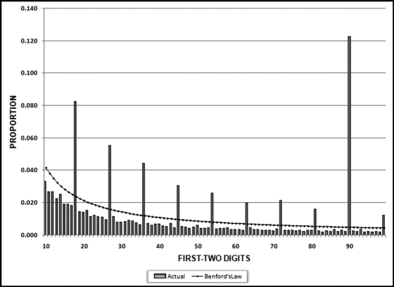
The first-two digits of the 600 fraudulent checks for the last five years of the fraud (mid-1986 to 1991) are shown in the right panel of Figure 16.2. There are fewer significant spikes, and the significant spikes are larger. The MAD is larger for the right-hand side graph (the numbers for the last five years). Only 14 of the possible 90 first-two digit combinations were used, indicating that the security chief was gravitating toward using the same numbers over and over again. The most frequently used numbers were $600, $640, $560, $540, and $800. The check amounts ranged from $540 (much higher than the previous lows) to $1,120 and totaled approximately $375,000.
It is interesting that as time passed so the security chief gravitated toward reusing the same set of numbers. Over time the quantity and the amounts increased. The security chief used the names of valid policemen. An audit would have shown that the policemen often worked 40-hour weeks, yet there were no arrest or activity records for the energetic policemen working two full-time physically demanding jobs for that week. Given the size of the spikes on the 1986–1991 graph it is almost certain that these digit combinations would have spiked during an analysis of the general disbursements account (the account from which the policemen were paid).
This fraud would still be in progress had it not been that one Friday the security chief entered the bank to cash his usual package of checks. The teller happened to know one of the “prior-week” policemen whose check was cashed and who happened to be on-duty in the bank at the time. Later that afternoon she told the policeman that “security chief” had cashed his check and would probably have the cash at the station on Central Parkway soon. He was rather surprised by her statement because he had spent his off time that week working in the bank. The security chief was probably more surprised when he was arrested (probably not by the bank policeman) but none were as surprised as the management of the bank, which was sued for $100,000 for negligence by the housing authority. Using the fact that the fraud tripled in the past five years, an example of a scoring formula would be as shown in Equation (16.20).
(16.20) 
where Increase is calculated as [(Current period)/(Prior period)] −1.00. A total for the current period of $6,000 and a total for the prior period of $4,000 would give an Increase of 0.50. Using the scoring formula in Equation (16.20), an increase of 0.50 would be scored with a P3 score of 0.625.
P4: Dollar Amounts
Another common theme in most frauds is that fraudsters do not just steal a small number of dollars, they tend to go so high that one is forced to wonder what they were thinking. This was definitely the case with the Charlene Corley fraud discussed in Chapter 3. The general rule is that no fraudster gets away with (say) $3,000 and then stops. P4 is there to keep forensic investigators focused on the large dollars, and vendors that are in the usual fraud range. Except for Charlene Corley, frauds are unlikely to be very large amounts. The scoring formula in Equation (16.21) discards vendors that are too small and also those that are too large.
(16.21) 
Where Total is the total dollars invoiced by the vendor over the past year. Ideally this equation should have a rapid increase to 1.00 (at a dollar value of $50,000) and then a gradual decrease to zero at $500,000. Such a formula would be too complex for this example.
P5: Round Number Dollars
A belief is that fraudsters use round numbers because these are easier to keep track of. Several years ago a Texas-based divisional controller believed that he was too busy to approve all the invoices for payment. He asked his administrative assistant whether she would approve all invoices under $5,000 for payment. She replied that she was happy to do this. Her fraud was detected about $500,000 later. The forensic investigation showed that almost all of the invoices were for round numbers (multiples of $100) that were less than $5,000. Some of the invoices were very primitive being, for example, an invoice for $2,800 for “office party.” A possible scoring formula is shown in Equation (16.22).
(16.22) 
The square root has the effect of giving reasonably high scores to small round proportions. For example, a round proportion of 0.30 (perhaps 6 of 20 invoices are round) would be given a P5 score of 0.548.
P6–P14: Other Predictors
The predictors discussed in P1–P5 would be a good starting point. There are other possible predictors that could also be used and the logic would remain the same. Situations that are high risk would be scored as 1.00 and low-risk situations would be scored as 0.00. Each of these predictors would have a scoring formula and a weight in the final score. Examples of additional predictors are:
- Vendor's invoices are predominantly for services as opposed to goods for resale or for a production process.
- Vendor has invoices without purchase orders.
- Vendor has a regular pattern of invoices (e.g., one every week or two every month).
- Vendor has higher purchases just before Christmas holidays.
- Vendor's tax ID is a social security number.
- Vendor has excessive invoices just below key approval amounts or psychological thresholds.
- Vendor has many invoices dated on weekends or public holidays, or seems to favor one day of the week for invoicing.
- Vendor is consistently paid quickly or is paid in some way that is abnormal for the company.
- Vendor has a history of changes to the vendor master record (bank account changes or address changes).
The predictors listed above are not included in the Access demonstration in the next section. Access works well unless the number of forensic units is very large or there are many predictors with complex calculations.
Vendor Risk Scoring Using Access
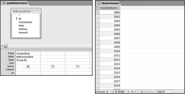
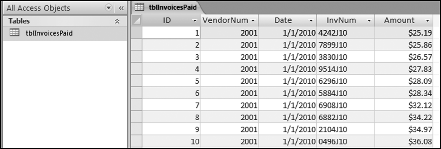
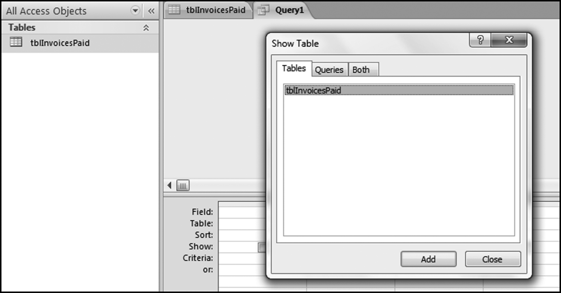
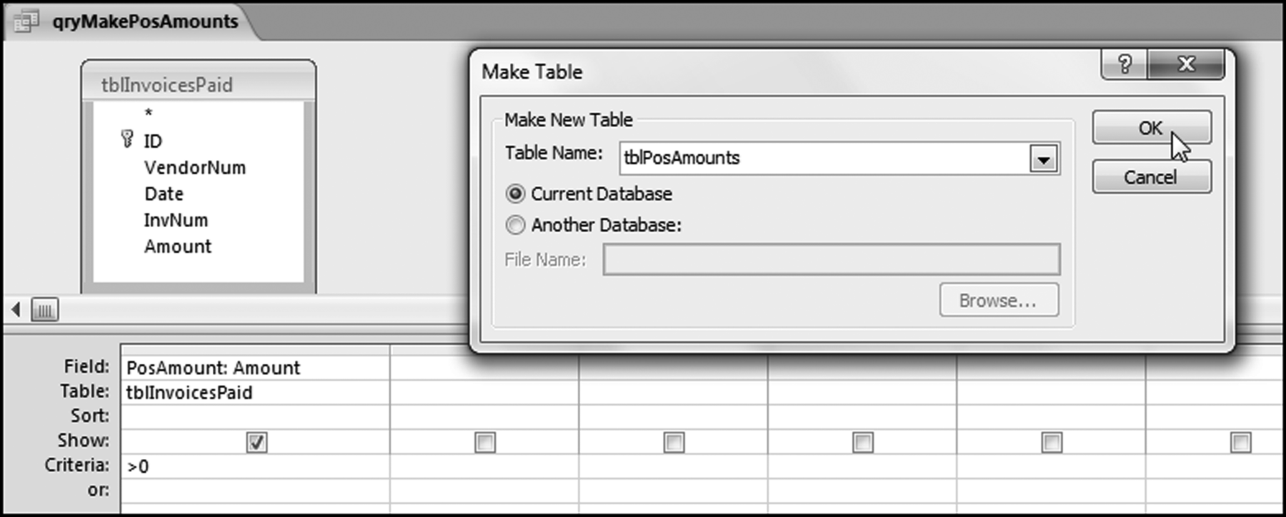
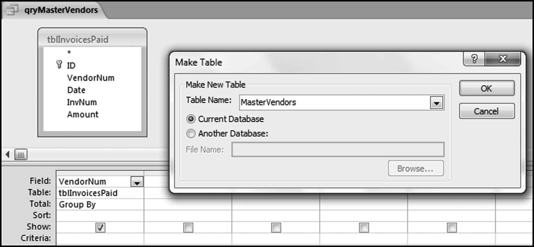
The risk-scoring method will be applied to the Invoices data from Chapter 4. The first step in the analysis is to create a table listing all the vendors that should be scored. This table will ensure that we have a score for each forensic unit and no null scores when it comes to calculating the final score. The make-table query and the results are shown in Figure 16.3.
This table should be used in any query when it is possible that the results do not end up with a score for all 26,166 vendors and it is necessary to force a score of 0 or 1 for the missing vendors. This will become clearer when the P3 queries are shown.
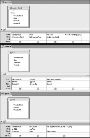
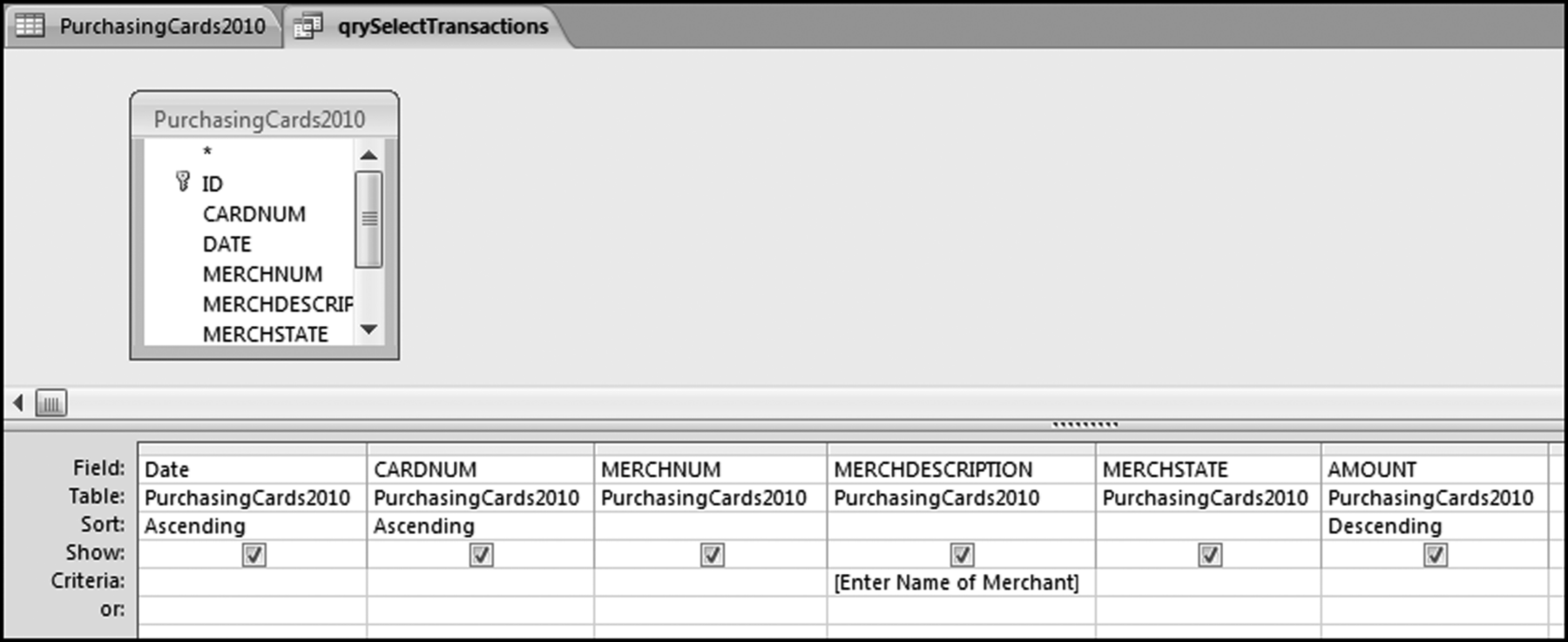
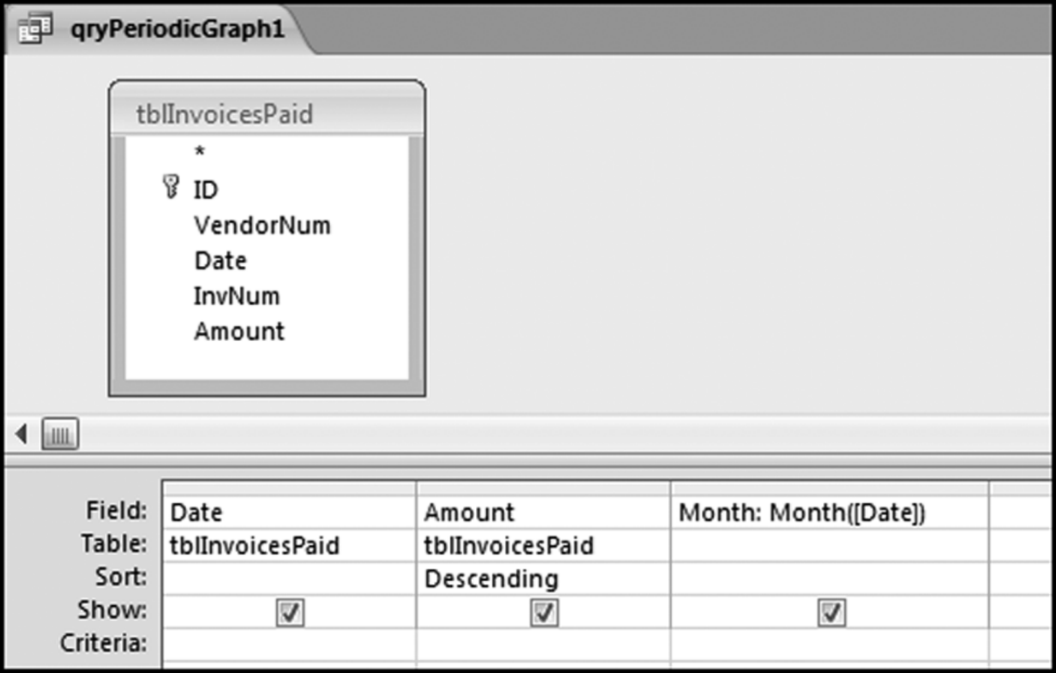
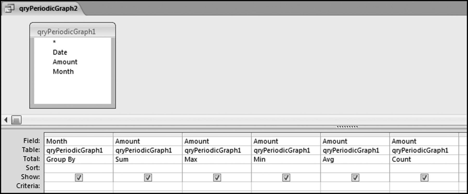
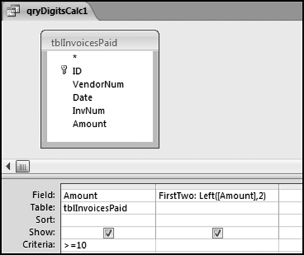
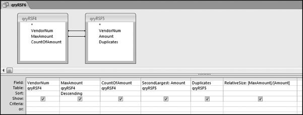
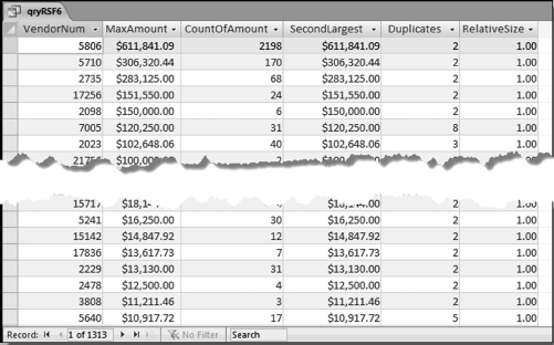
The query to score P1 is shown in Figure 16.4. A series of three queries is needed. The first query calculates the invoice month using the MONTH function. The second query counts the number of invoices for every month that the vendor actually has any invoice. The third query calculates the maximum for any month for each vendor. The third query also scores the vendor using the formula in Equation (16.18).
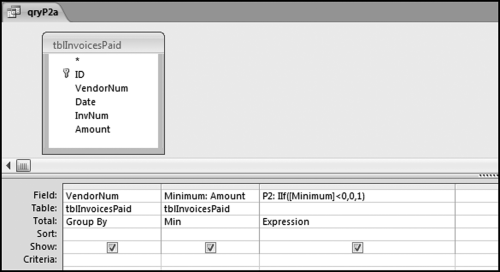
The series of queries for P1 is shown in Figure 16.4. The vendor is scored with a zero if the count in any month exceeds five invoices. The query used to score P2 is shown in Figure 16.5. The logic used is that if the minimum amount is less than zero then the vendor has a credit, adjustment, or reversal of some sort. The predictor P2 is then scored using the IIF function.
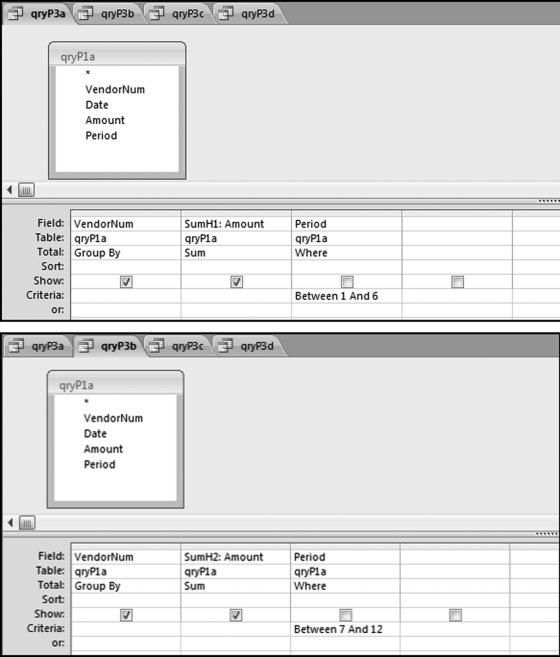
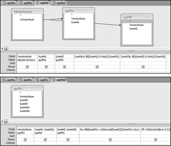
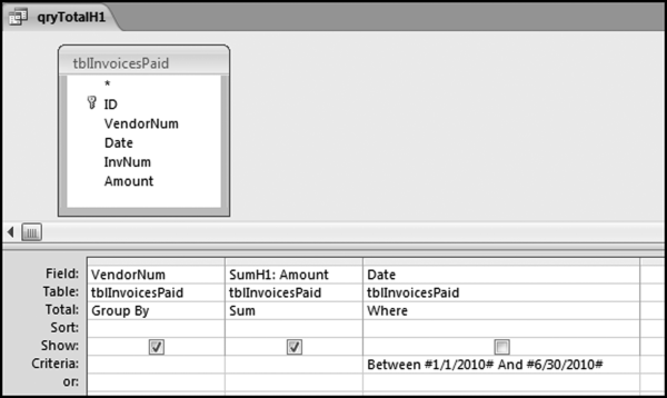
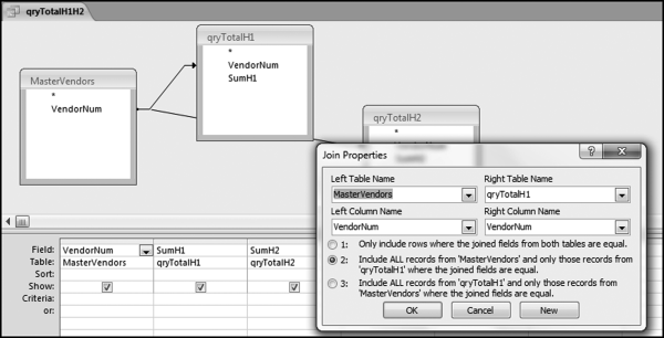
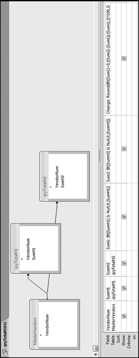
If the vendor has any amount less than zero then the vendor is scored with a zero. The series of queries needed to score P3 compares the total dollars for the last six months of the year (H2) with the total dollars for the first six months of the year (H1). It would seem that this would be an easy predictor to program. The issues arise when a vendor has transactions in either H1 or H2, but not in both periods. This makes the sum for H1 or H2 a null value rather than zero. The solution is to convert the null values to zeroes. The set of queries used to calculate the H1 and H2 sums are shown in Figure 16.6. The set of queries used to score P3 is shown in Figure 16.7.
The queries used to calculate the H1 and H2 sums uses the Between function in the Criteria. The Between function includes both of the numbers used in the Between statement. The query used for the comparisons and to score P3 is shown in Figure 16.7.
Figure 16.7 shows qryP3c, which is the query used to convert null values to zeroes. The use of the MasterVendors table makes sure that there is one record for each vendor. The query also changes the null values to zeroes with the following IIF functions and the Is Null criteria:
SumH1b: IIf([SumH1] Is Null,0,[SumH1])
SumH2b: IIf([SumH2] Is Null,0,[SumH2])
The final query to score P3 renames the SumH1b and SumH2b fields back to SumH1 and SumH2. The increase from H1 to H2 is calculated using the following calculated field:
Inc: IIf([SumH1]<>0,Round([SumH2]/[SumH1]-1,4),1)
The IIF function is used to calculate the increase from H1 to H2 to make sure that there is never a division by zero error. The last formula applies Equation 16.20 and is shown below:
P3: Val(Switch([Inc]<0.2,0,[Inc]<1,Round(([Inc]-0.2)∗1.25,4),[Inc]>=1,1))
The P3 formula uses the SWITCH function in Access, which allows for multiple IIF criteria. The function applies the first true criterion when moving from left to right in the function. The results of the SWITCH function are shown as text and the use of VAL changes the text format to a numeric result. The ROUND function keeps the results neat.
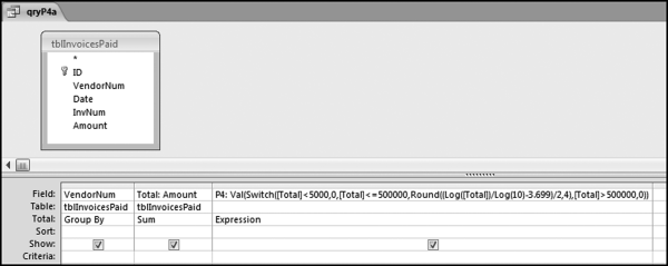
The query used to score P4 is shown in Figure 16.8 with the SWITCH function and the VAL function used to convert the text values to numeric values. The formula used is
P4: Val(Switch([Total]<5000,0,[Total]<=500000,Round((Log([Total])/Log(10)-3.699)/2,4),[Total]>500000,0))
The division by log(10) is there because Access calculates the natural log (base e) of a number using the LOG function. The division by log(10) converts the natural log (usually written as ln) to the log to the base 10. The queries used to score P5 are shown in Figure 16.9.
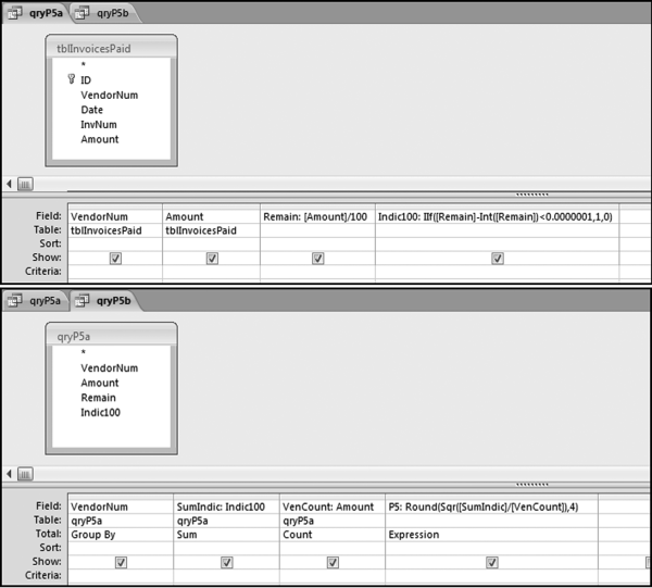
The first query calculates whether a number is round (neatly divisible by 100). The formulas used in query qryP5a are
Remain: [Amount]/100
Indic100: IIf([Remain]–Int([Remain])<0.0000001,1,0)
A mathematically perfect formula would use an equals sign (=) instead of the less than (<) sign. The less than sign (<) is preferred because it takes account of possible problems with the limited precision of personal computers.
The formula used to score P5 in qryP5b uses the square root SQR function and also the ROUND function to keep the results tidy and is set out below:
P5: Round(Sqr([SumIndic]/[VenCount]),4)
The final step in the risk-scoring system is to calculate a final risk score for all vendors. The weightings used are shown in Table 16.4.
Table 16.4 The Weightings Applied to the Fraud Risk Predictors.
| P1, Invoice count, not too large |
0.15 |
| P2, No credits, adjustments, or reversals |
0.15 |
| P3, Increase in dollars |
0.40 |
| P4, Total dollars, not small and not large |
0.20 |
| P5, Round numbers |
0.10 |
| Sum of Weights |
1.00 |
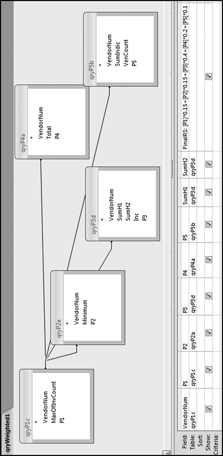
The largest weight is given to the increase in dollars. The lowest weight is given to the round number predictor. The query used to calculate the risk score is shown in Figure 16.10.
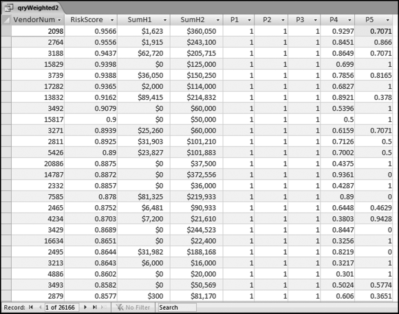
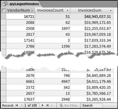
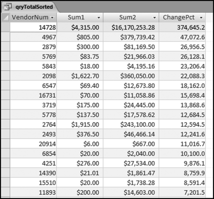
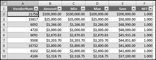
The final risk score is calculated in Figure 16.10. The risk score is simply the sum of the P-scores multiplied by their weights. The fields SumH1 and SumH2 are added to the query grid for informational purposes. For large files or for more predictors this query might not execute quickly. The solution is to create temporary tables (using make-table queries) of the predictors that require the most processing capacity (in this case it would be P3). The final step (not shown) is to sort the risk scores descending with a new query that only sorts FinalRS descending. The new query would also round FinalRS to four places after the decimal point and would rename the field RiskScore. The query would also show SumH1 and SumH2 in whole dollars only. This query was named qryWeighted2 and the results are shown in Figure 16.11.
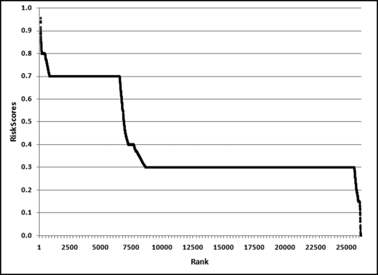
The results in Figure 16.11 show that there are several vendors with very high scores. This means that these vendors “satisfied” almost every category of risk scoring. A graph of the risk scores sorted descending is shown in Figure 16.12.
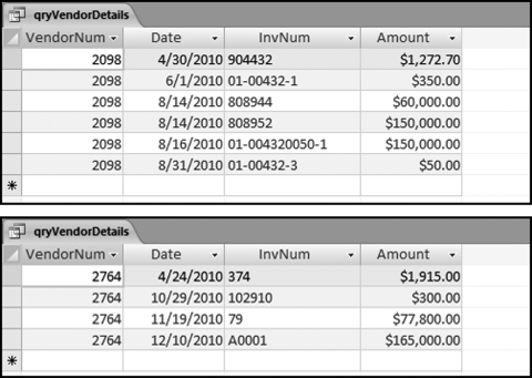
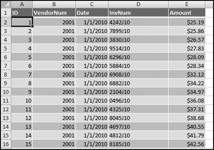
The risk-scoring results show a small slice of high-scoring forensic units. In this case 91 vendors (0.3 percent) have risk scores that are greater than 0.80 and 366 vendors have risk scores that are equal to 0.80. The transactions of the two highest scoring vendors are shown in Figure 16.13.
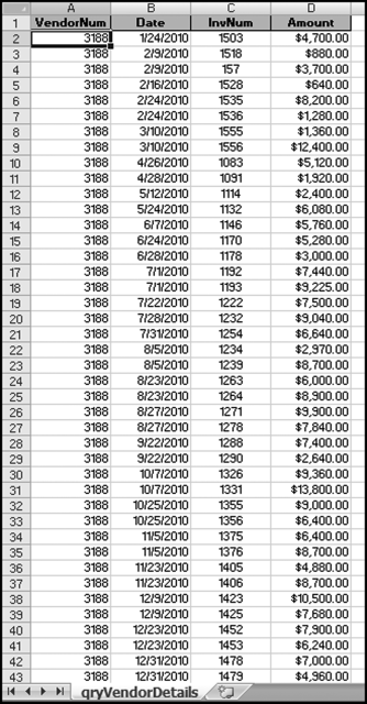
The numbers in Figure 16.13 confirm that the risk-scoring system is calculating correctly. The H2 totals are significantly more than the H1 totals. There are no credits and the count for every month is six or fewer invoices. Many of the numbers are round and the totals are both above $250,000 but less than $500,000. A problem with the risk-scoring formula is that we seem to have one-third of the invoices being for more than $100,000. In accounts payable settings invoices for $100,000 or more are thoroughly audited before payment is made, even when the accounts payable function is outsourced. It would seem that refinements to the risk-scoring formulas could include a predictor that scores high if all invoices are less than $50,000, approximately 0.50 if some invoices are in the $50,000 to $100,000 range, and low if many invoices exceed $100,000 (as is the case in Figure 16.13). The third highest scoring vendor (vendor #3188 with a risk score of 0.9437) shows another interesting pattern of invoices. The transactions are shown in Figure 16.14.
The transactions for vendor #3188 warrant a closer look. The vendor has the right number of invoices (about four per month), there are no credits, there is a growth over time, many of the numbers are round, and the total is just about right at $270,000 per year. In addition, there are no “large” invoices (over $50,000). The investigation is made much easier if the images of the invoices are accessible.
Summary
The chapter reviewed the audit selection method of the Internal Revenue Service (IRS). The IRS scoring method analyzes the differences between those tax returns with an insignificant tax change and those tax returns with a significant tax due change. The analysis is based on an intensive audit of thousands of taxpayers. Discriminant analysis is used to distinguish between the two taxpayer groups. Returns are scored as to whether they more closely resemble the no change group or the significant tax due change group. The method results in a DIF (Discriminant Index Function) score for each taxpayer. Both the risk-scoring and the DIF methods seek to score forensic units so that audit efforts are directed toward high-risk forensic units. Both methods use predictor variables, although the taxpayer predictors are “chosen” by the discriminant model, and in the risk-scoring method the predictors are chosen by industry experts. Both methods require regular updates and changes to the selection formulas.
A risk-scoring application for banking fraud was reviewed. Check kiting occurs when a bank account holder successfully withdraws funds from an account where the funds are made up of uncollected funds. The system was designed to rank bank accounts in terms of their check-kiting risk so that the bank investigators could focus their energies and efforts on the high-risk candidates. The system used seven predictors and the most important predictors were frequent deposits from the same routing number, drawing on uncollected funds, and recent returned (bounced) deposits.
A risk-scoring application to detect a type of travel agent fraud was reviewed. Agents sold airline tickets and then voided the tickets in the reservation system and pocketed the cash. The risk-scoring system used predictors such as the average voided amount, excessive voids in the current week, international sales, location of the forensic unit, and whether the voids were being carried out against just one or two carriers. This system was programmed on a mainframe computer. The system was judged a success by management and by the auditors.
A risk-scoring system to detect fictitious vendors was also reviewed. The predictors looked for vendors that were not too big and not too small, vendors that had no credits, adjustments, or reversals, vendors that showed an increase over time, and vendors with round dollar amounts. The equations were reviewed as well as the Access queries used to implement the risk scoring system. Access can calculate the final weighted scores as long as there are not too many forensic units or queries, and as long as there are no calculation errors (perhaps because of division by zero). The results showed a small group (0.3 percent) of high-risk vendors.





















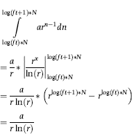
 (2/1000)” term is



 or some smaller root to take account of the practical issues encountered with real world data sets.















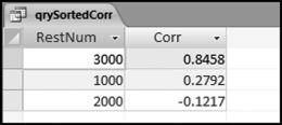
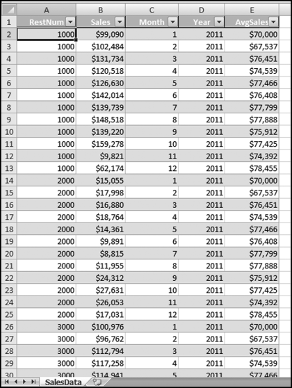
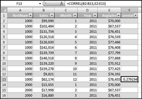
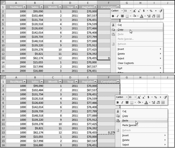






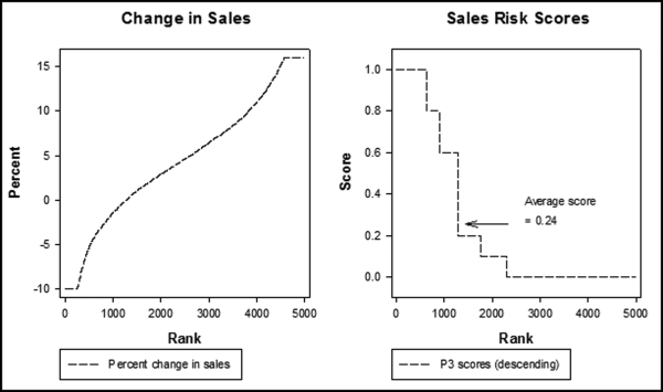
 representing the change in Sales.

 are the optimal weights, and the
  are the predictors.


