
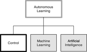
Pattern recognition in images is a classic application of neural nets. This chapter builds upon the previous one by exploring multi-layer networks, which fall into the Machine Learning branch of our Autonomous Learning taxonomy. In this case, we will look at images of computer-generated digits, and the problem of identifying the digits correctly. These images will represent numbers from scanned documents. Attempting to capture the variation in digits with algorithmic rules, considering fonts and other factors, quickly becomes impossibly complex, but with a large number of examples, a neural net can readily perform the task. We allow the weights in the net to perform the job of inferring rules about how each digit may be shaped, rather than codifying them explicitly.
For the purposes of this chapter, we will limit ourselves to images of a single digit. The process of segmenting a series of digits into individual images is one that may be solved by many techniques, not just neural nets.
9.1 Generate Test Images with Defects
9.1.1 Problem
The first step in creating our classification system is to generate sample data. In this case, we want to load in images of numbers for 0 to 9 and generate test images with defects. For our purposes, defects will be introduced with simple Poisson or shot noise (a random number with a standard deviation of the square root of the pixel values).
9.1.2 Solution
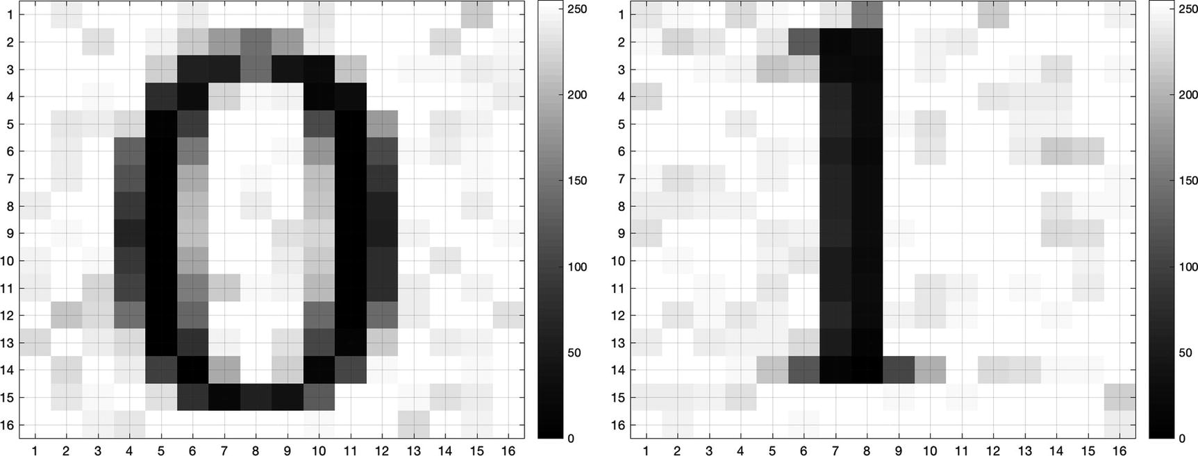
A sample image of the digits 0 and 1 with noise added.
9.1.3 How It Works
The code listing for the CreateDigitImage function is below. The inputs are the digit and the desired font. It creates a 16x16 pixel image of a single digit. The intermediate figure used to display the digit text is invisible. We will use the ’RGBImage’ option for print to get the pixel values without creating an image file. The function has options for a built-in demo that will create pixels for the digit 0 and display the image in a figure if no inputs or outputs are given. The default font if none is given is Courier.
TIP
Note that we check that the font exists using listfonts before trying to use it, and throw an error if it’s not found.
Now, we can create the training data using images generated with our new function. In the recipes below we will use data for both a single-digit identification and a multiple-digit identification net. We use a for loop to create a set of images and save them to a MAT-file using the helper function SaveTS. This saves the training sets with their input and output, and indices for training and testing, in a special structure format. Note that we scale the pixel values, which are nominally integers with a value from 0 to 255, to have values between 0 and 1.
Our data generating script DigitTrainingData uses a for loop to create a set of noisy images for each desired digit (between 0 and 9). It saves the data along with indices for data to use for training. The pixel output of the images is scaled from 0 (black) to 1 (white), so it is suitable for neuron activation in the neural net. It has two flags at the top, one for a one-digit mode and a second to automatically change fonts.
The helper function will ask for a filename and save the training set. You can load it at the command line to verify the fields. Here’s an example with the training and testing sets truncated:
Digit Training Sets
’Digit0TrainingTS’ | Single-digit set with 120 images of the digits 0 through 5, all in the same font |
|---|---|
’Digit0FontsTS’ | Single-digit set of 0 through 5 with random fonts |
’DigitTrainingTS’ | Multi-digit set with 200 images of the digits 0 through 9, same font |
We have created the following sets for use in these recipes:
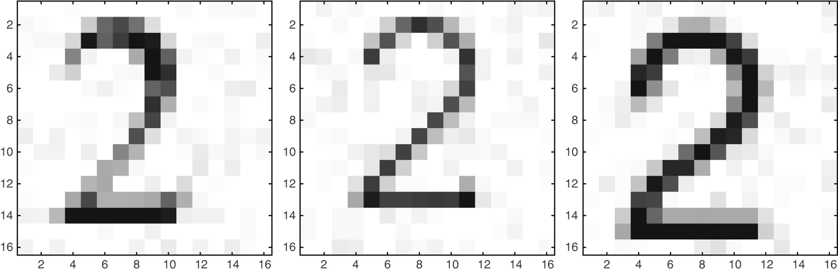
Images of the digit 2 in different fonts.
9.2 Create the Neural Net Functions
9.2.1 Problem
We want to create a neural net tool that can be trained to identify the digits. In this recipe we will discuss the functions underlying the NeuralNetDeveloper tool, shown in the next recipe. This interface does not use the latest graphic user interface (GUI)-building features of MATLAB, so we will not get into detail about the GUI code itself although the full GUI is available in the companion code.
9.2.2 Solution
The GUI uses a multi-layer feed-forward (MLFF) neural network function to classify digits. In this type of network, each neuron depends only on the inputs it receives from the previous layer. We will discuss the function that implements the neuron.
9.2.3 How It Works
The basis of the neural net is the Neuron function. Our neuron function provides six different activation types: sign, sigmoid mag, step, logistic, tanh, and sum [22]. This can be seen in Figure 9.3.
 . Two other functions useful in multi-layer networks are exponential (sigmoid logistic function):

It is a good idea to try different activation functions for any new problem. The activation function is what distinguishes a neural network, and machine learning, from curve fitting. The input x would be the sum of all inputs plus a bias.
TIP
The sum activation function is linear and the output is just the sum of the inputs.
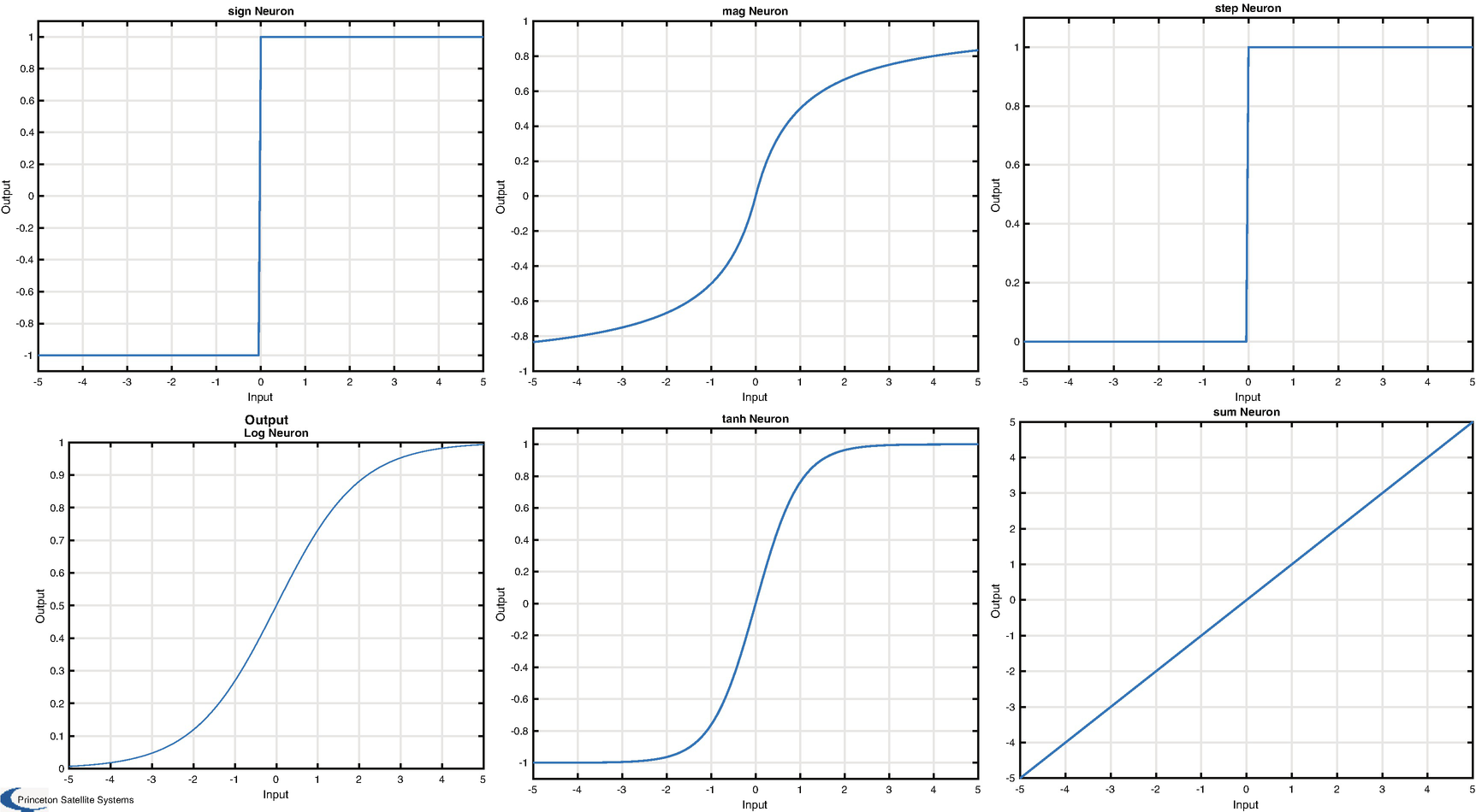
Available neuron activation functions: sign, sigmoid mag, step, logistic (log), tanh, and sum.
Neurons are combined into the feed-forward neural network using a simple data structure of layers and weights. The input to each neuron is a combination of the signal y, the weight w, and the bias w 0, as in this line:
The output of the network is calculated by the function NeuralNetMLFF. This computes the output of a MLFF neural net. Note that this also outputs the derivatives as obtained from the neuron activation functions, for use in training. The function is described below:
The input and output layers are data structures containing the weights and activation functions for each layer. Our network will use back propagation as a training method [19]. This is a gradient descent method and it uses the derivatives output by the network directly. Because of this use of derivatives, any threshold functions such as a step function are substituted with a sigmoid function for the training to make it continuous and differentiable. The main parameter is the learning rate α, which multiplies the gradient changes applied to the weights in each iteration. This is implemented in NeuralNetTraining.
The NeuralNetTraining function performs training, that is, it computes the weights in the neurons, using back propagation. If no inputs are given, it will do a demo for the network where node 1 and node 2 use exp functions for the activation functions. The function form is given below.
The back propagation is performed by calling NeuralNetMLFF in a loop for the number of runs requested. A wait bar is displayed, since training can take some time. Note that this can handle any number of intermediate layers. The field alpha contains the learning rate for the method.
9.3 Train a Network with One Output Node
9.3.1 Problem
We want to train the neural network to classify numbers. A good first step is identifying a single number. In this case, we will have a single output node, and our training data will include our desired digit, starting with 0, plus a few other digits (1–5).
9.3.2 Solution
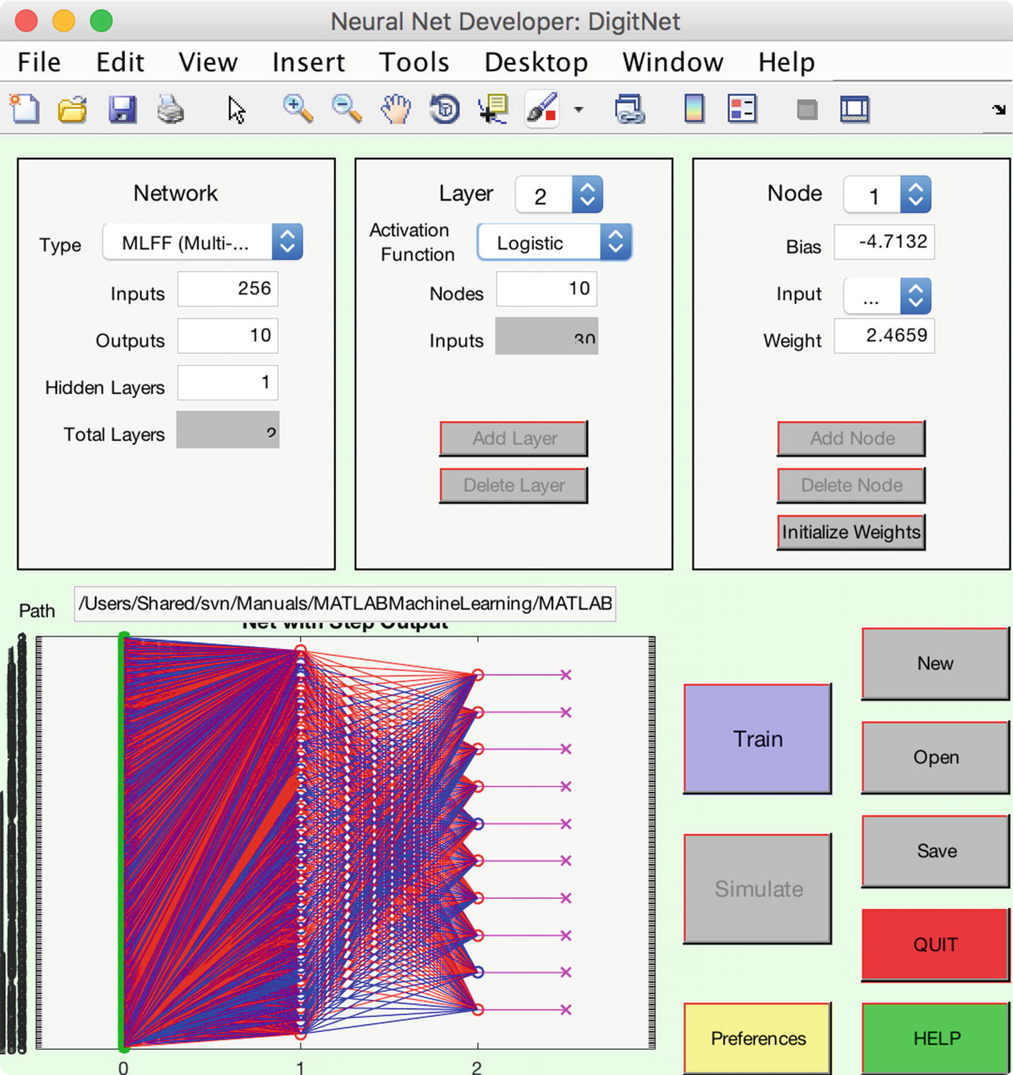
We can create this neural network with our GUI, shown in Figure 9.4. The network flows from left to right in the graphic. We can try training the net with the output node having different types, such as sign and logistic. In our case, we start with a sigmoid function for the hidden layer and a step function for the output node.
The box on the upper left of the GUI lets you set up the network with the number of inputs, in this case one per pixel, the number of outputs, one because we want to identify one digit, and the number of hidden layers. The box to the right lets us design each layer. All neurons in a layer are identical. The box on the far right lets us set the weight for each input to the node and the bias for the node. The path is the path to the training data. The display shows the resulting network. The graphic is useful, but the number of nodes in the hidden layer make it hard to read.
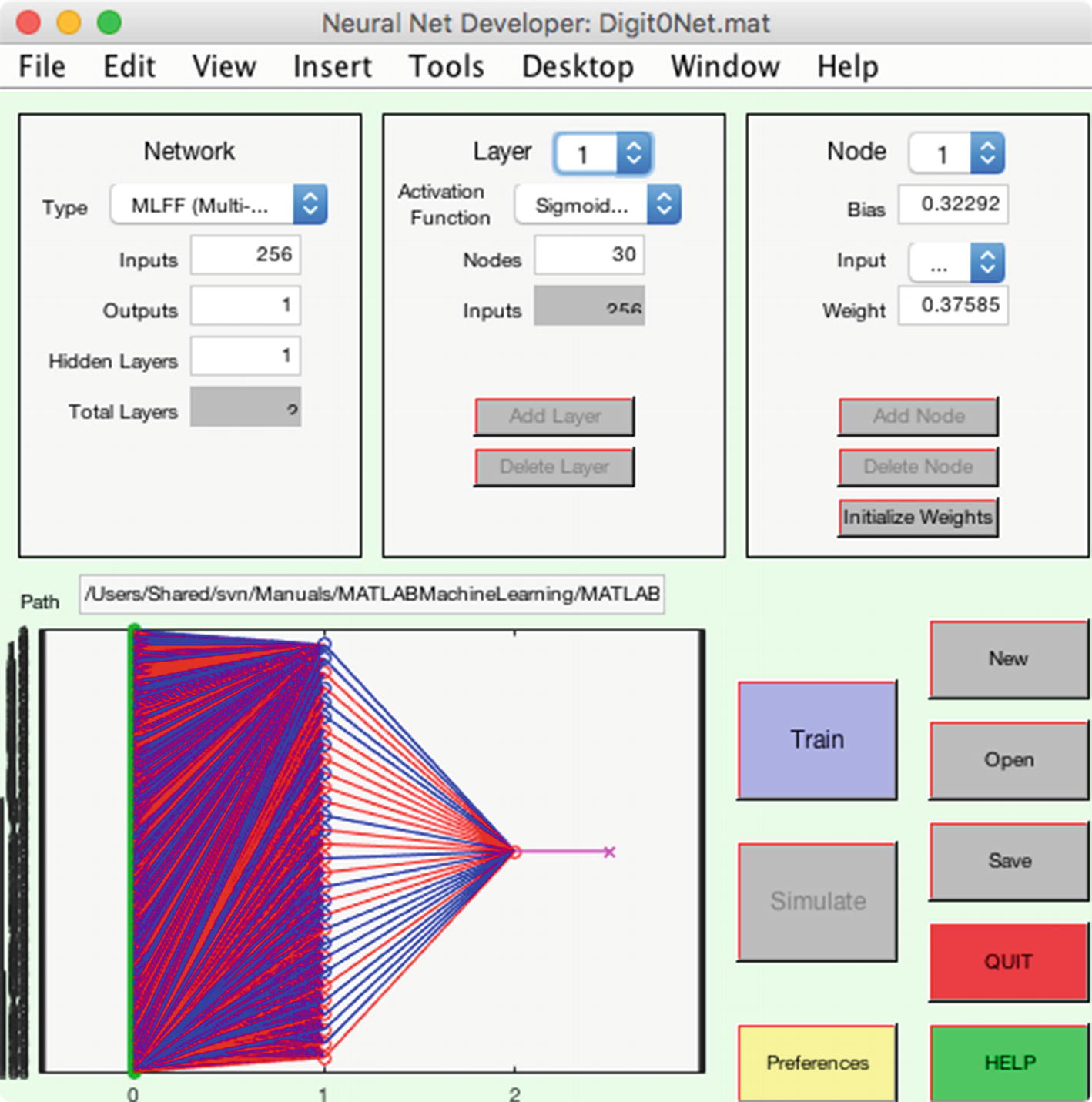
A neural net with 256 inputs, one per pixel, an intermediate layer with 30 nodes, and one output.
9.3.3 How It Works
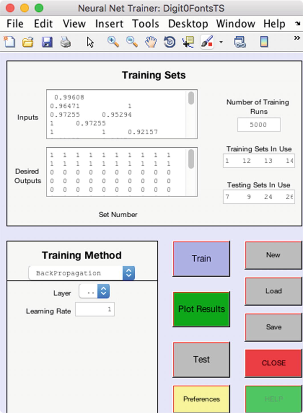
The neural net training GUI opens when the train button is clicked in the developer.
The training function also outputs the training error as the net evolves and the root mean square error (RMSE), which has dropped off to near 1e-2 by about run 1000.
Since we have a large number of input neurons, a line plot is not very useful for visualizing the evolution of the weights for the hidden layer. However, we can view the weights at any given iteration as an image. Figure 9.8 shows the weights for the network with 30 nodes after training visualized using imagesc. We may wonder if we really need all 30 nodes in the hidden layer, or if we could extract the necessary number of features identifying our chosen digit with fewer. In the image on the right, the weights are shown sorted along the dimension of the input pixels for each node; we can clearly see that only a few nodes seem to have much variation from the random values they are initialized with, especially nodes 14, 18, and 21. That is, many of our nodes seem to be having no impact.
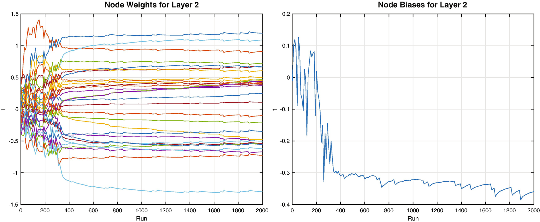
Layer 2 node weights and biases evolution during training.
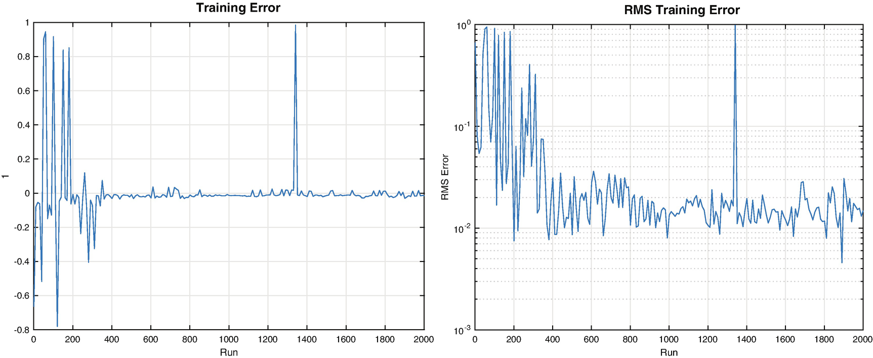
Single digit training error and RMSE
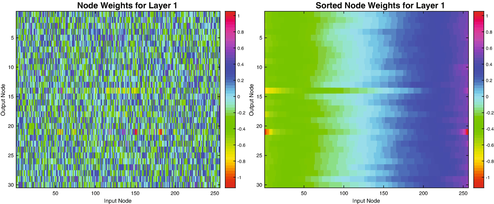
Single digit network, 30 node hidden layer weights. The plot on the left shows the weight value. The plot on the right shows the weights sorted by pixel for each node.
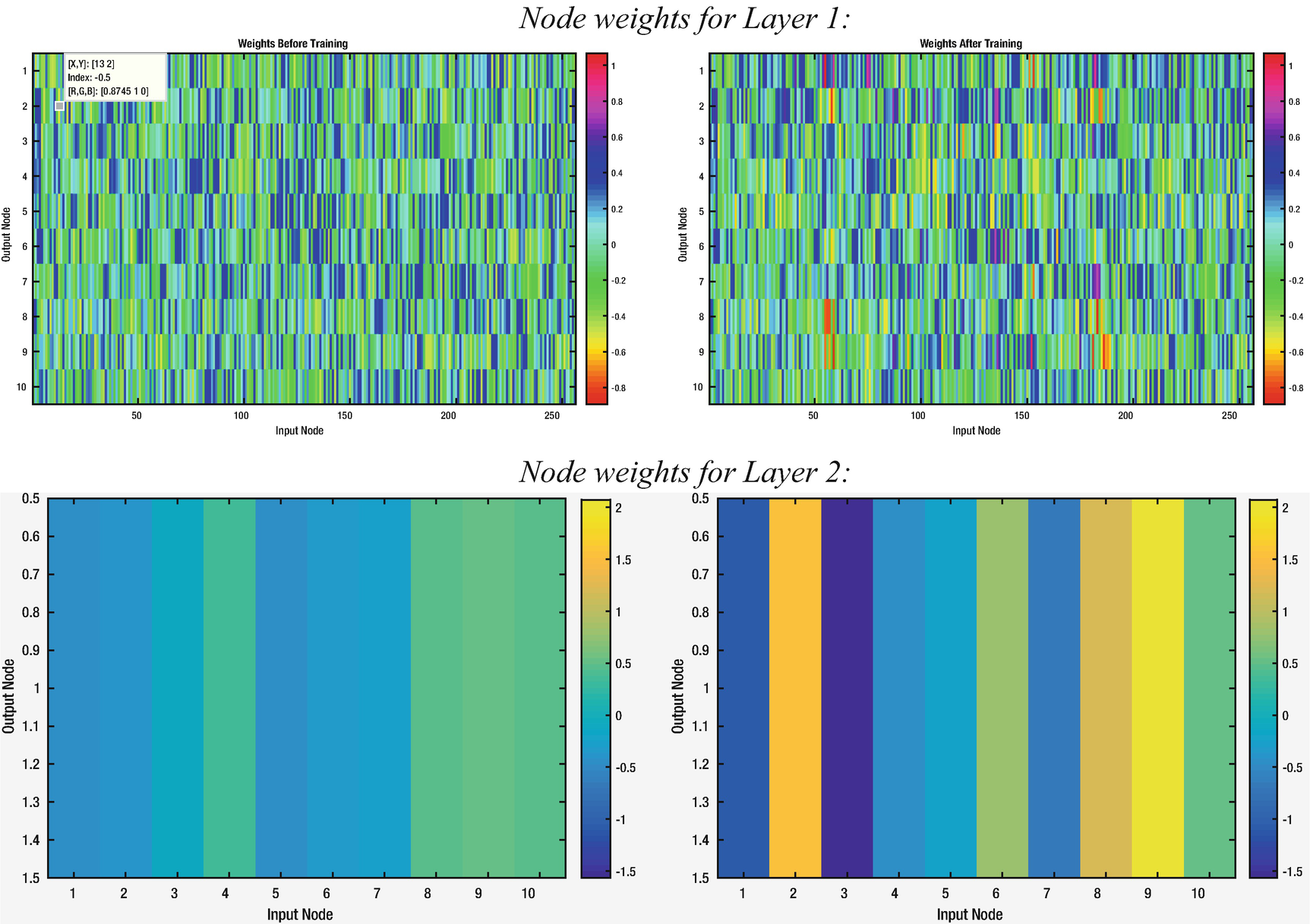
Single digit network, 10-node hidden layer weights before and after training. The first row shows the data for the first layer, and the second for the second layer, which has just one output.
Now we can see more patches of colors that have diverged from the initial random weights in the images for the 256 pixels weights, and we see clear variation in the weights for the second layer as well. The GUI allows you to save the trained net for future use.
9.4 Testing the Neural Network
9.4.1 Problem
We want to test the single-digit neural net that we trained in the previous recipe.
9.4.2 Solution
We can test the network with inputs that were not used in training. This is explicitly allowed in the GUI, as it has separate indices for the training data and testing data. We selected 75% of our sample images for training and saved the remaining images for testing in our DigitTrainingData script from Recipe 9.1.
9.4.3 How It Works
In the case of our GUI, simply click the test button to run the neural network with each of the cases selected for testing.
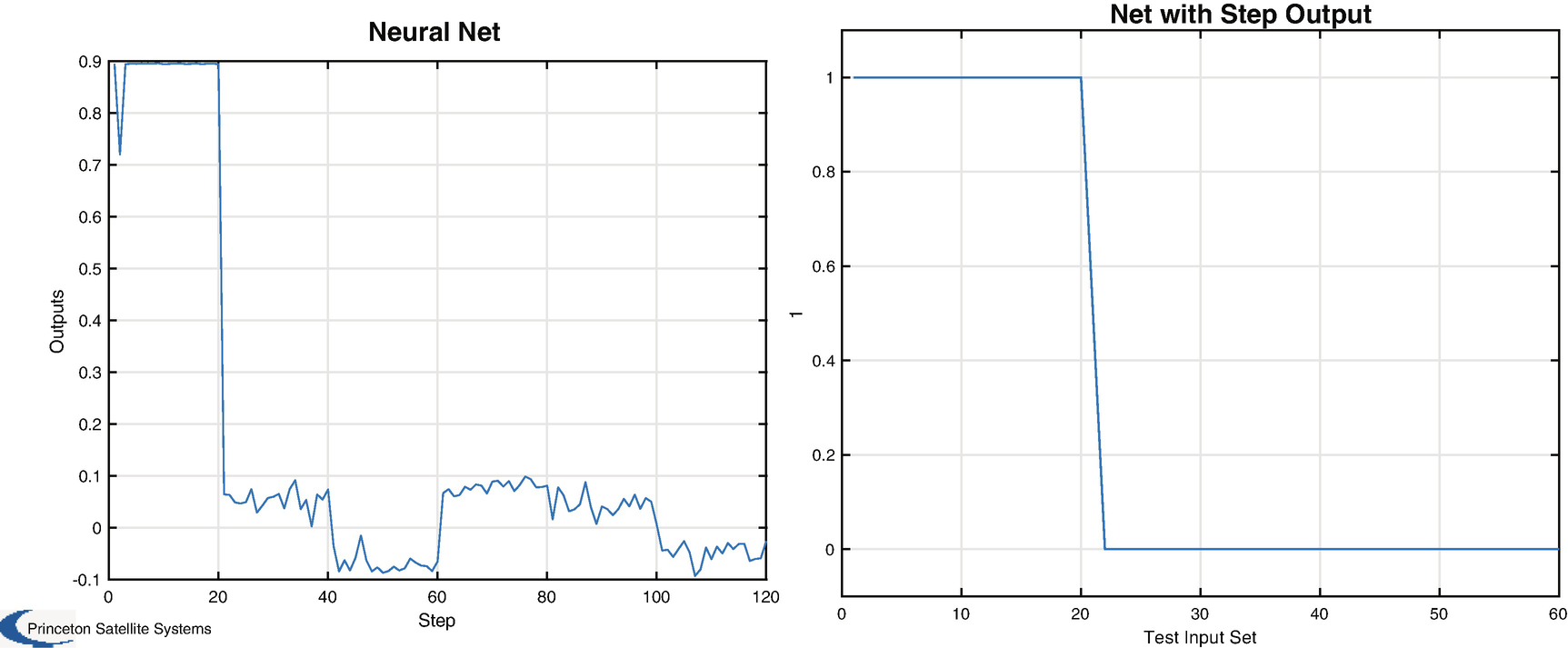
Neural net results with sigmoid (left) and step (right) activation functions.
9.5 Train a Network with Many Outputs
9.5.1 Problem
We want to build a neural net that can detect all ten digits separately.
9.5.2 Solution
Add nodes so that the output layer has ten nodes, each of which will be 0 or 1 when the representative digit (0–9) is input. Try the output nodes with different functions, such as logistic and step. Now that we have more digits, we will go back to having 30 nodes in the hidden layer.
9.5.3 How It Works
Our training data now consist of all 10 digits, with a binary output of zeros with a 1 in the correct slot. For example, the digit 1 will be represented as
[0 1 0 0 0 0 0 0 0]
The digit 3 would have a 1 in the fourth element. We follow the same procedure for training. We initialize the net, load the training set into the GUI, and specify the number of training runs for the back propagation.
Net with multiple outputs.
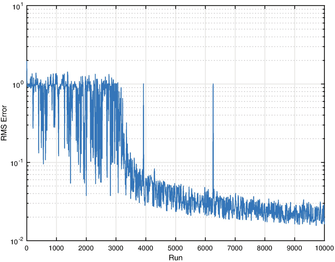
Training RMSE for a multiple-digit neural net.
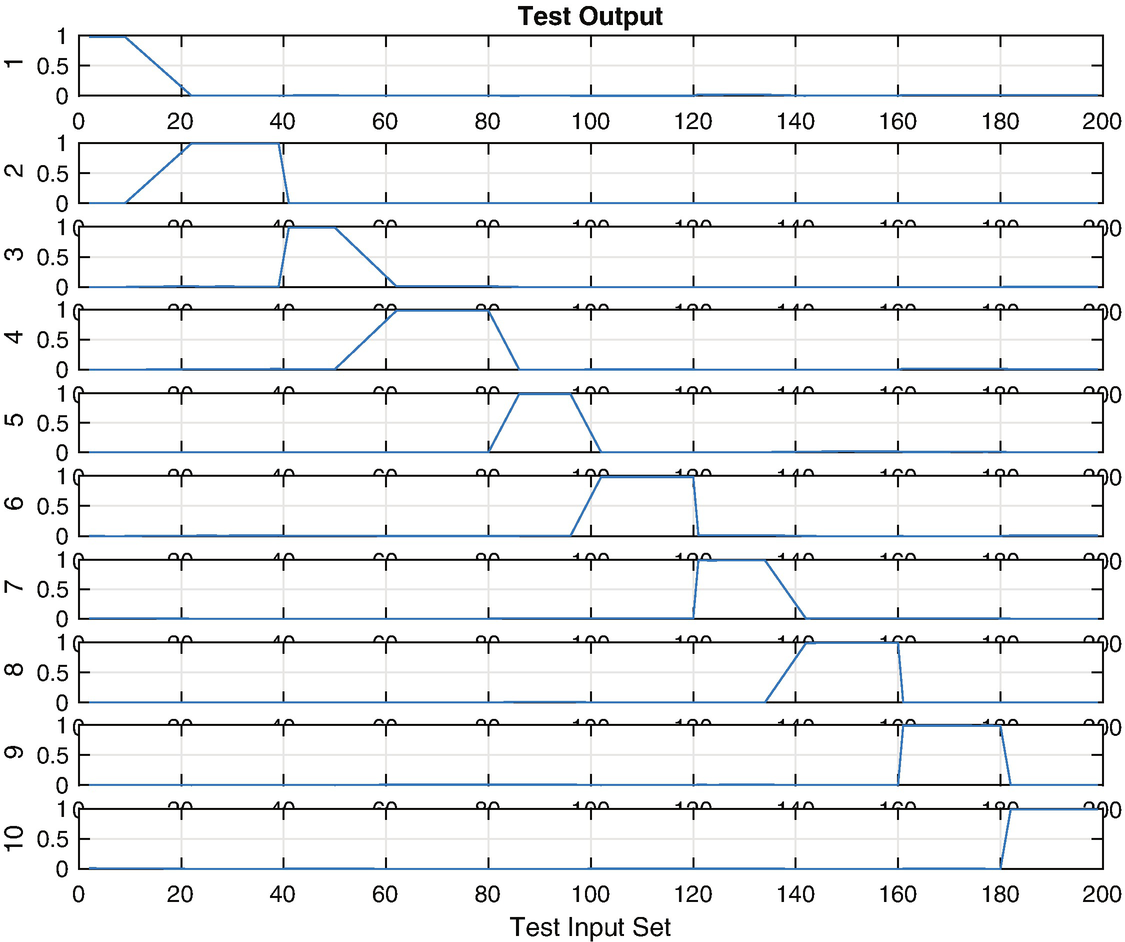
Test results for a multiple-digit neural net.
Once you have saved a net that is working well to a MAT-file, you can call it with new data using the function NeuralNetMLFF.
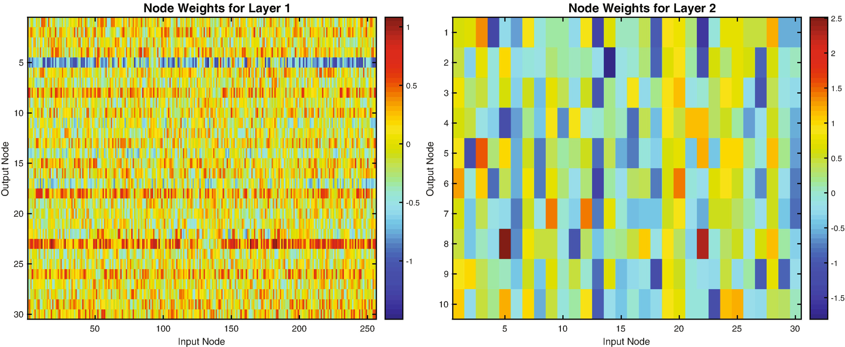
Multiple-digit neural net weights.
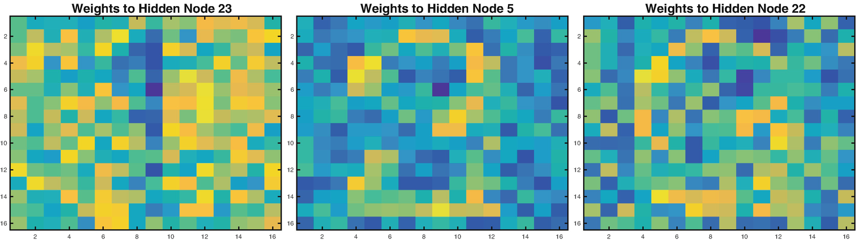
You can see parts of digits as mini-patterns in the individual node weights. Simply use imagesc with reshape like this:
Multiple-digit neural net weights.
9.6 Summary
Chapter Code Listing
File | Description |
|---|---|
DigitTrainingData | Create a training set of digit images. |
CreateDigitImage | Create a noisy image of a single digit. |
Neuron | Model an individual neuron with multiple activation functions. |
NeuralNetMLFF | Compute the output of a MLFF neural net. |
NeuralNetTraining | Training with back propagation. |
DrawNeuralNet | Display a neural net with multiple layers. |
SaveTS | Save a training set MAT-file with index data. |