© Michael Paluszek and Stephanie Thomas  2019
Michael Paluszek and Stephanie ThomasMATLAB Machine Learning Recipeshttps://doi.org/10.1007/978-1-4842-3916-2_4

4. Kalman Filters

Michael Paluszek1  and Stephanie Thomas1
(1)
Plainsboro, NJ, USA
 

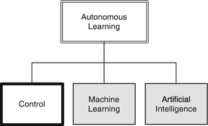
Understanding or controlling a physical system often requires a model of the system, that is, knowledge of the characteristics and structure of the system. A model can be a pre-defined structure or can be determined solely through data. In the case of Kalman Filtering, we create a model and use the model as a framework for learning about the system. This is part of the Control branch of our Autonomous Learning taxonomy from Chapter 1.

../images/420697_2_En_4_Chapter/420697_2_En_4_Figa_HTML.gif

What is important about Kalman Filters is that they rigorously account for uncertainty in a system that you want to know more about. There is uncertainty in the model of the system, if you have a model, and uncertainty (i.e., noise) in measurements of a system.

A system can be defined by its dynamical states and its parameters, which are nominally constant. For example, if you are studying an object sliding on a table, the states would be the position and velocity. The parameters would be the mass of the object and the friction coefficient. There may also be an external force on the object that we may want to estimate. The parameters and states comprise the model. You need to know both to properly understand the system. Sometimes it is hard to decide if something should be a state or a parameter. Mass is usually a parameter, but in a aircraft, car or rocket where the mass changes as fuel is consumed, it is often modeled as a state.

The Kalman Filters, invented by R. E. Kalman and others, are a mathematical framework for estimating or learning the states of a system. An estimator gives you statistically best estimates of the dynamical states of the system, such as the position and velocity of a moving point mass. Kalman Filters can also be written to identify the parameters of a system. Thus, the Kalman Filter provides a framework for both state and parameter identification.

Another application of Kalman Filters is system identification. System identification is the process of identifying the structure and parameters of any system. For example, with a simple mass on a spring it would be the identification or determination of the mass and spring constant values along with determining the differential equation for modeling the system. It is a form of machine learning that has its origins in control theory. There are many methods of system identification. In this chapter, we will only study the Kalman Filter. The term “learning” is not usually associated with estimation, but it is really the same thing.

An important aspect of the system identification problem is determining what parameters and states can actually be estimated given the measurements that are available. This applies to all learning systems. The question is, can we learn what we need to know about something through our observations? For this, we want to know if a parameter or state is observable and can be independently distinguished. For example, suppose we are using Newton’s law:
$$\displaystyle \begin{aligned} F = ma \end{aligned} $$
(4.1)
where F is force, m is mass, and a is acceleration as our model, and our measurement is acceleration. Can we estimate both force and mass? The answer is no, because we are measuring the ratio of force to mass
$$\displaystyle \begin{aligned} a = \frac{F}{m} \end{aligned} $$
(4.2)
We can’t separate the two. If we had a force sensor or a mass sensor we could determine each separately. You need to be aware of this issue in all learning systems, including Kalman Filters.

4.1 A State Estimator Using a Linear Kalman Filter

4.1.1 Problem

You want to estimate the velocity and position of a mass attached through a spring and damper to a structure. The system is shown in Figure 4.1. m is the mass, k is the spring constant, c is the damping constant, and f is an external force. x is the position. The mass moves in only one direction.

Suppose we had a camera that was located near the mass. The camera would be pointed at the mass during its ascent. This would result in a measurement of the angle between the ground and the boresight of the camera. The angle measurement geometry is shown in Figure 4.2. The angle is measured from an offset baseline.

We want to use a conventional linear Kalman Filter to estimate the state of the system. This is suitable for a simple system that can be modeled with linear equations.
../images/420697_2_En_4_Chapter/420697_2_En_4_Fig1_HTML.png
Figure 4.1

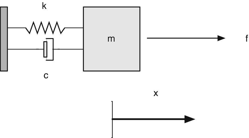
Spring-mass-damper system. The mass is on the right. The spring is on the top to the left of the mass. The damper is below.

../images/420697_2_En_4_Chapter/420697_2_En_4_Fig2_HTML.png
Figure 4.2

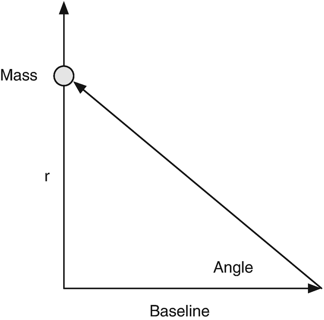
The angle measurement geometry.

4.1.2 Solution

First, we will need to define a mathematical model for the mass system and code it up. Then we will derive the Kalman Filter from first principles, using Bayes theorem. Finally, we present code implementing the Kalman Filter estimator for the spring-mass problem.

4.1.3 How It Works

Spring-Mass System Model

The continuous time differential equations modeling the system are
$$\displaystyle \begin{aligned} \begin{array}{rcl} \frac{dr}{dt} &\displaystyle =&\displaystyle v \end{array} \end{aligned} $$
(4.3)
$$\displaystyle \begin{aligned} \begin{array}{rcl} m\frac{dv}{dt}&\displaystyle =&\displaystyle f - cv - kx \end{array} \end{aligned} $$
(4.4)
This says the change in position r with respect to time t is the velocity v. The change in velocity with respect to time (times mass) is an external force, minus the damping constant times velocity, minus the spring constant times the position. The second equation is just Newton’s law where the total force is F and the total acceleration, aT, is the total force divided by the mass, $$\frac {F}{m}$$
$$\displaystyle \begin{aligned} \begin{array}{rcl} F &\displaystyle =&\displaystyle f - cv - kx \end{array} \end{aligned} $$
(4.5)
$$\displaystyle \begin{aligned} \begin{array}{rcl} \frac{dv}{dt}&\displaystyle =&\displaystyle a_T \end{array} \end{aligned} $$
(4.6)
To simplify the problem we divide both sides of the second equation by mass and get:
$$\displaystyle \begin{aligned} \begin{array}{rcl} \frac{dr}{dt} &\displaystyle =&\displaystyle v \end{array} \end{aligned} $$
(4.7)
$$\displaystyle \begin{aligned} \begin{array}{rcl} \frac{dv}{dt}&\displaystyle =&\displaystyle a - 2\zeta\omega v - \omega^2x \end{array} \end{aligned} $$
(4.8)
where
$$\displaystyle \begin{aligned} \begin{array}{rcl} \frac{c}{m} &\displaystyle =&\displaystyle 2\zeta\omega \end{array} \end{aligned} $$
(4.9)
$$\displaystyle \begin{aligned} \begin{array}{rcl} \frac{k}{m} &\displaystyle =&\displaystyle \omega^2 \end{array} \end{aligned} $$
(4.10)
a is the acceleration due to external forces $$\frac {f}{m}$$, ζ is the damping ratio, and ω is the undamped natural frequency. The undamped natural frequency is the frequency at which the mass would oscillate if there were no damping. The damping ratio indicates how fast the system damps and what level of oscillations we observe. With a damping ratio of zero, the system never damps and the mass oscillates forever. With a damping ratio of one you don’t see any oscillation. This form makes it easier to understand what damping and oscillation to expect. You immediately know the frequency and the rate at which the oscillation should subside. m, c, and k, although they embody the same information, don’t make this as obvious.

The following shows a simulation of the oscillator with damping (OscillatorDamping RatioSim). It shows different damping ratios. The loop that runs the simulation with different damping ratios is shown.

for j = 1:length(zeta)
    % Initial state [position;velocity]
   x = [0;1];
    % Select damping ratio from array
   d.zeta= zeta(j);
    % Print a string for the legend
   s{j} =  sprintf ( ’zeta␣=␣%6.4f’,zeta(j));
    for k = 1:nSim
      % Plot storage
     xPlot(j,k)  = x(1);
      % Propagate (numerically integrate) the state equations
     x  = RungeKutta( @RHSOscillator, 0, x, dT, d );
    end
end
The results of the damping ratio demo are shown in Figure 4.3. The initial conditions are zero position and a velocity of one. The responses to different levels of damping ratios are seen. When zeta is zero it is undamped and oscillates forever. Critical damping, which is desirable from minimizing actuator effort, is 0.7071. A damping ratio of 1 results in no overshoot to a step disturbance. In this case, we have “overshoot,” since we are not at a rest initial condition.
../images/420697_2_En_4_Chapter/420697_2_En_4_Fig3_HTML.png
Figure 4.3

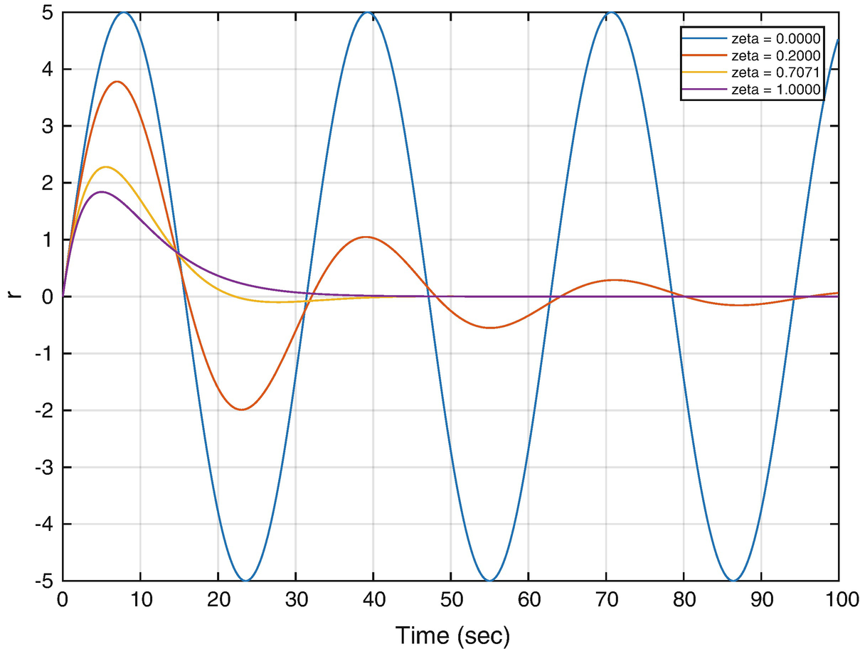
Spring-mass-damper system simulation with different damping ratios zeta.

The dynamical equations are in what is called state-space form because the derivative of the state vector:
$$\displaystyle \begin{aligned} x = \left[ \begin{array}{r} r\\ v \end{array} \right] \end{aligned} $$
(4.11)
has nothing multiplying it and there are only first derivatives on the left-hand side. Sometimes you see equations like:
$$\displaystyle \begin{aligned} Q\dot{x} = Ax + Bu \end{aligned} $$
(4.12)
If Q is not invertible then you can’t do:
$$\displaystyle \begin{aligned} \dot{x} = Q^{-1}Ax + Q^{-1}Bu \end{aligned} $$
(4.13)
to make state space equations. Conceptually, if Q is not invertible, that is the same thing as having fewer than N unique equations (where N is the length of x, the number of states).

All of our filter derivations work with dynamical equations in state space form. Also, most numerical integration schemes are designed for sets of first-order differential equations.

The right-hand side for the state equations (first-order differential equations), RHSOscillator, is shown in the following listing. Notice that if no inputs are requested, it returns the default data structure. The code, if ( nargin <1), tells the function to return the data structure if no inputs are given. This is a convenient way of making your functions self-documenting and keeping your data structures consistent. The actual working code is just one line.

 xDot = [x(2);d.a-2*d.zeta*d.omega*x(2)-d.omega^2*x(1)];  

The following listing gives the simulation script OscillatorSim. It causes the right-hand side, RHSOscillator, to be numerically integrated using the RungeKutta function. We start by getting the default data structure from the right-hand side. We fill it in with our desired parameters. Measurements y are created for each step, including random noise. There are two measurements: position and angle.

The following code shows just the simulation loop of OscillatorSim. The angle measurement is just trigonometry. The first measurement line computes the angle, which is a nonlinear measurement. The second measures the vertical distance, which is linear.

for k = 1:nSim
    % Measurements
   yTheta =  atan (x(1)/baseline) + yTheta1Sigma* randn (1,1);
   yR     = x(1) + yR1Sigma* randn (1,1);
    % Plot storage
   xPlot(:,k) = [x;yTheta;yR];
    % Propagate (numerically integrate) the state equations
   x = RungeKutta( @RHSOscillator, 0, x, dT, dRHS );
end
The results of the simulation are shown in Figure 4.4. The input is a disturbance acceleration that goes from zero to its value at time t = 0. It is constant for the duration of the simulation. This is known as a step disturbance. This causes the system to oscillate. The magnitude of the oscillation slowly goes to zero because of the damping. If the damping ratio were 1, we would not see any oscillation, as seen in Figure 4.3.
../images/420697_2_En_4_Chapter/420697_2_En_4_Fig4_HTML.png
Figure 4.4

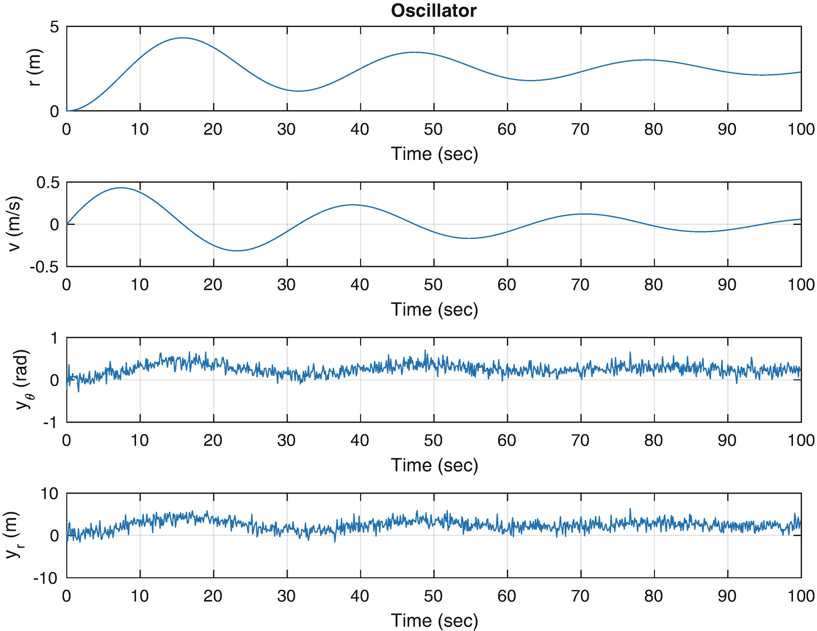
Spring-mass-damper system simulation. The input is a step acceleration. The oscillation slowly damps out, that is, it goes to zero over time. The position r develops an offset due to the constant acceleration.

The offset seen in the plot of r can be found analytically by setting v = 0. Essentially, the spring force is balancing the external force.
$$\displaystyle \begin{aligned} \begin{array}{rcl} 0 =\frac{dv}{dt}= a - \omega^2x \end{array} \end{aligned} $$
(4.14)
$$\displaystyle \begin{aligned} \begin{array}{rcl} x = \frac{a}{\omega^2} \end{array} \end{aligned} $$
(4.15)
We have now completed the derivation of our model and can move on to building the Kalman Filters.

Kalman Filter Derivation

Kalman filters can be derived from Bayes’ Theorem. What is Bayes’ Theorem? Bayes’ Theorem is:
$$\displaystyle \begin{aligned} \begin{array}{rcl} P(A_i|B) = \frac{P(B|A_i)P(A_i)}{\sum P(B|A_i)} \end{array} \end{aligned} $$
(4.16)
$$\displaystyle \begin{aligned} \begin{array}{rcl} P(A_i|B)= \frac{P(B|A_i)P(A_i)}{P(B)} \end{array} \end{aligned} $$
(4.17)
which is just the probability of Ai given B. P means “probability.” The vertical bar | means “given.” This assumes that the probability of B is not zero, that is, P(B)≠0. In the Bayesian interpretation, the theorem introduces the effect of evidence on belief. This provides a rigorous framework for incorporating any data for which there is a degree of uncertainty. Put simply, given all evidence (or data) to date, Bayes’ Theorem allows you to determine how new evidence affects the belief. In the case of state estimation this is the belief in the accuracy of the state estimate.

Figure 4.5 shows the Kalman Filter family and how it relates to the Bayesian Filter. In this book we are covering only the ones in the colored boxes. The complete derivation of the Kalman Filter is given below; this provides a coherent framework for all Kalman filtering implementations. The different filters fall out of the Bayesian models based on assumptions about the model and sensor noise and the linearity or nonlinearity of the measurement and dynamics models. Let’s look at the branch that is colored blue. Additive Gaussian noise filters can be linear or nonlinear depending on the type of dynamical and measurement models. In many cases you can take a nonlinear system and linearize it about the normal operating conditions. You can then use a linear Kalman Filter. For example, a spacecraft dynamical model is nonlinear and an Earth sensor that measures the Earth’s chord width for roll and pitch information is nonlinear. However, if we are only concerned with Earth pointing, and small deviations from nominal pointing, we can linearize both the dynamical equations and the measurement equations and use a linear Kalman Filter.

If nonlinearities are important, we have to use a nonlinear filter. The Extended Kalman Filter (EKF) uses partial derivatives of the measurement and dynamical equations. These are computed each time step or with each measurement input. In effect, we are linearizing the system each step and using the linear equations. We don’t have to do a linear state propagation, that is, propagating the dynamical equations, and could propagate them using numerical integration. If we can get analytical derivatives of the measurement and dynamical equations, this is a reasonable approach. If there are singularities in any of the equations, this may not work.

The Unscented Kalman Filter (UKF) uses the nonlinear equations directly. There are two forms, augmented and non-augmented. In the former, we created an augmented state vector that includes both the states and the state and measurement noise variables. This may result in better results at the expense of more computation.

All of the filters in this chapter are Markov, that is, the current dynamical state is entirely determined from the previous state. Particle filters are not addressed in this book. They are a class of Monte Carlo methods. Monte Carlo (named after the famous casino) methods are computational algorithms that rely on random sampling to obtain results. For example, a Monte Carlo approach to our oscillator simulation would be to use the MATLAB function nrandn to generate the accelerations. We’d run many tests to verify that our mass moves as expected.
../images/420697_2_En_4_Chapter/420697_2_En_4_Fig5_HTML.png
Figure 4.5

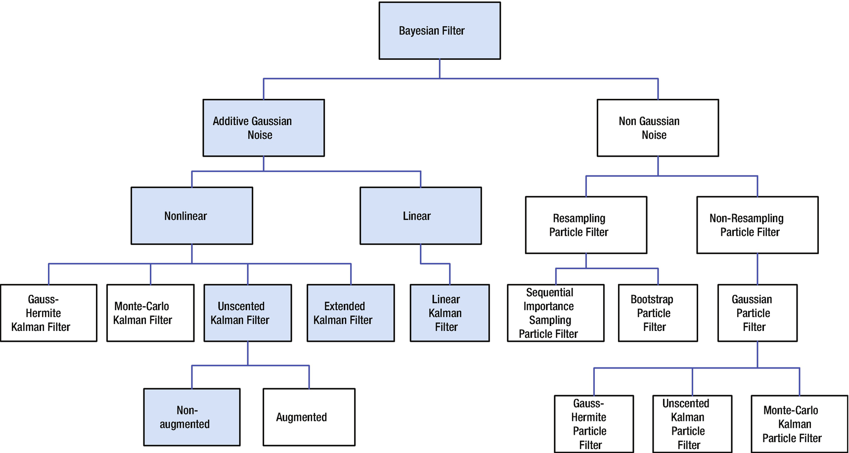
The Kalman Filter family tree. All are derived from a Bayesian filter. This chapter covers those in colored boxes.

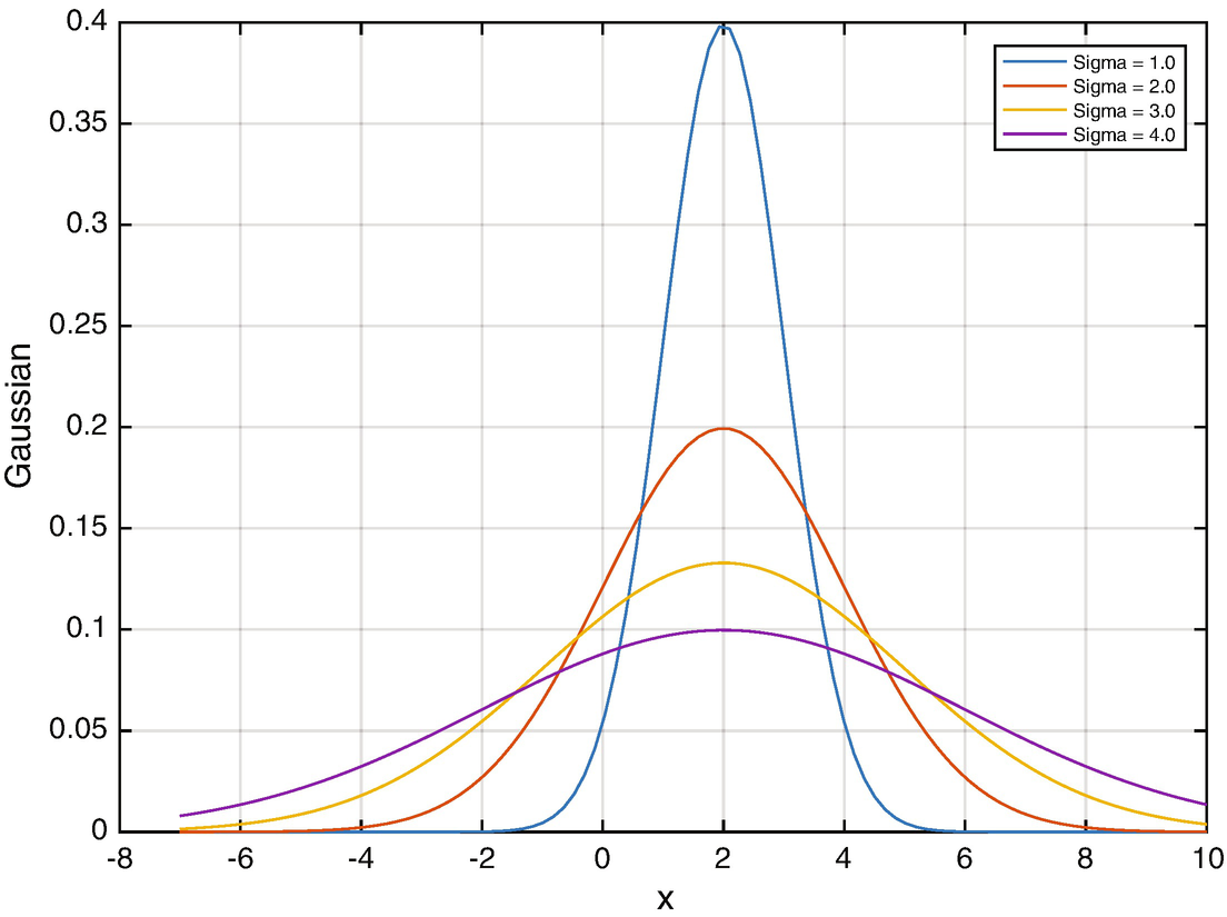
Our derivation will use the notation N(μ, σ 2) to represent a normal variable. A normal variable is another word for a Gaussian variable. Gaussian means it is distributed as the normal distribution with mean μ (average) and variance σ 2. The following code from Gaussian computes a Gaussian or Normal distribution around a mean of 2 for a range of standard deviations. Figure 4.6 shows a plot. The height of the plot indicates how likely a given measurement of the variable is to have that value.

  %% Initialize
 mu            = 2;            % Mean
 sigma         = [1 2 3 4];  % Standard deviation
 n             =  length (sigma);
 x             =  linspace (-7,10);
  %% Simulation
 xPlot =  zeros (n, length (x));
 s     =  cell (1,n);
for k = 1:length(sigma)
   s{k}       =  sprintf ( ’Sigma␣=␣%3.1f’,sigma(k));
   f          = -(x-mu).^2/(2*sigma(k)^2);
   xPlot(k,:) =  exp (f)/ sqrt (2* pi *sigma(k)^2);
end
../images/420697_2_En_4_Chapter/420697_2_En_4_Fig6_HTML.png
Figure 4.6

Normal or Gaussian random variable about a mean of 2.

Given the probabilistic state space model in discrete time [23]
$$\displaystyle \begin{aligned} x_k = f_k(x_{k-1},w_{k-1}) \end{aligned} $$
(4.18)
where x is the state vector and w is the noise vector, the measurement equation is:
$$\displaystyle \begin{aligned} y_k = h_k(x_k,v_n) \end{aligned} $$
(4.19)
where vn is the measurement noise. This has the form of a hidden Markov model (HMM) because the state is hidden.
If the process is Markovian, then the future state xk is dependent only on the current state xk−1 and is not dependent on the past states. This can be expressed in the equation:
$$\displaystyle \begin{aligned} p(x_k|x_{1:k-1},y_{1:k-1}) = p(x_k|x_{k-1}) \end{aligned} $$
(4.20)
The | means given. In this case, the first term is read as “the probability of xk given x 1:k−1 and y 1:k−1.” This is the probability of the current state given all past states and all measurements up to the k − 1 measurement. The past, xk−1, is independent of the future given the present.
$$\displaystyle \begin{aligned} p(x_{k-1}|x_{k:T},y_{k:T}) = p(x_{k-1}|x_k) \end{aligned} $$
(4.21)
where T is the last sample and the measurements yk are conditionally independent given xk; that is, they can be determined using only xk and are not dependent on x 1:k or y 1:k−1. This can be expressed as:
$$\displaystyle \begin{aligned} p(y_k|x_{1:k},y_{1:k-1}) = p(y_k|x_k) \end{aligned} $$
(4.22)
We can define the recursive Bayesian optimal filter that computes the distribution:
$$\displaystyle \begin{aligned} p(x_k|y_{1:k}) \end{aligned} $$
(4.23)
given:
  • The prior distribution p(x 0), where x 0 is the state prior to the first measurement,

  • The state space model
    $$\displaystyle \begin{aligned} \begin{array}{rcl} x_k &amp;\displaystyle \sim&amp;\displaystyle p(x_k|x_{k-1}) \end{array} \end{aligned} $$
    (4.24)
    $$\displaystyle \begin{aligned} \begin{array}{rcl} y_k &amp;\displaystyle \sim&amp;\displaystyle p(y_k|x_k) \end{array} \end{aligned} $$
    (4.25)
  • The measurement sequence y 1:k = y 1, …, yk.

Computation is based on the recursion rule
$$\displaystyle \begin{aligned} p(x_{k-1}|y_{1:k-1}) \rightarrow p(x_k|y_{1:k}) \end{aligned} $$
(4.26)
This means that we get the current state xk from the prior state xk−1 and all the past measurements y 1:k−1. Assume that we know the posterior distribution of the previous time step:
$$\displaystyle \begin{aligned} p(x_{k-1}|y_{1:k-1}) \end{aligned} $$
(4.27)
The joint distribution of xk, xk−1 given y 1:k−1 can be computed as:
$$\displaystyle \begin{aligned} \begin{array}{rcl} p(x_k,x_{k-1}|y_{1:k-1}) &amp;\displaystyle =&amp;\displaystyle p(x_k|x_{k-1},y_{1:k-1})p(x_{k-1}|y_{1:k-1}) \end{array} \end{aligned} $$
(4.28)
$$\displaystyle \begin{aligned} \begin{array}{rcl} &amp;\displaystyle =&amp;\displaystyle p(x_k|x_{k-1})p(x_{k-1}|y_{1:k-1}) \end{array} \end{aligned} $$
(4.29)
because this is a Markov process. Integrating over xk−1 gives the prediction step of the optimal filter, which is the Chapman–Kolmogorov equation
$$\displaystyle \begin{aligned} p(x_k|y_{1:k-1}) = \int p(x_k|x_{k-1},y_{1:k-1})p(x_{k-1}|y_{1:k-1})dx_{k-1} \end{aligned} $$
(4.30)
The Chapman–Kolmogorov equation is an identity relating the joint probability distributions of different sets of coordinates on a stochastic process. The measurement update state is found from Bayes’ Rule:
$$\displaystyle \begin{aligned} \begin{array}{rcl} P(x_k|y_{1:k}) = \frac{1}{C_k} p(y_k|x_k)p(x_k|y_{k-1})&amp;\displaystyle &amp;\displaystyle \end{array} \end{aligned} $$
(4.31)
$$\displaystyle \begin{aligned} \begin{array}{rcl} C_k = p(y_k|y_{1:k-1}) = \int p(y_k|x_k)p(x_k|y_{1:k-1})dx_k&amp;\displaystyle &amp;\displaystyle \end{array} \end{aligned} $$
(4.32)
Ck is the probability of the current measurement, given all past measurements.
If the noise is additive and Gaussian with the state covariance Qn and the measurement covariance Rn, the model and measurement noise have zero mean, and we can write the state equation as:
$$\displaystyle \begin{aligned} x_k = f_k(x_{k-1}) +w_{k-1} \end{aligned} $$
(4.33)
where x is the state vector and w is the noise vector. The measurement equation becomes:
$$\displaystyle \begin{aligned} y_k = h_k(x_k) + v_n \end{aligned} $$
(4.34)
Given that Q is not time-dependent we can write:
$$\displaystyle \begin{aligned} p (x_k|x_{k-1}, y_{1:k-1}) = {N} (x_k; f (x_{k-1}) , Q) \end{aligned} $$
(4.35)
where recall that N is a normal variable, in this case, with mean xk;f(xk−1), which means (xk given f(xk−1) and variance Q. We can now write the prediction step Equation 4.30 as:
$$\displaystyle \begin{aligned} p(x_k|y_{1:k-1}) = \int {N} (x_k; f (x_{k-1}) , Q) p(x_{k-1}|y_{1:k-1})dx_{k-1} \end{aligned} $$
(4.36)
We need to find the first two moments of xk. A moment is the expected value (or mean) of the variable. The first moment is of the variable, the second is of the variable squared and so forth. They are:
$$\displaystyle \begin{aligned} \begin{array}{rcl} E[x_k] = \int x_k p(x_k|y_{1:k-1}) dx_k &amp;\displaystyle &amp;\displaystyle \end{array} \end{aligned} $$
(4.37)
$$\displaystyle \begin{aligned} \begin{array}{rcl} E[x_kx_k^T] = \int x_kx_k^T p(x_k|y_{1:k-1}) dx_k&amp;\displaystyle &amp;\displaystyle \end{array} \end{aligned} $$
(4.38)
E means expected value. E[xk] is the mean and $$E[x_kx_k^T] $$ is the covariance. Expanding the first moment and using the identity $$E[x] = \int x {N}(x;f(s),\varSigma )dx = f(s)$$ where s is any argument.
$$\displaystyle \begin{aligned} \begin{array}{rcl} E[x_k] &amp;\displaystyle =&amp;\displaystyle \int x_k\left[ \int \mathrm{d} (x_k; f (x_{k-1}) , Q) p(x_{k-1}|y_{1:k-1})dx_{k-1} \right]dx_k \end{array} \end{aligned} $$
(4.39)
$$\displaystyle \begin{aligned} \begin{array}{rcl} &amp;\displaystyle =&amp;\displaystyle \int x_k\left[ \int {N}(x_k; f (x_{k-1}) , Q) dx_k\right]p(x_{k-1}|y_{1:k-1})dx_{k-1} \end{array} \end{aligned} $$
(4.40)
$$\displaystyle \begin{aligned} \begin{array}{rcl} &amp;\displaystyle =&amp;\displaystyle \int f (x_{k-1}) p(x_{k-1}|y_{1:k-1})dx_{k-1} \end{array} \end{aligned} $$
(4.41)
Assuming that $$ p(x_{k-1}|y_{1:k-1}) = {N}(x_{k-1};\hat {x}_{k-1|k-1},P^{xx}_{k-1|k-1})$$ where Pxx is the covariance of x and noting that xk = fk(xk−1) + wk−1 we get:
$$\displaystyle \begin{aligned} \hat{x}_{k|k-1}= \int f(x_{k-1}) {N}(x_{k-1};\hat{x}_{k-1|k-1},P^{xx}_{k-1|k-1})dx_{k-1} \end{aligned} $$
(4.42)
For the second moment:
$$\displaystyle \begin{aligned} \begin{array}{rcl} E[x_kx_k^T] &amp;\displaystyle =&amp;\displaystyle \int x_kx_k^T p(x_k|y_{1:k-1}) dx_k \end{array} \end{aligned} $$
(4.43)
$$\displaystyle \begin{aligned} \begin{array}{rcl} &amp;\displaystyle =&amp;\displaystyle \int \left[ \int {N}(x_k; f (x_{k-1}) , Q) x_kx_k^Tdx_k\right]p(x_{k-1}|y_{1:k-1})dx_{k-1} \end{array} \end{aligned} $$
(4.44)
which results in:
$$\displaystyle \begin{aligned} P^{xx}_{k|k-1} = Q + \int f(x_{k-1}) f^T(x_{k-1}) {N}(x_{k-1};\hat{x}_{k-1|k-1},P^{xx}_{k-1|k-1})dx_{k-1} - \hat{x}^T_{k|k-1} \hat{x}_{k|k-1} \end{aligned} $$
(4.45)
The covariance for the initial state is Gaussian and is $$P^{xx}_0$$. The Kalman Filter can be written without further approximations as
$$\displaystyle \begin{aligned} \begin{array}{rcl} \hat{x}_{k|k} &amp;\displaystyle =&amp;\displaystyle \hat{x}_{k|k-1} + K_n\left[y_k - \hat{y}_{k|k-1}\right] \end{array} \end{aligned} $$
(4.46)
$$\displaystyle \begin{aligned} \begin{array}{rcl} P^{xx}_{k|k} &amp;\displaystyle =&amp;\displaystyle P^{xx}_{k|k-1} - K_nP^{yy}_{k|k-1}K^T_n \end{array} \end{aligned} $$
(4.47)
$$\displaystyle \begin{aligned} \begin{array}{rcl} K_n &amp;\displaystyle =&amp;\displaystyle P^{xy}_{k|k-1}\left[ P^{yy}_{k|k-1}\right]^{-1} \end{array} \end{aligned} $$
(4.48)
where Kn is the Kalman gain and Pyy is the measurement covariance. The solution of these equations requires the solution of five integrals of the form:
$$\displaystyle \begin{aligned} I = \int g(x) {N}(x;\hat{x},P^{xx})dx \end{aligned} $$
(4.49)
The three integrals needed by the filter are:
$$\displaystyle \begin{aligned} \begin{array}{rcl} P^{yy}_{k|k-1} &amp;\displaystyle =&amp;\displaystyle R + \int h(x_{n}) h^T(x_{n}) {N}(x_{n};\hat{x}_{k|k-1},P^{xx}_{k|k-1})dx_k - \hat{x}^T_{k|k-1} \hat{y}_{k|k-1} \end{array} \end{aligned} $$
(4.50)
$$\displaystyle \begin{aligned} \begin{array}{rcl} P^{xy}_{k|k-1} &amp;\displaystyle =&amp;\displaystyle \int x_{n}h^T(x_{n}){N}(x_{n};\hat{x}_{k|k-1},P^{xx}_{k|k-1})dx \end{array} \end{aligned} $$
(4.51)
$$\displaystyle \begin{aligned} \begin{array}{rcl} \hat{y}_{k|k-1} &amp;\displaystyle =&amp;\displaystyle \int h(x_k) {N}(x_k;\hat{x}_{k|k-1},P^{xx}_{k|k-1})dx_k \end{array} \end{aligned} $$
(4.52)
Assume that we have a model of the form:
$$\displaystyle \begin{aligned} \begin{array}{rcl} x_k &amp;\displaystyle =&amp;\displaystyle A_{k-1}x_{k-1} + B_{k-1}u_{k-1} + q_{k-1} \end{array} \end{aligned} $$
(4.53)
$$\displaystyle \begin{aligned} \begin{array}{rcl} y_k &amp;\displaystyle =&amp;\displaystyle H_kx_k + r_{k} \end{array} \end{aligned} $$
(4.54)
where
  • $$x_k \in \Re ^n$$ is the state of system at time k

  • mk is the mean state at time k

  • Ak−1 is the state transition matrix at time k − 1

  • Bk − 1 is the input matrix at time k − 1

  • uk − 1 is the input at time k − 1

  • qk−1, N(0, Qk), is the Gaussian process noise at time k − 1

  • $$y_k \in \Re ^m$$ is the measurement at time k

  • Hk is the measurement matrix at time k. This is found from the Jacobian (derivatives) of h(x).

  • rk = N(0, Rk), is the Gaussian measurement noise at time k

  • The prior distribution of the state is x 0 = N(m 0, P 0) where parameters m 0 and P 0 contain all prior knowledge about the system. m 0 is the mean at time zero and P 0 is the covariance. Since our state is Gaussian, this completely describes the state.

  • $$\hat {x}_{k|k-1}$$ is the mean of x at k given $$\hat {x}$$ at k − 1

  • $$\hat {y}_{k|k-1}$$ is the mean of y at k given $$\hat {x}$$ at k − 1

$$\Re ^n$$ means real numbers in a vector of order n, that is, the state has n quantities. In probabilistic terms the model is:
$$\displaystyle \begin{aligned} \begin{array}{rcl} p(x_k|x_{k-1}) &amp;\displaystyle =&amp;\displaystyle {N}(x_k;A_{k-1}x_{k-1},Q_k) \end{array} \end{aligned} $$
(4.55)
$$\displaystyle \begin{aligned} \begin{array}{rcl} p(y_k|x_k) &amp;\displaystyle =&amp;\displaystyle {N}(y_k;H_kx_k,R_k) \end{array} \end{aligned} $$
(4.56)
The integrals become simple matrix equations. In the following equations, $$P_k^- $$ means the covariance prior to the measurement update.
$$\displaystyle \begin{aligned} \begin{array}{rcl} P^{yy}_{k|k-1} &amp;\displaystyle =&amp;\displaystyle H_kP_k^- H_k^T+R_{k} \end{array} \end{aligned} $$
(4.57)
$$\displaystyle \begin{aligned} \begin{array}{rcl} P^{xy}_{k|k-1} &amp;\displaystyle =&amp;\displaystyle P_k^- H_k^T \end{array} \end{aligned} $$
(4.58)
$$\displaystyle \begin{aligned} \begin{array}{rcl} P^{xx}_{k|k-1} &amp;\displaystyle =&amp;\displaystyle A_{k-1}P_{k-1}A_{k-1}^T+Q_{k-1} \end{array} \end{aligned} $$
(4.59)
$$\displaystyle \begin{aligned} \begin{array}{rcl} \hat{x}_{k|k-1}&amp;\displaystyle =&amp;\displaystyle m_k^- \end{array} \end{aligned} $$
(4.60)
$$\displaystyle \begin{aligned} \begin{array}{rcl} \hat{y}_{k|k-1} &amp;\displaystyle =&amp;\displaystyle H_km_k^- \end{array} \end{aligned} $$
(4.61)
The prediction step becomes:
$$\displaystyle \begin{aligned} \begin{array}{rcl} m_k^- &amp;\displaystyle =&amp;\displaystyle A_{k-1}m_{k-1} \end{array} \end{aligned} $$
(4.62)
$$\displaystyle \begin{aligned} \begin{array}{rcl} P_k^- &amp;\displaystyle =&amp;\displaystyle A_{k-1}P_{k-1}A_{k-1}^T+Q_{k-1} \end{array} \end{aligned} $$
(4.63)
The first term in the above covariance equation propagates the covariance based on the state transition matrix, A. Qk+1 adds to this to form the next covariance. Process noise Qk+1 is a measure of the accuracy of the mathematical model, A, in representing the system. For example, suppose A was a mathematical model that damped all states to zero. Without Q, P would go to zero. But if we really weren’t that certain about the model, the covariance would never be less than Q. Picking Q can be difficult. In a dynamical system with uncertain disturbances you can compute the standard deviation of the disturbances to compute Q. If the model, A were uncertain, then you might do a statistical analysis of the range of models. Or you can try different Q in simulation and see which ones work the best!
The update step is:
$$\displaystyle \begin{aligned} \begin{array}{rcl} v_k &amp;\displaystyle =&amp;\displaystyle y_k - H_km_k^- \end{array} \end{aligned} $$
(4.64)
$$\displaystyle \begin{aligned} \begin{array}{rcl} S_k &amp;\displaystyle =&amp;\displaystyle H_kP_k^- H_k^T+R_{k} \end{array} \end{aligned} $$
(4.65)
$$\displaystyle \begin{aligned} \begin{array}{rcl} K_k &amp;\displaystyle =&amp;\displaystyle P_k^- H_k^TS_k^{-1} \end{array} \end{aligned} $$
(4.66)
$$\displaystyle \begin{aligned} \begin{array}{rcl} m_k &amp;\displaystyle =&amp;\displaystyle m_k^- + K_kv_k \end{array} \end{aligned} $$
(4.67)
$$\displaystyle \begin{aligned} \begin{array}{rcl} P_k&amp;\displaystyle =&amp;\displaystyle P_k^- -K_kS_kK_k^T \end{array} \end{aligned} $$
(4.68)
Sk is an intermediate quantity. vk is the residual. The residual is the difference between the measurement and your estimate of the measurement given the estimated states. R is just the covariance matrix of the measurements. If the noise is not white, a different filter should be used. White noise has equal energy at all frequencies. Many types of noise, such as the noise from an imager, is not really white noise, but is band limited, that is, it has noise in a limited range of frequencies. You can sometimes add additional states to A to model the noise better, for example, adding a low-pass filter to band limit the noise. This makes A bigger, but is generally not an issue.

Kalman Filter Implementation

Now we will implement a Kalman Filter estimator for the mass-spring oscillator. First, we need a method of converting the continuous time problem to discrete time. We only need to know the states at discrete times or at fixed intervals, T. We use the continuous to discrete transform, which uses the MATLAB expm function, which performs the matrix exponential. This transform is coded in CToDZOH, the body of which is shown in the following listing. T is the sampling period.

 [n,m] =  size (b);
 q     =  expm ([a*T b*T; zeros (m,n+m)]);
 f     = q(1:n,1:n);
 g     = q(1:n,n+1:n+m);  
CToDZOH includes a demo for a double integrator. A double integrator is a system in which the second derivative of the state is directly dependent upon an external input. In this example, x is the state, representing a position, and a is an external input of acceleration.
$$\displaystyle \begin{aligned} \frac{d^2r}{dt^2} = a \end{aligned} $$
(4.69)
Written in state space form it is:
$$\displaystyle \begin{aligned} \begin{array}{rcl} \frac{dr}{dt} = v \end{array} \end{aligned} $$
(4.70)
$$\displaystyle \begin{aligned} \begin{array}{rcl} \frac{dv}{dt} = a \end{array} \end{aligned} $$
(4.71)
or in matrix form
$$\displaystyle \begin{aligned} \dot{x} = Ax + Bu \end{aligned} $$
(4.72)
where
$$\displaystyle \begin{aligned} \begin{array}{rcl} x &amp;=&amp; \left[ \begin{array}{l} r \\ v \end{array} \right] \end{array} \end{aligned} $$
(4.73)
$$\displaystyle \begin{aligned} \begin{array}{rcl} u &amp;=&amp; \left[ \begin{array}{l} 0 \\ a \end{array} \right] \end{array} \end{aligned} $$
(4.74)
$$\displaystyle \begin{aligned} \begin{array}{rcl} A &amp;=&amp; \left[ \begin{array}{ll} 0 &amp; 1\\ 0 &amp; 0 \end{array} \right] \end{array} \end{aligned} $$
(4.75)
$$\displaystyle \begin{aligned} \begin{array}{rcl} B &amp;=&amp; \left[ \begin{array}{l} 0 \\ 1 \end{array} \right] \end{array} \end{aligned} $$
(4.76)
To run the demo, simply run CToDZOH from the command line without any inputs.
 >> CToDZOH
 Double integrator with a  0.5 second time step.
 a =
      0     1
      0     0
 b =
      0
      1
 f =
     1.0000    0.5000
          0    1.0000
 g =
     0.1250
     0.5000  
The discrete plant matrix f is easy to understand. The position state at step k + 1 is the state at k plus the velocity at step k multiplied by the time step T of 0.5 s. The velocity at step k + 1 is the velocity at k plus the time step times the acceleration at step k. The acceleration at the time k multiplies $$\frac {1}{2}T^2$$ to get the contribution to the position. This is just the standard solution to a particle under constant acceleration.
$$\displaystyle \begin{aligned} \begin{array}{rcl} r_{k+1} &amp;\displaystyle =&amp;\displaystyle r_k + Tv_k + \frac{1}{2}T^2 a_k \end{array} \end{aligned} $$
(4.77)
$$\displaystyle \begin{aligned} \begin{array}{rcl} v_{k+1} &amp;\displaystyle =&amp;\displaystyle v_k + Ta_k \end{array} \end{aligned} $$
(4.78)
In matrix form this is:
$$\displaystyle \begin{aligned} x_{k+1} = fx_k + bu_k \end{aligned} $$
(4.79)
With the discrete time approximation, we can change the acceleration every step k to get the time history. This assumes that the acceleration is constant over the period T. We need to pick T to be sufficiently small so that this is approximately true if we are to get good results.

The script for testing the Kalman Filter is KFSim.m. KFInitialize is used to initialize the filter (a Kalman Filter, ’kf’, in this case). This function has been written to handle multiple types of Kalman Filters and we will use it again in the recipes for EKF and UKF (’ekf’ and ’ukf’ respectively). We show it below. This function uses dynamic field names to assign the input values to each field.

The simulation starts by assigning values to all of the variables used in the simulation. We get the data structure from the function RHSOscillator and then modify its values. We write the continuous time model in matrix form and then convert it to discrete time. Note that the measurement equation matrix that multiples the state, h, is [1 0], indicating that we are measuring the position of the mass. MATLAB’s randn random number function is used to add Gaussian noise to the simulation. The rest of the script is the simulation loop with plotting afterward.

The first part of the script creates continuous time state space matrices and converts them to discrete time using CToDZOH. You then use KFInitialize to initialize the Kalman Filter.

  %% Initialize
 tEnd          = 100.0;             % Simulation end time (sec)
 dT            = 0.1;               % Time step (sec)
 d             = RHSOscillator();   % Get the default data structure
 d.a           = 0.1;               % Disturbance acceleration
 d.omega       = 0.2;               % Oscillator frequency
 d.zeta        = 0.1;               % Damping ratio
 x             = [0;0];             % Initial state [position;velocity]
 y1Sigma       = 1;                 % 1 sigma position measurement noise
  % xdot = a*x + b*u
 a = [0 1;-2*d.zeta*d.omega -d.omega^2];  % Continuous time model
 b = [0;1];                               % Continuous time input matrix
  % x[k+1] = f*x[k] + g*u[k]
 [f,g] = CToDZOH(a,b,dT);   % Discrete time model
 xE    = [0.3; 0.1];        % Estimated initial state
 q     = [1e-6 1e-6];       % Model noise covariance ;
                            % [1e-6 1e-6] is for low model noise test
                            % [1e-4 1e-4] is for high model noise test
 dKF   = KFInitialize( ’kf’, ’m’,xE, ’a’,f, ’b’,g, ’h’,[1 0],...
                       ’r’,y1Sigma^2, ’q’, diag (q), ’p’, diag (xE.^2));  

The simulation loop cycles through measurements of the state and the Kalman Filter update and prediction state with the code KFPredict and KFUpdate. The integrator is between the two to get the phasing of the update and prediction correct. You have to be careful to put the predict and update steps in the right places in the script so that the estimator is synchronized with simulation time.

  %% Simulation
 nSim  =  floor (tEnd/dT) + 1;
 xPlot =  zeros (5,nSim);
for k = 1:nSim
    % Position measurement with random noise
   y = x(1) + y1Sigma* randn (1,1);
    % Update the Kalman Filter
   dKF.y = y;
   dKF   = KFUpdate(dKF);
    % Plot storage
   xPlot(:,k) = [x;y;dKF.m-x];
    % Propagate (numerically integrate) the state equations
   x = RungeKutta( @RHSOscillator, 0, x, dT, d );
    % Propagate the Kalman Filter
   dKF.u = d.a;
   dKF   = KFPredict(dKF);
end

The prediction Kalman Filter step, KFPredict, is shown in the following listing with an abbreviated header. The prediction propagates the state one time step and propagates the covariance matrix with it. It is saying that when we propagate the state, there is uncertainty, so we must add that to the covariance matrix.

  %% KFPREDICT Linear Kalman Filter prediction step.
function d = KFPredict( d )
  % The first path is if there is no input matrix b
ifisempty(d.b) )
   d.m = d.a*d.m;
else
   d.m = d.a*d.m + d.b*d.u;
end
 d.p = d.a*d.p*d.a’ + d.q;

The update Kalman Filter step, KFUpdate, is shown in the following listing. This adds the measurements to the estimate and accounts for the uncertainty (noise) in the measurements.

  %% KFUPDATE Linear Kalman Filter measurement update step.
function d = KFUpdate( d )
 s   = d.h*d.p*d.h’ + d.r;        % Intermediate value
 k   = d.p*d.h’/s;          % Kalman gain
 v   = d.y - d.h*d.m;       % Residual
 d.m = d.m + k*v;           % Mean update
 d.p = d.p - k*s*k’;        % Covariance update

You will note that the “memory” of the filter is stored in the data structure d. No persistent data storage is used. This makes it easier to use these functions in multiple places in your code. Note also that you don’t have to call KFUpdate every time step. You need only call it when you have new data. However, the filter does assume uniform time steps.

The script gives two examples for the model noise covariance matrix. Figure 4.7 shows results when high numbers, [1e-4 1e-4], for the model covariance are used. Figure 4.8 shows results when lower numbers, [1e-6 1e-6], are used. We don’t change the measurement covariance because only the ratio between noise covariance and model covariance is important.

When the higher numbers are used, the errors are Gaussian but noisy. When the low numbers are used, the result is very smooth, with little noise seen. However, the errors are large in the low model covariance case. This is because the filter is essentially ignoring the measurements, since it thinks the model is very accurate. You should try different options in the script and see how it performs. As you can see, the parameters make a huge difference in how well the filter learns about the states of the system.
../images/420697_2_En_4_Chapter/420697_2_En_4_Fig7_HTML.png
Figure 4.7

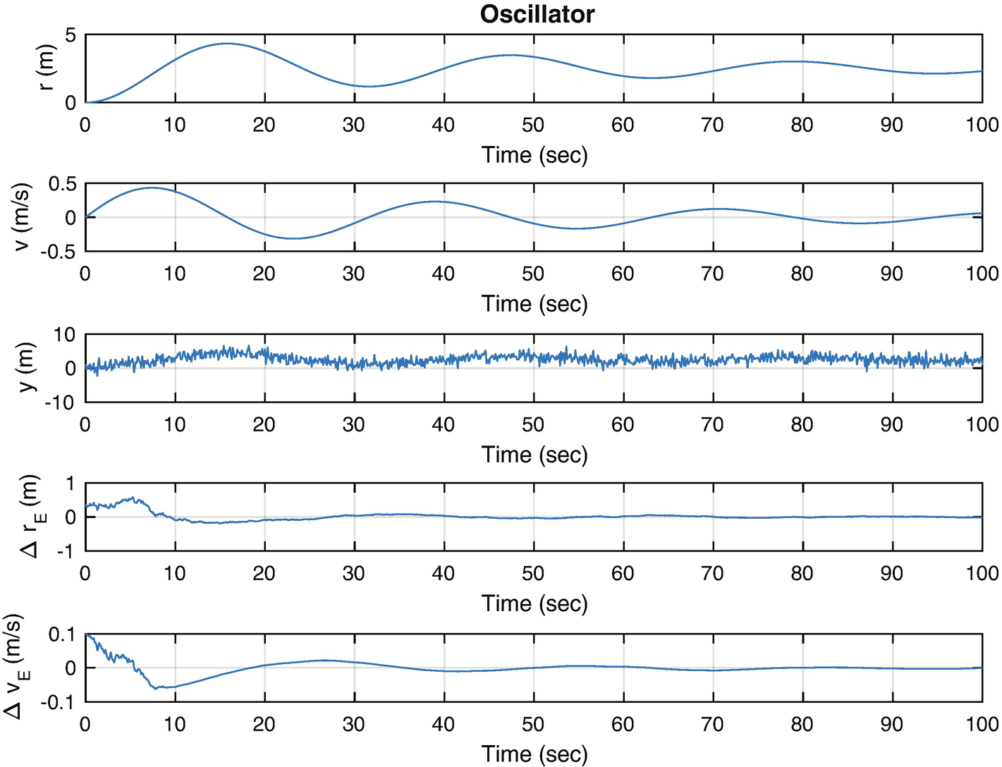
The Kalman Filter results with the higher model noise matrix, [1e-4 1e-4].

../images/420697_2_En_4_Chapter/420697_2_En_4_Fig8_HTML.png
Figure 4.8

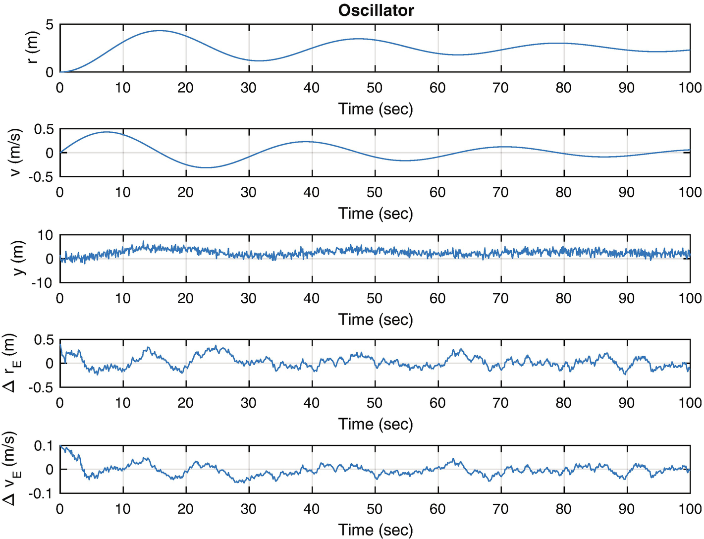
The Kalman Filter results with the lower model noise matrix, [1e-6 1e-6]. Less noise is seen but the errors are large.

4.2 Using the Extended Kalman Filter for State Estimation

4.2.1 Problem

We want to track the damped oscillator using an EKF with the nonlinear angle measurement. The EKF was developed to handle models with nonlinear dynamical models and/or nonlinear measurement models. The conventional, or linear, filter requires linear dynamical equations and linear measurements models, that is, the measurement is a linear function of the state. If the model is not linear, linear filters will not track the states very well.

Given a nonlinear model of the form:
$$\displaystyle \begin{aligned} \begin{array}{rcl} x_k &amp;\displaystyle =&amp;\displaystyle f(x_{k-1},k-1) + q_{k-1} \end{array} \end{aligned} $$
(4.80)
$$\displaystyle \begin{aligned} \begin{array}{rcl} y_k &amp;\displaystyle =&amp;\displaystyle h(x_k,k) + r_k \end{array} \end{aligned} $$
(4.81)
The prediction step is:
$$\displaystyle \begin{aligned} \begin{array}{rcl} m_k^- &amp;\displaystyle =&amp;\displaystyle f(m_{k-1},k-1) \end{array} \end{aligned} $$
(4.82)
$$\displaystyle \begin{aligned} \begin{array}{rcl} P_k^- &amp;\displaystyle =&amp;\displaystyle F_x(m_{k-1},k-1)P_{k-1} F_x(m_{k-1},k-1)^T+Q_{k-1} \end{array} \end{aligned} $$
(4.83)
F is the Jacobian of f. The update step is:
$$\displaystyle \begin{aligned} \begin{array}{rcl} v_k &amp;\displaystyle =&amp;\displaystyle y_k - h(m_k^-,k) \end{array} \end{aligned} $$
(4.84)
$$\displaystyle \begin{aligned} \begin{array}{rcl} S_k &amp;\displaystyle =&amp;\displaystyle H_x(m_k^- ,k)P_k^- H_x(m_k^- ,k)^T+R_{k} \end{array} \end{aligned} $$
(4.85)
$$\displaystyle \begin{aligned} \begin{array}{rcl} K_k &amp;\displaystyle =&amp;\displaystyle P_k^- H_x(m_k^- ,k)^TS_k^{-1} \end{array} \end{aligned} $$
(4.86)
$$\displaystyle \begin{aligned} \begin{array}{rcl} m_k &amp;\displaystyle =&amp;\displaystyle m_k^- + K_kv_k \end{array} \end{aligned} $$
(4.87)
$$\displaystyle \begin{aligned} \begin{array}{rcl} P_k&amp;\displaystyle =&amp;\displaystyle P_k^- -K_kS_kK_k^T \end{array} \end{aligned} $$
(4.88)
Fx(m, k − 1) and Hx(m, k) are the Jacobians of the nonlinear functions f and h. The Jacobians are just a matrix of partial derivatives of F and H. This results in matrices from the vectors F and H. For example, assume we have f(x, y), which is:
$$\displaystyle \begin{aligned} f = \left[ \begin{array}{l} f_x(x,y)\\ f_y(x,y) \end{array} \right] \end{aligned} $$
(4.89)
The Jacobian is
$$\displaystyle \begin{aligned} F_k = \left[ \begin{array}{rr} \frac{\partial f_x(x_k,y_k)}{\partial x}&amp;\frac{\partial f_x(x_k,y_k)}{\partial y}\\ \frac{\partial f_y(x_k,y_k)}{\partial x}&amp;\frac{\partial f_y(x_k,y_k)}{\partial y} \end{array} \right] \end{aligned} $$
(4.90)
The matrix is computed at xk, yk.

The Jacobians can be found analytically or numerically. If done numerically, the Jacobian needs to be computed about the current value of mk. In the Iterated EKF, the update step is done in a loop using updated values of mk after the first iteration. Hx(m, k) needs to be updated at each step.

4.2.2 Solution

We will use the same KFInitialize function as created in the previous recipe, but now using the ’ekf’ input. We will need functions for the derivative of the model dynamics, the measurement, and the measurement derivatives. These are implemented in RHSOscillator Partial, AngleMeasurement, and AngleMeasurementPartial.

We will also need custom versions of the filter to predict and update steps.

4.2.3 How It Works

The EKF requires a measurement function, a measurement derivative function, and a state derivative function. The state derivative function computes the a matrix:
$$\displaystyle \begin{aligned} x_{k+1} = a_k x_k \end{aligned} $$
(4.91)

You would only use the EKF if ak changed with time. In this problem, it does not. The function to compute a is RHSOscillatorPartial. It uses CToDZOH. We could have computed a once, but using CToDZOH makes the function more general.

function a = RHSOscillatorPartial( ~, ~, dT, d )
ifnargin < 1 )
   a = struct( ’zeta’,0.7071, ’omega’,0.1);
    return
end
 b = [0;1];
 a = [0 1;d.omega^2 -2*d.zeta*d.omega];
 a = CToDZOH( a, b, dT );

Our measurement is nonlinear (being an arctangent) and needs to be linearized about each value of position. AngleMeasurement computes the measurement, which is nonlinear but smooth.

 y =  atan (x(1)/d.baseline);  
AngleMeasurementPartial computes the derivative. The following function computes the c matrix
$$\displaystyle \begin{aligned} y_k = c_k x_k \end{aligned} $$
(4.92)

The partial measurement if found by taking the derivative of the arc-tangent of the angle from the baseline. The comment reminds you of this fact.

  % y = atan(x(1)/d.baseline);
 u   = x(1)/d.baseline;
 dH  = 1/(1+u^2);
 h   = [dH 0]/d.baseline;  

It is convenient that the measurement function is smooth. If there were discontinuities, the measurement partials would be difficult to compute. The EKF implementation can handle either functions for the derivatives or matrices. In the case of the functions, we use feval to call them. This can be seen in the EKFPredict and EKFUpdate functions.

EKFPredict is the state propagation step for an EKF. It numerically integrates the right-hand side using RungeKutta. RungeKutta may be overkill in some problems and a simple Euler integration may be appropriate. Euler integration is just:
$$\displaystyle \begin{aligned} x_{k+1} = x_k + \varDelta T f(x,u,t) \end{aligned} $$
(4.93)
where f(x, u, t) is the right-hand side that can be a function of the state, x, time t, and the inputs u.
function d = EKFPredict( d )
  % Get the state transition matrix
ifisempty(d.a) )
   a =  feval ( d.fX, d.m, d.t, d.dT, d.fData );
else
   a = d.a;
end
  % Propagate the mean
 d.m = RungeKutta( d.f, d.t, d.m, d.dT, d.fData );
  % Propagate the covariance
 d.p = a*d.p*a’ + d.q;  
  %% EKFUPDATE Extended Kalman Filter measurement update step.
  %% Form
  %  d = EKFUpdate( d )
  %
  %% Description
  % All inputs are after the predict state (see EKFPredict). The h
  % data field may contain either a function name for computing
  % the estimated measurements or an m by n matrix. If h is a function
  % name you must include hX which is a function to compute the m by n
  % matrix as a linearized version of the function h.
  %
  %% Inputs
  %   d   (.)  EKF data structure
  %              .m       (n,1) Mean
  %              .p       (n,n) Covariance
  %              .h       (m,n) Either a matrix or name/handle of function
  %              .hX      (*)   Name or handle of Jacobian function for h
  %              .y       (m,1) Measurement vector
  %              .r       (m,m) Measurement covariance vector
  %              .hData   (.)   Data structure for the h and hX functions
  %
  %% Outputs
  %   d   (.)  Updated EKF data structure
  %              .m       (n,1)   Mean
  %              .p       (n,n)   Covariance
  %              .v       (m,1)   Residuals
function d = EKFUpdate( d )
  % Residual
if( isnumeric( d.h ) )
   h   = d.h;
   yE  = h*d.m;
else
   h   =  feval ( d.hX, d.m, d.hData );
   yE  =  feval ( d.h,  d.m, d.hData );
end
  % Residual
 d.v     = d.y - yE;
  % Update step
 s   = h*d.p*h’ + d.r;
 k   = d.p*h’/s;
 d.m = d.m + k*d.v;
 d.p = d.p - k*s*k’;

The EKFSim script implements the EKF with all of the above functions as shown in the following listing. The functions are passed to the EKF in the data structure produced by KFInitialize. Note the use of function handles using @, i.e., @RHSOscillator. Notice that KFInitialize requires hX and fX for computing partial derivatives of the dynamical equations and measurement equations.

  %% Simulation
 xPlot =  zeros (5,nSim);
for k = 1:nSim
    % Angle measurement with random noise
   y = AngleMeasurement( x, dMeas ) + y1Sigma* randn ;
    % Update the Kalman Filter
   dKF.y = y;
   dKF   = EKFUpdate(dKF);
    % Plot storage
   xPlot(:,k) = [x;y;dKF.m-x];
    % Propagate (numerically integrate) the state equations
   x = RungeKutta( @RHSOscillator, 0, x, dT, d );
    % Propagate the Kalman Filter
   dKF = EKFPredict(dKF);
end
Figure 4.9 shows the results. The errors are small. Since the problem dynamics are linear, we don’t expect any differences from a conventional Kalman Filter.
../images/420697_2_En_4_Chapter/420697_2_En_4_Fig9_HTML.png
Figure 4.9

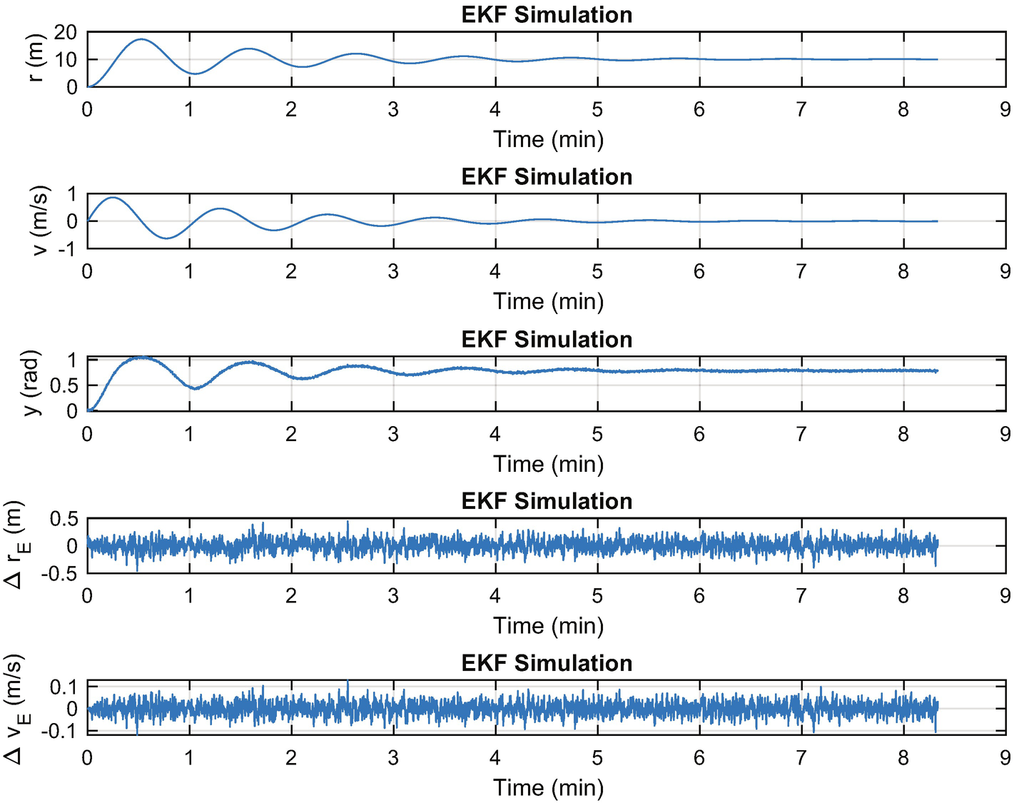
The Extended Kalman filter tracks the oscillator using the angle measurement.

4.3 Using the Unscented Kalman Filter for State Estimation

4.3.1 Problem

You want to learn the states of the spring, damper, mass system given a nonlinear angle measurement. This time we’ll use an UKF. With the UKF, we work with the nonlinear dynamical and measurement equations directly. We don’t have to linearize them as we did for the EKF with RHSOscillatorPartial and AngleMeasurementPartial. The UKF is also known as a sigma σ point filter because it simultaneously maintains models one sigma (standard deviation) from the mean.

4.3.2 Solution

We will create an UKF as a state estimator. This will absorb measurements and determine the state. It will autonomously learn about the state of the system based on a pre-existing model.

In the following text we develop the equations for the non-augmented Kalman Filter. This form only allows for additive Gaussian noise. Given a nonlinear model of the form
$$\displaystyle \begin{aligned} \begin{array}{rcl} x_k &amp;\displaystyle =&amp;\displaystyle f(x_{k-1},k-1) + q_{k-1} \end{array} \end{aligned} $$
(4.94)
$$\displaystyle \begin{aligned} \begin{array}{rcl} y_k &amp;\displaystyle =&amp;\displaystyle h(x_k,k) + r_k \end{array} \end{aligned} $$
(4.95)
Define weights as
$$\displaystyle \begin{aligned} \begin{array}{rcl} W_m^0 &amp;\displaystyle =&amp;\displaystyle \frac{\lambda}{n+\lambda} \end{array} \end{aligned} $$
(4.96)
$$\displaystyle \begin{aligned} \begin{array}{rcl} W_c^0 &amp;\displaystyle =&amp;\displaystyle \frac{\lambda}{n+\lambda} + 1 -\alpha^2 + \beta \end{array} \end{aligned} $$
(4.97)
$$\displaystyle \begin{aligned} \begin{array}{rcl} W_m^i &amp;\displaystyle =&amp;\displaystyle \frac{\lambda}{2(n+\lambda)}, i = 1,\ldots,2n \end{array} \end{aligned} $$
(4.98)
$$\displaystyle \begin{aligned} \begin{array}{rcl} W_c^i &amp;\displaystyle =&amp;\displaystyle \frac{\lambda}{2(n+\lambda)}, i = 1,\ldots,2n \end{array} \end{aligned} $$
(4.99)
m are weights on the mean state( m for mean) and c weights on the covariances. Note that $$W_m^i = W_c^i$$.
$$\displaystyle \begin{aligned} \begin{array}{rcl} \lambda = \alpha^2(n+\kappa) - n \end{array} \end{aligned} $$
(4.100)
$$\displaystyle \begin{aligned} \begin{array}{rcl} c = \lambda + n = \alpha^2(n+\kappa) \end{array} \end{aligned} $$
(4.101)
c scales the covariances to compute the sigma points, that is, the distribution of points around the mean for computing the additional states to propagate. α, β, and κ are scaling constants. General rules for the scaling constants are:
  • α – 0 for state estimation, 3 minus the number of states for parameter estimation.

  • β – Determines the spread of sigma points. Smaller means more closely spaced sigma points.

  • κ – Constant for prior knowledge. Set to 2 for Gaussian processes.

n is the order of the system. The weights can be put into matrix form:
$$\displaystyle \begin{aligned} \begin{array}{rcl} w_m &amp;=&amp; \left[W_m^0 \cdots W_m^{2n}\right]^T \end{array} \end{aligned} $$
(4.102)
$$\displaystyle \begin{aligned} \begin{array}{rcl} W &amp;=&amp; \left(I - \left[w_m \cdots w_m\right]\right) \left[ \begin{array}{ccc} W_c^0 &amp; \cdots &amp; 0\\ \vdots &amp; \ddots &amp; \vdots\\ 0 &amp; \cdots &amp; W_c^{2n} \end{array} \right] \left(I - \left[w_m \cdots w_m\right]\right)^T \end{array} \end{aligned} $$
(4.103)
I is the 2n + 1 by 2n + 1 identity matrix. In the equation vector wm is replicated 2n + 1 times. W is 2n + 1 by 2n + 1.
The prediction step is:
$$\displaystyle \begin{aligned} \begin{array}{rcl} X_{k-1} &amp;=&amp; \left[ \begin{array}{ccc} m_{k-1}&amp;\cdots&amp; m_{k-1} \end{array} \right] + \sqrt{c}\left[ \begin{array}{ccc} 0 &amp; \sqrt{P_{k-1}} &amp; -\sqrt{P_{k-1}} \end{array} \right] \end{array} \end{aligned} $$
(4.104)
$$\displaystyle \begin{aligned} \begin{array}{rcl} \hat{X}_k &amp;=&amp; f(X_{k-1},k-1) \end{array} \end{aligned} $$
(4.105)
$$\displaystyle \begin{aligned} \begin{array}{rcl} m_k^- &amp;=&amp; \hat{X}_k w_m \end{array} \end{aligned} $$
(4.106)
$$\displaystyle \begin{aligned} \begin{array}{rcl} P_k^- &amp;=&amp; \hat{X}_k W\hat{X}_k^T + Q_{k-1} \end{array} \end{aligned} $$
(4.107)
where X is a matrix where its column is the state vector possibly with an added sigma point vector. The update step is:
$$\displaystyle \begin{aligned} \begin{array}{rcl} X_k^- &amp;=&amp; \left[ \begin{array}{ccc} m_k^- &amp;\cdots&amp; m_k^- \end{array} \right] + \sqrt{c}\left[ \begin{array}{ccc} 0 &amp; \sqrt{P_k^-} &amp; -\sqrt{P_k^-} \end{array} \right] \end{array} \end{aligned} $$
(4.108)
$$\displaystyle \begin{aligned} \begin{array}{rcl} Y_k^- &amp;=&amp; h(X_k^-,k) \end{array} \end{aligned} $$
(4.109)
$$\displaystyle \begin{aligned} \begin{array}{rcl} \mu_k &amp;=&amp; Y_k^-w_m \end{array} \end{aligned} $$
(4.110)
$$\displaystyle \begin{aligned} \begin{array}{rcl} S_k &amp;=&amp; Y_k^-W[Y_k^-]^T + R_k \end{array} \end{aligned} $$
(4.111)
$$\displaystyle \begin{aligned} \begin{array}{rcl} C_k &amp;=&amp; X_k^-W[Y_k^-]^T \end{array} \end{aligned} $$
(4.112)
$$\displaystyle \begin{aligned} \begin{array}{rcl} K_k &amp;=&amp; C_k S_k^{-1} \end{array} \end{aligned} $$
(4.113)
$$\displaystyle \begin{aligned} \begin{array}{rcl} m_k &amp;=&amp; m_k^- + K_k(y_k-\mu_k) \end{array} \end{aligned} $$
(4.114)
$$\displaystyle \begin{aligned} \begin{array}{rcl} P_k &amp;=&amp; P_k^- - K_kS_kK_k^T \end{array} \end{aligned} $$
(4.115)
μk is a matrix of the measurements in which each column is a copy modified by the sigma points. Sk and Ck are intermediate quantities. The brackets around $$Y_k^-$$ are just for clarity.

4.3.3 How It Works

The weights are computed in UKFWeight.

  %% UKFWEIGHT Unscented Kalman Filter weight calculation
  %%  Form
  %   d = UKFWeight( d )
  %
  %% Description
  % Unscented Kalman Filter weights.
  %
  % The weight matrix is used by the matrix form of the Unscented
  % Transform. Both UKFPredict and UKFUpdate use the data structure
  % generated by this function.
  %
  % The constant alpha determines the spread of the sigma points around
  %   x and is usually set to between 10e-4 and 1. beta incorporates
  %   prior knowledge of the distribution of x and is 2 for a Gaussian
  %   distribution. kappa is set to 0 for state estimation and 3 -
  %   number of states for parameter estimation.
  %
  %% Inputs
  %   d   (.)       Data structure with constants
  %               .kappa (1,1)   0 for state estimation, 3-#states for
  %                               parameter estimation
  %               .m      (:,1)   Vector of mean states
  %               .alpha (1,1)   Determines spread of sigma points
  %               .beta   (1,1)   Prior knowledge - 2 for Gaussian
  %
  %% Outputs
  %  d   (.)       Data structure with constants
  %               .w      (2*n+1,2*n+1)   Weight matrix
  %               .wM     (1,2*n+1)       Weight array
  %               .wC     (2*n+1,1)       Weight array
  %               .c      (1,1)           Scaling constant
  %               .lambda (1,1)           Scaling constant
  %
function d = UKFWeight( d )
  % Compute the fundamental constants
 n           =  length (d.m);
 a2          = d.alpha^2;
 d.lambda    = a2*(n + d.kappa) - n;
 nL          = n + d.lambda;
 wMP         = 0.5* ones (1,2*n)/nL;
 d.wM        = [d.lambda/nL               wMP]’;
 d.wC        = [d.lambda/nL+(1-a2+d. beta ) wMP];
 d.c         =  sqrt (nL);
  % Build the matrix
 f           =  eye (2*n+1) - repmat(d.wM,1,2*n+1);
 d.w         = f* diag (d.wC)*f’;  

The prediction UKF step is shown in the following excerpt from UKFPredict.

  %% UKFPREDICT Unscented Kalman Filter measurement update step
function d = UKFPredict( d )
 pS      =  chol (d.p)’;
 nS      =  length (d.m);
 nSig    = 2*nS + 1;
 mM      = repmat(d.m,1,nSig);
 x       = mM + d.c*[ zeros (nS,1) pS -pS];
 xH      = Propagate( x, d );
 d.m     = xH*d.wM;
 d.p     = xH*d.w*xH’ + d.q;
 d.p     = 0.5*(d.p + d.p’);  % Force symmetry
  %% Propagate each sigma point state vector
function x = Propagate( x, d )
for j = 1:size(x,2)
   x(:,j) = RungeKutta( d.f, d.t, x(:,j), d.dT, d.fData );
end

UKFPredict uses RungeKutta for prediction, which is done by numerical integration. In effect, we are running a simulation of the model and just correcting the results with the next function, UKFUpdate. This gets to the core of the Kalman Filter. It is just a simulation of your model with a measurement correction step. In the case of the conventional linear Kalman Filter, we use a linear discrete time model.

The update UKF step is shown in the following listing. The update propagates the state one time step.

  %% UKFUPDATE Unscented Kalman Filter measurement update step.
function d = UKFUpdate( d )
  % Get the sigma points
 pS      = d.c* chol (d.p)’;
 nS      =  length (d.m);
 nSig    = 2*nS + 1;
 mM      = repmat(d.m,1,nSig);
 x       = mM + [ zeros (nS,1) pS -pS];
 [y, r] = Measurement( x, d );
 mu      = y*d.wM;
 s       = y*d.w*y’ + r;
 c       = x*d.w*y’;
 k       = c/s;
 d.v     = d.y - mu;
 d.m     = d.m + k*d.v;
 d.p     = d.p - k*s*k’;
  %% Measurement estimates from the sigma points
function [y, r] = Measurement( x, d )
 nSigma =  size (x,2);
  % Create the arrays
 lR  =  length (d.r);
 y   =  zeros (lR,nSigma);
 r   = d.r;
for j = 1:nSigma
   f         =  feval (d.hFun, x(:,j), d.hData );
   iR        = 1:lR;
   y(iR,j)   = f;
end

The sigma points are generated using chol. chol is Cholesky factorization and generates an approximate square root of a matrix. A true matrix square root is more computationally expensive and the results don’t really justify the penalty. The idea is to distribute the sigma points around the mean and chol works well. Here is an example that compares the two approaches:

 >> z = [1 0.2;0.2 2]
 z =
     1.0000    0.2000
     0.2000    2.0000
 >> b =  chol (z)
 b =
     1.0000    0.2000
          0    1.4000
 >> b*b
ans =
     1.0000    0.4800
          0    1.9600
 >> q =  sqrtm (z)
 q =
     0.9965    0.0830
     0.0830    1.4118
 >> q*q
ans =
     1.0000    0.2000
     0.2000    2.0000  

The square root actually produces a square root! The diagonal of b*b is close to z, which is all that is important.

The script for testing the UKF, UKFSim, is shown below. As noted earlier, we don’t need to convert the continuous time model into discrete time as we did for the Kalman Filter and EKF. Instead, we pass the filter the right-hand side of the differential equations. You must also pass it a measurement model, which can be nonlinear. You add UKFUpdate and UKFPredict function calls to the simulation loop. We start by initializing all parameters. KFInitialize takes parameter pairs, after ’ukf’ to initialize the filter. The remainder is the simulation loop and plotting. Initialization requires computation of the weighting matrices after calling KFInitialize.

  %% Initialize
 dKF  = KFInitialize(  ’ukf’, ’m’,xE, ’f’,@RHSOscillator, ’fData’,d,...
                       ’r’,y1Sigma^2, ’q’,q, ’p’,p,...
                       ’hFun’,@AngleMeasurement, ’hData’,dMeas, ’dT’,dT);
 dKF  = UKFWeight( dKF );  

We show the simulation loop here:

  %% Simulation
 xPlot =  zeros (5,nSim);
for k = 1:nSim
    % Measurements
   y = AngleMeasurement( x, dMeas ) + y1Sigma* randn ;
    % Update the Kalman Filter
   dKF.y = y;
   dKF   = UKFUpdate(dKF);
    % Plot storage
   xPlot(:,k)  = [x;y;dKF.m-x];
    % Propagate (numerically integrate) the state equations
   x = RungeKutta( @RHSOscillator, 0, x, dT, d );
    % Propagate the Kalman Filter
   dKF = UKFPredict(dKF);
end
The results are shown in Figure 4.10. The errors ΔrE and ΔvE are just noise. The measurement goes over a large angle range which would make a linear approximation problematic.
../images/420697_2_En_4_Chapter/420697_2_En_4_Fig10_HTML.png
Figure 4.10

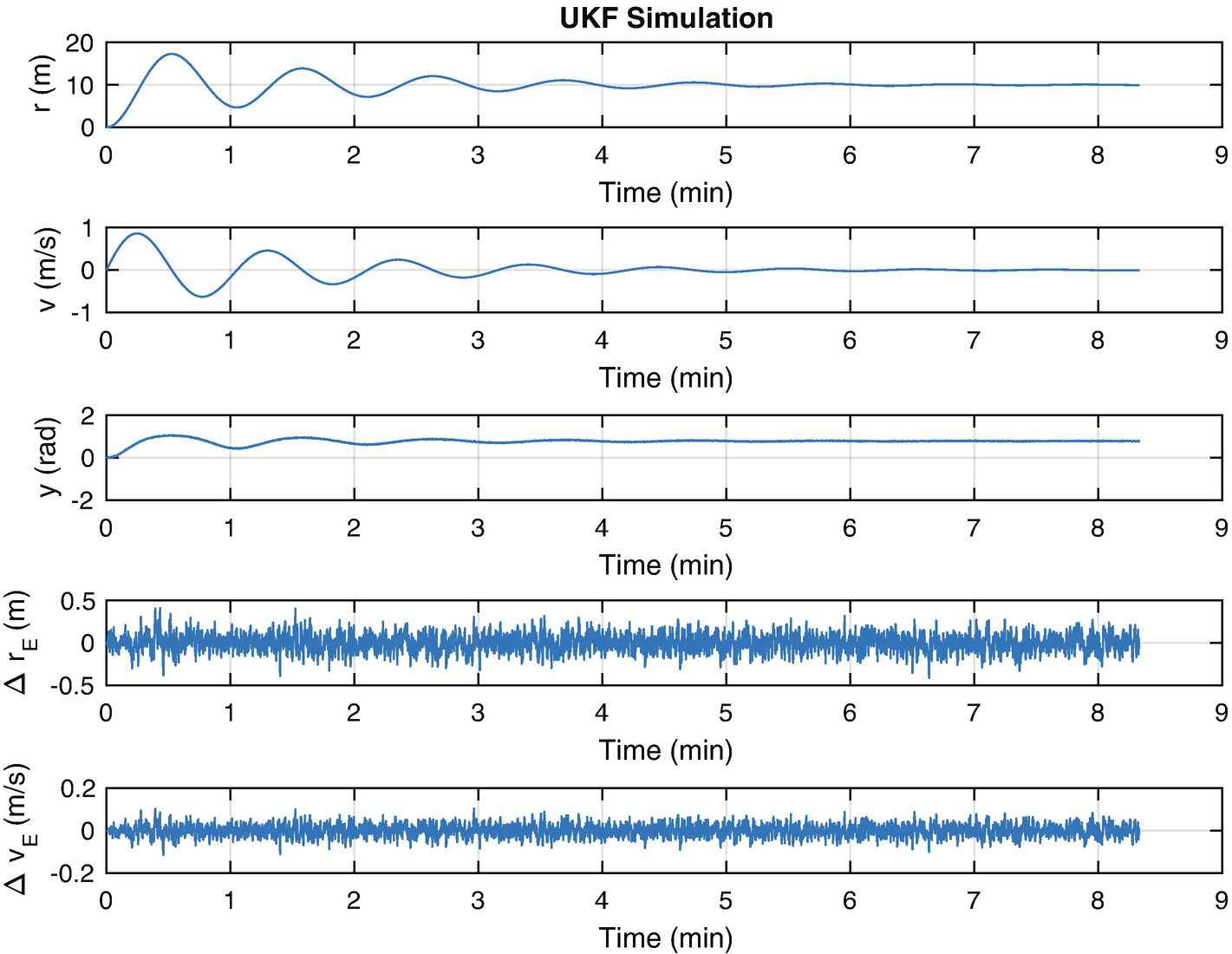
The Unscented Kalman filter results for state estimation.

4.4 Using the UKF for Parameter Estimation

4.4.1 Problem

You want to learn the parameters of the spring-damper-mass system given a nonlinear angle measurement. The UKF can be configured to do this.

4.4.2 Solution

The solution is to create a UKF configured as a parameter estimator. This will absorb measurements and determine the undamped natural frequency. It will autonomously learn about the system based on a pre-existing model. We develop the version that requires an estimate of the state that could be generated with a UKF running in parallel, as in the previous recipe.

4.4.3 How It Works

Initialize the parameter filter with the expected value of the parameters, η [28]
$$\displaystyle \begin{aligned} \hat{\eta}(t_0) = E\{\hat{\eta}_0\} \end{aligned} $$
(4.116)
and the covariance for the parameters
$$\displaystyle \begin{aligned} P_{\eta_o} = E\{(\eta(t_0) - \hat{\eta}_0)(\eta(t_0) - \hat{\eta}_0)^T\} \end{aligned} $$
(4.117)
The update sequence begins by adding the parameter model uncertainty, Q, to the covariance, P,
$$\displaystyle \begin{aligned} P = P + Q \end{aligned} $$
(4.118)
Q is for the parameters, not the states. The sigma points are then calculated. These are points found by adding the square root of the covariance matrix to the current estimate of the parameters.
$$\displaystyle \begin{aligned} \eta_{\sigma}= \left[ \begin{array}{ccc} \hat{\eta} &amp; \hat{\eta} + \gamma\sqrt{P}&amp; \hat{\eta} - \gamma\sqrt{P} \end{array} \right] \end{aligned} $$
(4.119)
γ is a factor that determines the spread of the sigma points. We use chol for the square root. If there are L parameters, the P matrix is L × L, so this array will be L × (2L + 1).
The state equations are of the form:
$$\displaystyle \begin{aligned} \dot{x} = f(x,u,t) \end{aligned} $$
(4.120)
and the measurement equations are:
$$\displaystyle \begin{aligned} y = h(x,u,t) \end{aligned} $$
(4.121)
x is the previous state of the system, as identified by the state estimator or other process. u is a structure with all other inputs to the system that are not being estimated. η is a vector of parameters that are being estimated and t is time. y is the vector of measurements. This is the dual estimation approach in that we are not estimating x and η simultaneously.

The script UKFPSim for testing the UKF parameter estimation is shown below. We are not doing the UKF state estimation to simplify the script. Normally, you would run the UKF in parallel. We start by initializing all parameters. KFInitialize takes parameter pairs to initialize the filters. The remainder is the simulation loop and plotting. Notice that there is only an update call, since parameters, unlike states, do not propagate.

for k = 1:nSim
    % Update the Kalman Filter parameter estimates
   dKF.x = x;
    % Plot storage
   xPlot(:,k) = [y;x;dKF.eta;dKF.p];
    % Propagate (numerically integrate) the state equations
   x = RungeKutta( @RHSOscillator, 0, x, dT, d );
    % Incorporate measurements
   y     = LinearMeasurement( x ) + y1Sigma* randn ;
   dKF.y = y;
   dKF   = UKFPUpdate(dKF);
end

The UKF parameter update function is shown in the following code. It uses the state estimate generated by the UKF. As noted, we are using the exact value of the state generated by the simulation. This function needs a specialized right-hand side that uses the parameter estimate, d.eta. We modified RHSOscillator for this purpose and wrote RHSOscillatorUKF.

function d = UKFPUpdate( d )
 d.wA  =  zeros (d.L,d.n);
 D     =  zeros (d.lY,d.n);
 yD    =  zeros (d.lY,1);
  % Update the covariance
 d.p = d.p + d.q;
  % Compute the sigma points
 d = SigmaPoints( d );
  % We are computing the states, then the measurements
  % for the parameters +/- 1 sigma
for k = 1:d.n
   d.fData.eta = d.wA(:,k);
   x           = RungeKutta( d.f, d.t, d.x, d.dT, d.fData );
   D(:,k)      =  feval ( d.hFun, x, d.hData );
   yD          = yD + d.wM(k)*D(:,k);
end
 pWD =  zeros (d.L,d.lY);
 pDD = d.r;
for k = 1:d.n
   wD  = D(:,k) - yD;
   pDD = pDD + d.wC(k)*(wD*wD’);
   pWD = pWD + d.wC(k)*(d.wA(:,k) - d.eta)*wD’;
end
 pDD = 0.5*(pDD + pDD’);
  % Incorporate the measurements
 K       = pWD/pDD;
 dY      = d.y - yD;
 d.eta   = d.eta + K*dY;
 d.p     = d.p - K*pDD*K’;
 d.p     = 0.5*(d.p + d.p’);  % Force symmetry
  %% Create the sigma points for the parameters
function d = SigmaPoints( d )
 n         = 2:(d.L+1);
 m         = (d.L+2):(2*d.L + 1);
 etaM      = repmat(d.eta, length (d.eta));
 sqrtP     =  chol (d.p);
 d.wA(:,1) = d.eta;
 d.wA(:,n) = etaM + d. gamma *sqrtP;
 d.wA(:,m) = etaM - d. gamma *sqrtP;  

It also has its own weight initialization function UKFPWeight.m. The weight matrix is used by the matrix form of the Unscented Transform. The constant alpha determines the spread of the sigma points around the parameter vector and is usually set to between 10e-4 and 1. beta incorporates prior knowledge of the distribution of the parameter vector and is 2 for a Gaussian distribution. kappa is set to 0 for state estimation and 3 the number of states for parameter estimation.

function d = UKFPWeight( d )
 d.L          =  length (d.eta);
 d.lambda     = d.alpha^2*(d.L + d.kappa) - d.L;
 d.gamma      =  sqrt (d.L + d.lambda);
 d.wC(1)      = d.lambda/(d.L + d.lambda) + (1 - d.alpha^2 + d. beta );
 d.wM(1)      = d.lambda/(d.L + d.lambda);
 d.n          = 2*d.L + 1;
for k = 2:d.n
   d.wC(k) = 1/(2*(d.L + d.lambda));
   d.wM(k) = d.wC(k);
end
 d.wA         =  zeros (d.L,d.n);
 y            =  feval ( d.hFun, d.x, d.hData );
 d.lY         =  length (y);
 d.D          =  zeros (d.lY,d.n);  

RHSOscillatorUKF is the oscillator model used by the UKF. It has a different input format than RHSOscillator. There is only one line of code.

 xDot = [x(2);d.a-2*d.zeta*d.eta*x(2)-d.eta^2*x(1)];  

LinearMeasurement is a simple measurement function for demonstration purposes. The UKF can use arbitrarily complex measurement functions.

The results of a simulation of an undamped oscillator are shown in Figure 4.11. The filter rapidly estimates the undamped natural frequency. The result is noisy, however. You can explore this script by varying the numbers in the script.
../images/420697_2_En_4_Chapter/420697_2_En_4_Fig11_HTML.png
Figure 4.11

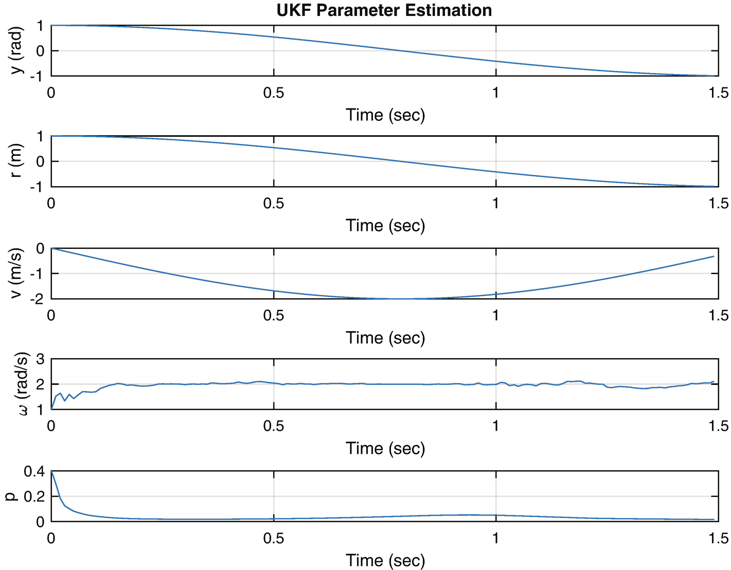
The Unscented Kalman parameter estimation results. p is the covariance. It shows that our parameter estimate has converged.

4.5 Summary

This chapter has demonstrated learning using Kalman Filters. In this case, learning is the estimation of states and parameters for a damped oscillator. We looked at conventional Kalman Filters and Unscented Kalman Filters. We looked at the parameter learning version of the latter. All examples were done using a damped oscillator. Table 4.1 lists the functions and scripts included in the companion code.
Table 4.1

Chapter Code Listing

File

Description

AngleMeasurement

Angle measurement of the mass.

AngleMeasurementPartial

Angle measurement derivative.

LinearMeasurement

Position measurement of the mass.

OscillatorSim

Simulation of the damped oscillator.

OscillatorDampingRatioSim

Simulation of the damped oscillator with different damping ratios.

RHSOscillator

Dynamical model for the damped oscillator.

RHSOscillatorPartial

Derivative model for the damped oscillator.

RungeKutta

Fourth-order Runge–Kutta integrator.

PlotSet

Create two-dimensional plots from a data set.

TimeLabel

Produce time labels and scaled time vectors.

Gaussian

Plot a Gaussian distribution.

KFInitialize

Initialize Kalman Filters.

KFSim

Demonstration of a conventional Kalman Filter.

KFPredict

Prediction step for a conventional Kalman Filter.

KFUpdate

Update step for a conventional Kalman Filter.

EKFPredict

Prediction step for an Extended Kalman Filter.

EKFUpdate

Update step for an Extended Kalman Filter.

UKFPredict

Prediction step for an Unscented Kalman Filter.

UKFUpdate

Update step for an Unscented Kalman Filter.

UKFPUpdate

Update step for an Unscented Kalman Filter parameter update.

UKFSim

Demonstration of an Unscented Kalman Filter.

UKFPSim

Demonstration of parameter estimation for the Unscented Kalman Filter.

UKFWeights

Generates weights for the Unscented Kalman Filter.

UKFPWeights

Generates weights for the Unscented Kalman Filter parameter estimator.

RHSOscillatorUKF

Dynamical model for the damped oscillator for use in Unscented Kalman Filter parameter estimation.