In this chapter, we will apply the multiple hypothesis testing (MHT) techniques from the previous chapter to the interesting problem of autonomous driving. Consider a primary car that is driving along a highway at variable speeds. It carries a radar that measures azimuth, range, and range rate. Cars pass the primary car, some of which change lanes from behind the car and cut in front. The multiple hypothesis system tracks all cars around the primary car. At the start of the simulation there are no cars in the radar field of view. One car passes and cuts in front of the radar car. The other two just pass in their lanes. You want to accurately track all cars that your radar can see.
There are two elements to this problem. One is to model the motion of the tracked automobiles using measurements to improve your estimate of each automobile’s location and velocity. The second is to systematically assign measurements to different tracks. A track should represent a single car, but the radar is just returning measurements on echoes, it doesn’t know anything about the source of the echoes.
You will solve the problem by first implementing a Kalman Filter to track one automobile. We need to write measurement and dynamics functions that will be passed to the Kalman filter, and we need a simulation to create the measurements. Then we will apply the MHT techniques developed in the previous chapter to this problem.
We’ll do the following things in this chapter.
- 1.
Model the automobile dynamics
- 2.
Model the radar system
- 3.
Write the control algorithms
- 4.
Implement visualization to let us see the maneuvers in 3D
- 5.
Implement the Unscented Kalman Filter
- 6.
Implement MHT
13.1 Automobile Dynamics
13.1.1 Problem
We need to model the car dynamics. We will limit this to a planar model in two dimensions. We are modeling the location of the car in x∕y and the angle of the wheels, which allows the car to change direction.
13.1.2 Solution
Write a right-hand side function that can be called RungeKutta.
13.1.3 How It Works
Much like with the radar, we will need two functions for the dynamics of the automobile. RHSAutomobile is used by the simulation. RHSAutomobile has the full dynamic model including the engine and steering model. Aerodynamic drag, rolling resistance and side force resistance (the car doesn’t slide sideways without resistance) are modeled. RHSAutomobile handles multiple automobiles. An alternative would be to have a one-automobile function and call RungeKutta once for each automobile. The latter approach works in all cases, except when you want to model collisions. In many types of collisions two cars collide and then stick, effectively becoming a single car. A real tracking system would need to handle this situation. Each vehicle has six states. They are:
- 1.
x position
- 2.
y position
- 3.
x velocity
- 4.
y velocity
- 5.
Angle about vertical
- 6.
Angular rate about vertical
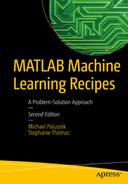
Planar automobile dynamical model.


![$$\displaystyle \begin{aligned} v= \left[ \begin{array}{l} v_x\\ v_y \end{array} \right] \end{aligned} $$](../images/420697_2_En_13_Chapter/420697_2_En_13_Chapter_TeX_Equ5.png)
![$$\displaystyle \begin{aligned} u=\frac{ \left[ \begin{array}{l} v_x\\ v_y \end{array} \right]}{\sqrt{v_x^2 + v_y^2}} \end{aligned} $$](../images/420697_2_En_13_Chapter/420697_2_En_13_Chapter_TeX_Equ6.png)
![$$\displaystyle \begin{aligned} F_{t_k}= \left[ \begin{array}{l} T/\rho - F_r\\ -F_c \end{array} \right] \end{aligned} $$](../images/420697_2_En_13_Chapter/420697_2_En_13_Chapter_TeX_Equ7.png)

 is the velocity in the tire frame in the rolling direction. For front wheel drive cars, the torque, T, is zero for the rear wheels. The contact friction is:
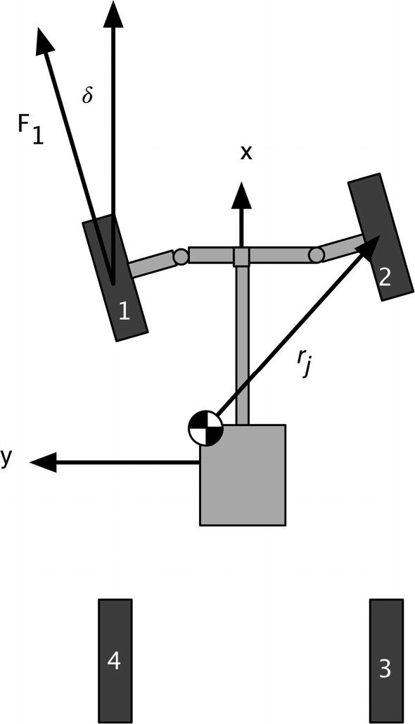
Wheel force and torque.
![$$\displaystyle \begin{aligned} c = \left[ \begin{array}{rr} \cos\delta & -\sin\delta\\ \sin\delta&\cos\delta \end{array} \right] \end{aligned} $$](../images/420697_2_En_13_Chapter/420697_2_En_13_Chapter_TeX_Equ10.png)

![$$\displaystyle \begin{aligned} v_t = c^T \left[ \begin{array}{l} v_x\\ v_y \end{array} \right] \end{aligned} $$](../images/420697_2_En_13_Chapter/420697_2_En_13_Chapter_TeX_Equ12.png)

![$$\displaystyle \begin{aligned} V = \left[ \begin{array}{rr} \cos \theta & -\sin\theta\\ \sin\theta & \cos\theta \end{array} \right]v \end{aligned} $$](../images/420697_2_En_13_Chapter/420697_2_En_13_Chapter_TeX_Equ14.png)
We’ll show you the dynamics simulation when we get to the graphics part of the chapter in Section 13.4
13.2 Modeling the Automobile Radar
13.2.1 Problem
The sensor utilized for this example will be the automobile radar. The radar measures azimuth, range, and range rate. We need two functions: one for the simulation and the second for use by the Unscented Kalman Filter.
13.2.2 Solution
Build a radar model in a MATLAB function. The function will use analytical derivations of range and range rate.
13.2.3 How It Works
The radar model is extremely simple. It assumes that the radar measures line-of-site range, range rate, and azimuth, the angle from the forward axis of the car. The model skips all the details of radar signal processing and outputs those three quantities. This type of simple model is always best when you start a project. Later on, you will need to add a very detailed model that has been verified against test data to demonstrate that your system works as expected.
 . In this model, the signal goes to zero at the maximum range that is specified in the function. The range is found from the difference in position between the radar and the target. If δ is the difference, we write:
 ![$$\displaystyle \begin{aligned} \delta = \left[ \begin{array}{l} x - x_r\\ y - y_r\\ z - z_r \end{array} \right] \end{aligned} $$](../images/420697_2_En_13_Chapter/420697_2_En_13_Chapter_TeX_Equ15.png)

![$$\displaystyle \begin{aligned} \nu = \left[ \begin{array}{l} v_x - v_{x_r}\\ v_y - v_{y_r}\\ v_z - v_{z_r} \end{array} \right] \end{aligned} $$](../images/420697_2_En_13_Chapter/420697_2_En_13_Chapter_TeX_Equ17.png)

Notice that the function has a built-in demo and, if there are no outputs, will plot the results. Adding demos to your code is a nice way to make your functions more user friendly to other people using your code and even to you when you encounter the code again several months after writing the code! We put the demo in a subfunction because it is long. If the demo is one or two lines, a subfunction isn’t necessary. Just before the demo function is the function defining the data structure.
The second function, AutoRadarUKF is the same core code, but designed to be compatible with the Unscented Kalman Filter. We could have used AutoRadar, but this is more convenient. The transformation matrix, cITOC (inertial to car transformation) is two-dimensional, since the simulation is in a flat world.
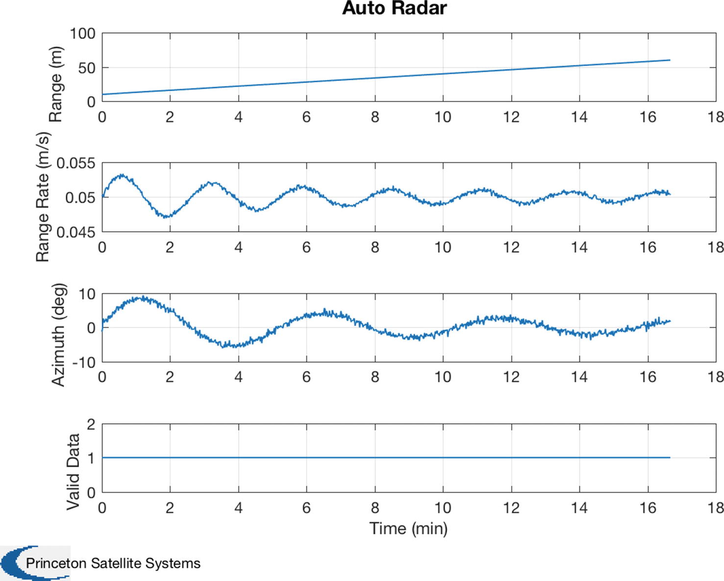
Built-in radar demo. The target is weaving in front of the radar.
13.3 Automobile Autonomous Passing Control
13.3.1 Problem
To have something interesting for our radar to measure, we need our cars to perform some maneuvers. We will develop an algorithm for a car to change lanes.
13.3.2 Solution
The cars are driven by steering controllers that execute basic automobile maneuvers. Throttle (accelerator pedal) and steering angle can be controlled. Multiple maneuvers can be chained together. This provides a challenging test for the MHT system. The first function is for autonomous passing and the second performs the lane change.
13.3.3 How It Works
The AutomobilePassing implements passing control by pointing the wheels at the target. It generates a steering angle demand and torque demand. Demand is what we want the steering to do. In a real automobile, the hardware will attempt to meet the demand, but there will be a time lag before the wheel angle or motor torque meets the wheel angle or torque demand commanded by the controller. In many cases, you are passing the demand to another control system that will try and meet the demand. The algorithms are quite simple. They don’t care if anyone gets in the way. They also don’t have any control for avoiding another vehicle. The code assumes that the lane is empty. Don’t try this with your car! The state is defined by the passState variable. Prior to passing, the passState is 0. During the passing, it is 1. When it returns to its original lane, the state is set to 0.
The second function performs a lane change. It implements lane change control by pointing the wheels at the target. The function generates a steering angle demand and a torque demand. The default gains work reasonably well. You should always supply defaults that make sense.
13.4 Automobile Animation
13.4.1 Problem
We want to visualize the cars as the maneuver.
13.4.2 How It Works
We create a function to read in .obj files. We then write a function to draw and animate the model.
13.4.3 Solution
The first part is to find an automobile model. A good resource is TurboSquid https://www.turbosquid.com. You will find thousands of models. We need .obj format and prefer a low polygon count. Ideally, we want models with triangles. In the case of the model found for this chapter, it had rectangles so we converted them to triangles using a Macintosh application, Cheetah3D https://www.cheetah3d.com. An OBJ model comes with an .obj file, an .mtl file (material file), and images for textures. We will only use the .obj file.
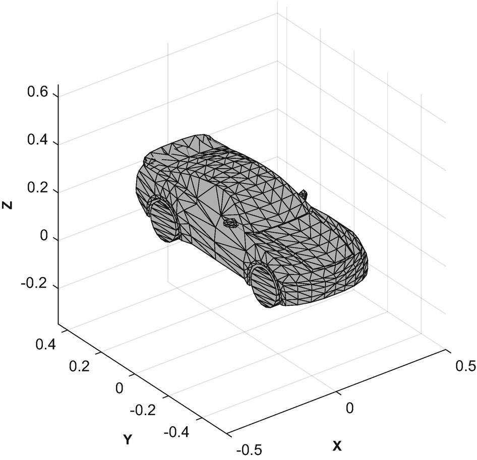
Automobile 3D model.
The image is generated with one call to patch per component.
The first part of DrawComponents initializes the model and updates it. We save, and return, pointers to the patches so that we only have to update the vectors with each call.
The mesh is drawn with a call to patch. patch has many options that are worth exploring. We use the minimal set. We make the edges black to make the model easier to see. The Phong reflection model is an empirical lighting model. It includes diffuse and specular lighting.
Updating is done by rotating the vertices around the z-axis and then adding the x and y positional offsets. The input array is [x;y;yaw]. We then set the new vertices. The function can handle an array of positions, velocities, and yaw angles.
The graphics demo AutomobileDemo implements passing control. AutomobileInitialize reads in the OBJ file. The following code sets up the graphics window:
During each pass through the simulation loop, we update the graphics. We call DrawComponents once per car along with the stored patch handles for each car’s components. We adjust the limits so that we maintain a tight focus on the two cars. We could have used the camera fields in the axes data structure for this too. We call drawnow after setting the new xlim for smooth animation.
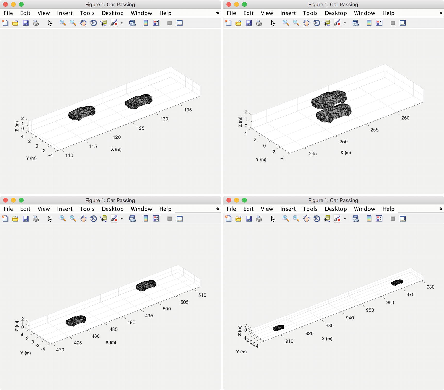
Automobile simulation snap shots showing passing.
13.5 Automobile Simulation and the Kalman Filter
13.5.1 Problem
You want to track a car using radar measurements to track an automobile maneuvering around your car. Cars may appear and disappear at any time. The radar measurement needs to be turned into the position and velocity of the tracked car. In between radar measurements you want to make your best estimate of where the automobile will be at a given time.
13.5.2 Solution
The solution is to implement an Unscented Kalman Filter to take radar measurements and update a dynamical model of the tracked automobile.
13.5.3 How It Works


The dot means time derivative or rate of change with time. These are the state equations for the automobile. This model says that the position change with time is proportional to the velocity. It also says the velocity is constant. Information about velocity changes will come solely from the measurements. We also don’t model the angle or angular rate. This is because we aren’t getting information about it from the radar. However, you may want to try including it!
The RHSAutomobileXY function is shown below; it is of only one code! This is because it just models the dynamics of the point mass.
The demonstration simulation is the same simulation used to demonstrate the multiple hypothesis system tracking. This simulation just demonstrates the Kalman Filter. Since the Kalman Filter is the core of the package, it is important that it works well before adding the measurement assignment part.
MHTDistanceUKF finds the MHT distance for use in gating computations using the Unscented Kalman Filter (UKF). The MHT distance is the distance between the observation and predicted locations. The measurement function is of the form h(x,d), where d is the UKF data structure. MHTDistanceUKF uses sigma points. The code is similar to UKFUpdate. As the uncertainty gets smaller, the residual must be smaller to remain within the gate.
The simulation UKFAutomobileDemo uses a car data structure to contain all of the car information. A MATLAB function AutomobileInitialize takes parameter pairs and builds the data structure. This is a lot cleaner than assigning the individual fields in your script. It will return a default data structure if nothing is entered as an argument.
The first part of the demo, is the automobile simulation. It generates the measurements of the automobile positions to be used by the Kalman Filter. The second part of the demo processes the measurements in the UKF to generate the estimates of the automobile track. You could move the code that generates the simulated data into a separate file if you were reusing the simulation results repeatedly.
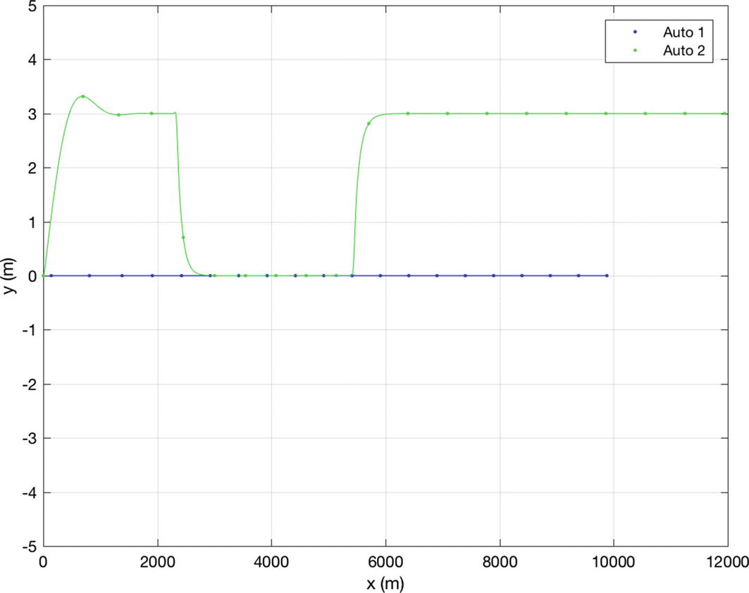
Automobile trajectories.
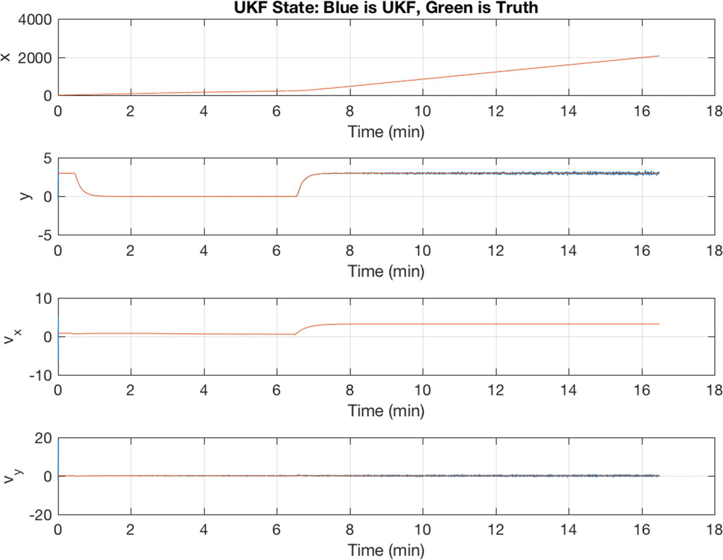
The true states and Unscented Kalman Filter (UKF) estimated states.
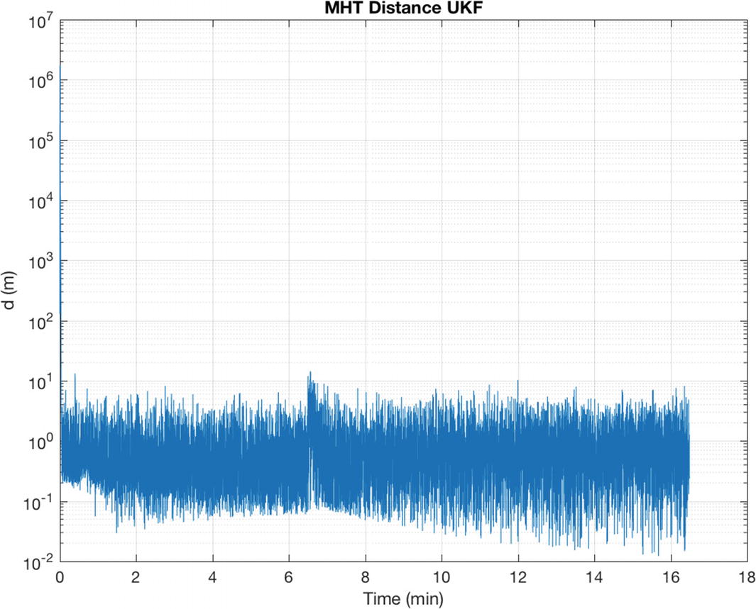
The MHT distance between the automobiles during the simulation. Notice the spike in distance when the automobile maneuver starts.
13.6 Automobile Target Tracking
13.6.1 Problem
We need to demonstrate target tracking for automobiles.
13.6.2 Solution
Build an automobile simulation with target tracking.
13.6.3 How It Works
The simulation is for a two-dimensional model of automobile dynamics. The primary car is driving along a highway at variable speeds. It carries a radar. Many cars pass the primary car, some of which change lanes from behind the car and cut in front. The MHT system tracks all cars. At the start of the simulation there are no cars in the radar field of view. One car passes and cuts in front of the radar car. The other two just pass in their lanes. This is a good test of track initiation.
The radar, covered in the first recipe of the chapter, measures range, range rate, and azimuth in the radar car frame. The model generates those values directly from the target and from the tracked cars’ relative velocity and positions. The radar signal processing is not modeled, but the radar has field-of-view and range limitations. See AutoRadar.
The cars are driven by steering controllers that execute automobile maneuvers. Throttle (accelerator pedal) and steering angle can be controlled. Multiple maneuvers can be chained together. This provides a challenging test for the MHT system. You can try different maneuvers and add additional maneuver functions of your own.
The Unscented Kalman Filter described in Chapter 4 is used in this demo as the radar is a highly nonlinear measurement. The UKF dynamical model, RHSAutomobileXY, is a pair of double integrators in the inertial frame relative to the radar car. The model accommodates steering and throttle changes by making the plant covariance, both position and velocity, larger than would be expected by analyzing the relative accelerations. An alternative would be to use interactive multiple models (IMMs) with a “steering” model and “acceleration” model. This added complication does not appear to be necessary. A considerable amount of uncertainty would be retained even with IMM, since a steering model would be limited to one or two steering angles. The script implementing the simulation with MHT is MHTAutomobileDemo. There are four cars in the demo; car 4 will be passing. Figure 13.10 shows the radar measurement for car 3, which is the last car tracked. The MHT system handles vehicle acquisition well. The MHT GUI in Figure 13.11 shows a hypothesis with three tracks at the end of the simulation. This is the expected result.
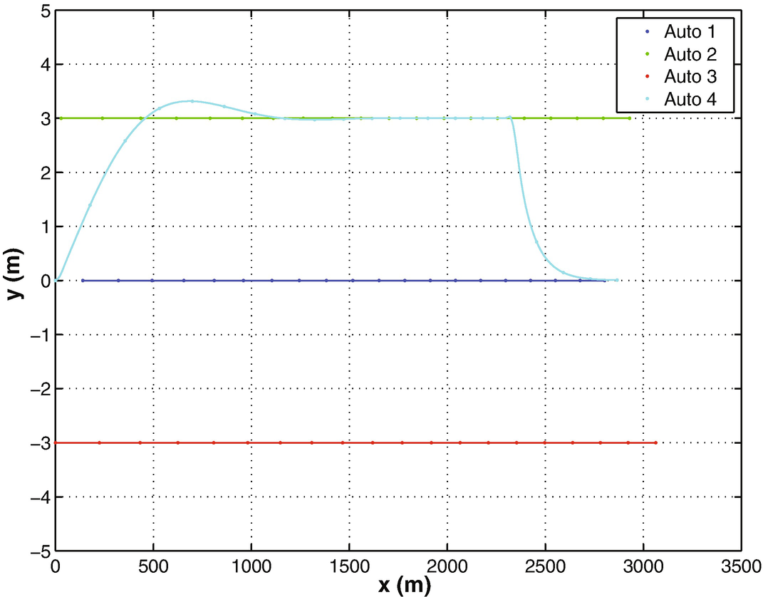
Automobile demo car trajectories.
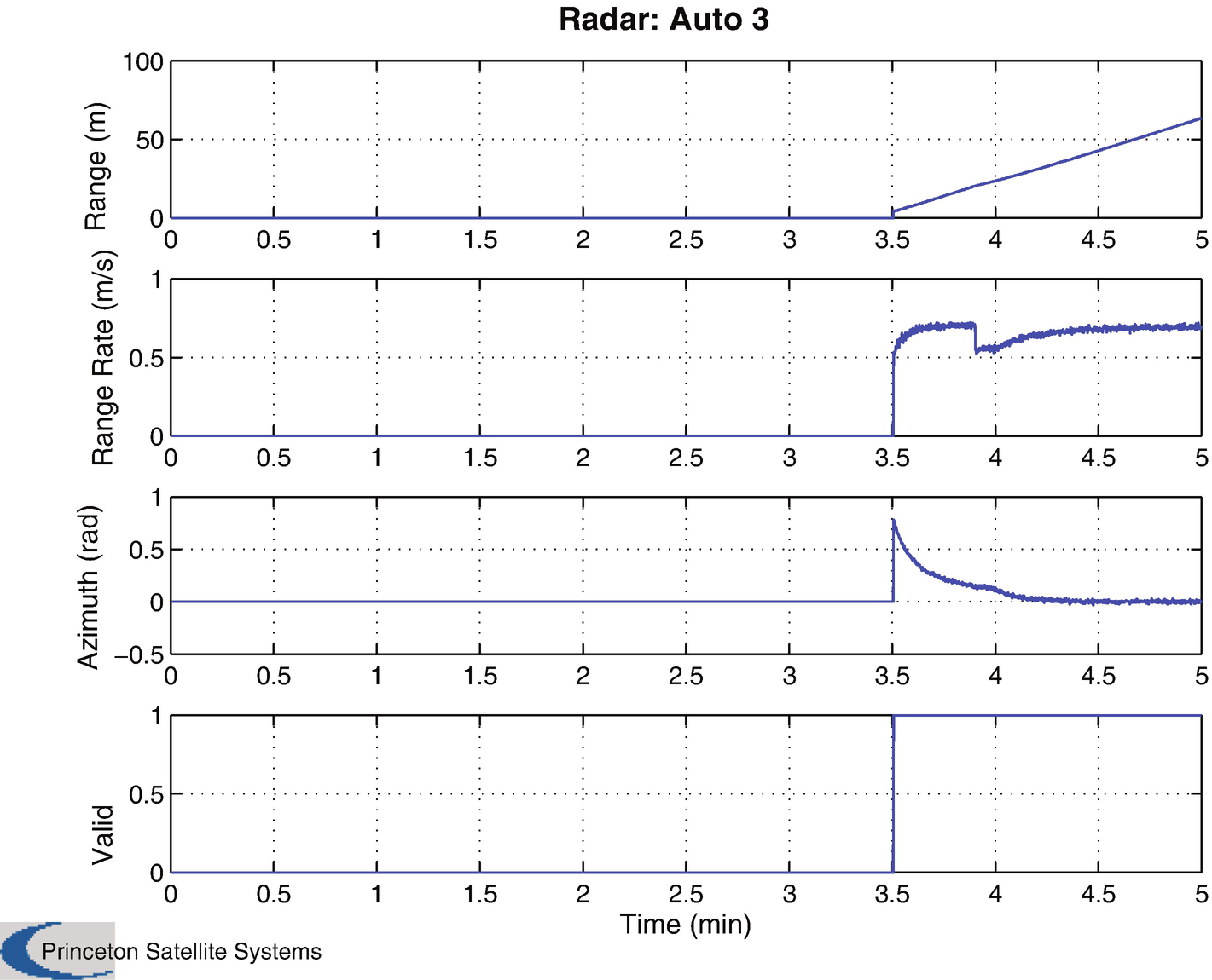
Automobile demo radar measurement for car 3.
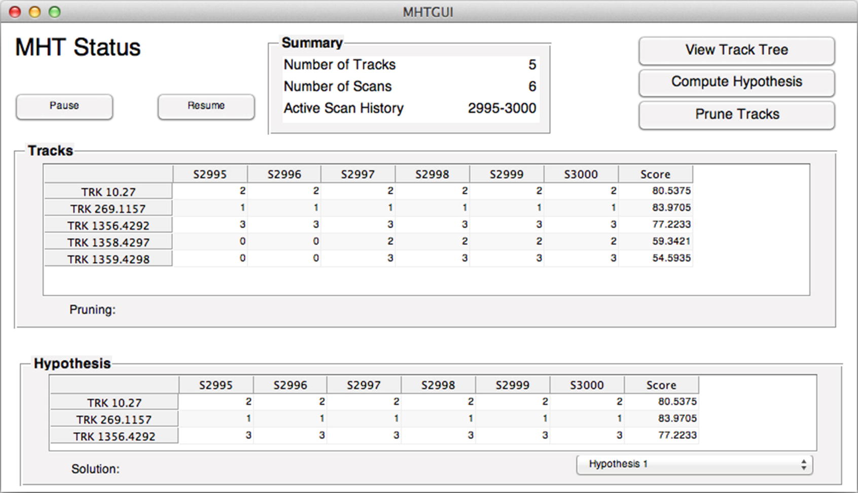
The MHT GUI shows three tracks. Each track has consistent measurements.
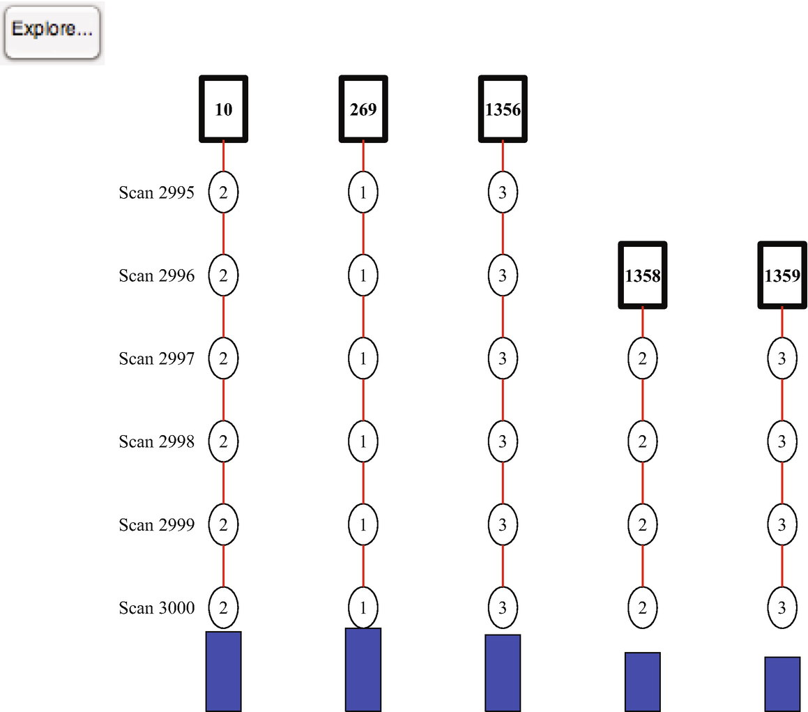
The final tree for the automobile demo.
13.7 Summary
This chapter has demonstrated an automobile tracking problem. The automobile has a radar system that detects cars in its field of view. The system accurately assigns measurements to tracks and successfully learns the path of each neighboring car. You started by building an Unscented Kalman Filter to model the motion of an automobile and to incorporate measurements from a radar system. This is demonstrated in a simulated script. You then build a script that incorporates track-oriented multiple hypothesis testing to assign measurements taken by the radar of multiple automobiles. This allows our radar system to autonomously and reliably track multiple cars.
You also learned how to make simple automobile controllers. The two controllers steer the automobiles and allow them to pass other cars.
Chapter Code Listing
File | Description |
|---|---|
AutoRadar | Automobile radar model for simulation. |
AutoRadarUKF | Automobile radar model for the UKF. |
AutomobileDemo | Demonstrate automobile animation. |
AutomobileInitialize | Initialize the automobile data structure. |
AutomobileLaneChange | Automobile control algorithm for lane changes. |
AutomobilePassing | Automobile control algorithm for passing. |
DrawComponents | Draw a 3D model. |
LoadOBJ | Load an .obj graphics file. |
MHTAutomobileDemo | Demonstrate the use of multiple hypothesis testing for automobile radar systems. |
RHSAutomobile | Automobile dynamical model for simulation. |
RHSAutomobileXY | Automobile dynamical model for the UKF. |
UKFAutomobileDemo | Demonstrate the UKF for an automobile. |