Michael Paluszek and Stephanie ThomasMATLAB Machine Learning Recipeshttps://doi.org/10.1007/978-1-4842-3916-2_8

8. Introduction to Neural Nets

Michael Paluszek¹ and Stephanie Thomas¹

(1)

Plainsboro, NJ, USA

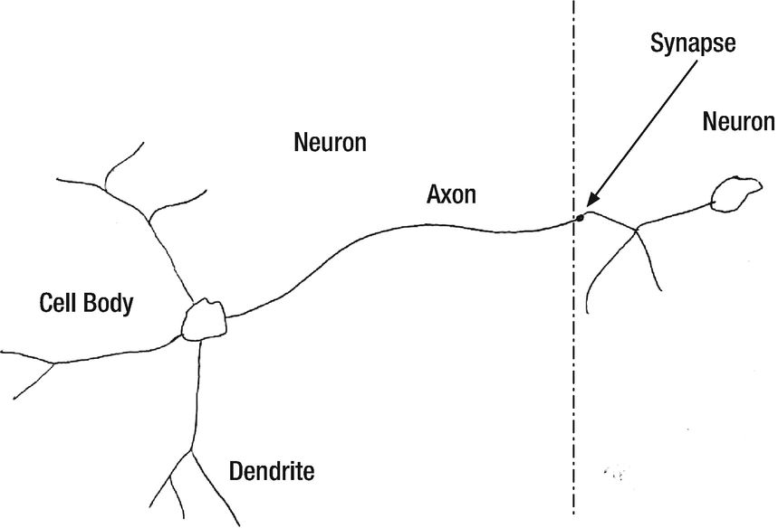
Neural networks, or neural nets, are a popular way of implementing machine “intelligence.” The idea is that they behave like the neuron in a brain. In our taxonomy, neural nets fall into the category of true machine learning, as shown on the right.

../images/420697_2_En_8_Chapter/420697_2_En_8_Figa_HTML.gif

In this chapter, we will explore how neural nets work, starting with the most fundamental idea with a single neuron and working our way up to a multi-layer neural net. Our example for this will be a pendulum. We will show how a neural net can be used to solve the prediction problem. This is one of the two uses of a neural net, prediction and categorization. We’ll start with a simple categorization example. We’ll do more sophisticated categorization neural nets in chapters 9 and 10.

8.1 Daylight Detector

8.1.1 Problem

We want to use a simple neural net to detect daylight.

8.1.2 Solution

Historically, the first neuron was the perceptron. This is a neural net with an activation function that is a threshold. Its output is either 0 or 1. This is not really useful for problems such as the pendulum angle estimation covered in the remaining recipes of this chapter. However, it is well suited to categorization problems. We will use a single perceptron in this example.

8.1.3 How It Works

Suppose our input is a light level measured by a photo cell. If you weight the input so that 1 is the value defining the brightness level at twilight, you get a sunny day detector.

This is shown in the following script, SunnyDay. The script is named after the famous neural net that was supposed to detect tanks, but instead detected sunny days; this was due to all the training photos of tanks being taken, unknowingly, on a sunny day, whereas all the photos without tanks were taken on a cloudy day. The solar flux is modeled using a cosine and scaled so that it is 1 at noon. Any value greater than 0 is daylight.

%% The data

t = linspace (0,24); % time, in hours

d = zeros (1, length (t));

s = cos ((2* pi /24)*(t-12)); % solar flux model

%% The activation function

% The nonlinear activation function which is a threshold detector

j = s < 0;

s(j) = 0;

j = s > 0;

d(j) = 1;

%% Plot the results

PlotSet(t,[s;d], ’x␣label’, ’Hour’, ’y␣label’,...

{ ’Solar␣Flux’, ’Day/Night’}, ’figure␣title’, ’Daylight␣Detector’,...

’plot␣title’, ’Daylight␣Detector’);

set([subplot(2,1,1) subplot(2,1,2)], ’xlim’,[0 24], ’xtick’,[0 6 12 18 24]);

Figure 8.1 shows the detector results. The set( gca,...) code sets the x-axis ticks to end at exactly 24 h. This is a really trivial example, but does show how categorization works. If we had multiple neurons with thresholds set to detect sun light levels within bands of solar flux, we would have a neural net sun clock.

../images/420697_2_En_8_Chapter/420697_2_En_8_Fig1_HTML.png — Figure 8.1
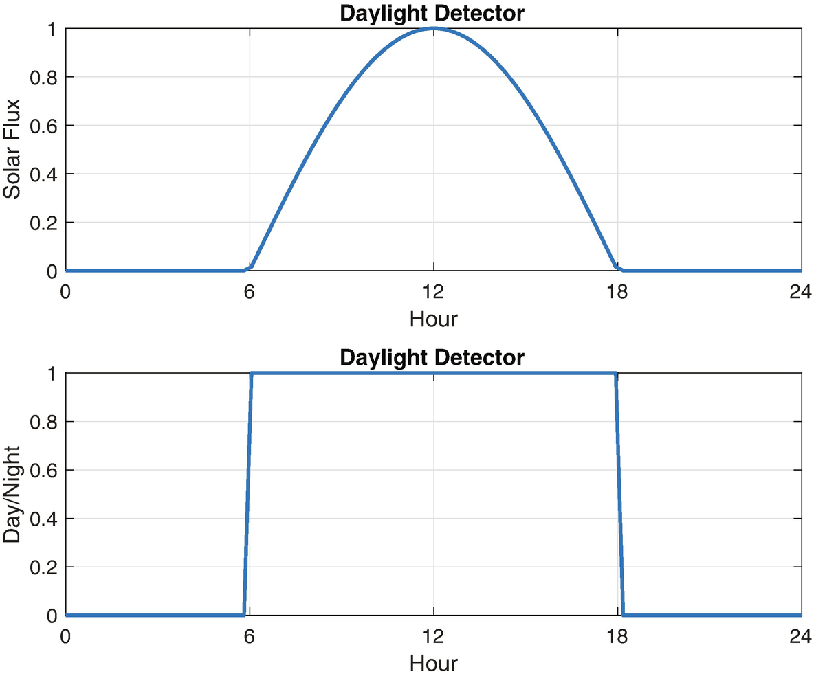
The daylight detector.

8.2 Modeling a Pendulum

8.2.1 Problem

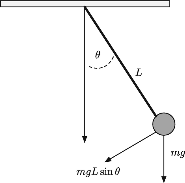
We want to implement the dynamics of a pendulum as shown in Figure 8.2. The pendulum will be modeled as a point mass with a rigid connection to its pivot. The rigid connection is a rod that cannot contract or expand.

../images/420697_2_En_8_Chapter/420697_2_En_8_Fig2_HTML.png — Figure 8.2
A pendulum. The motion is driven by the acceleration of gravity.

8.2.2 Solution

The solution is to write a pendulum dynamics function in MATLAB. The dynamics will be written in torque form, that is, we will model it as rigid body rotation. Rigid body rotation is what happens when you spin a wheel. It will use the RungeKutta integration routine in the General folder of the included toolbox to integrate the equations of motion.

8.2.3 How It Works

Figure 8.2 shows the pendulum. The easiest way to get the equations is to write it as a torque problem, that is, as rigid body rotation. When you look at a two-dimensional pendulum, it moves in a plane and its location has x and y coordinates. However, these two coordinates are constrained by the fixed pendulum of length L. We can write:

$\displaystyle \begin{aligned} L^2 = x^2 + y^2 \end{aligned}$

(8.1)

where L is the length of the rod and a constant and x and y are the coordinates in the plane. They are also the degrees of freedom in the problem. This shows that x is uniquely determined by y. If we write:

$\displaystyle \begin{aligned} \begin{array}{rcl} x&\displaystyle =&\displaystyle L\sin\theta \end{array} \end{aligned}$

(8.2)

$\displaystyle \begin{aligned} \begin{array}{rcl} y&\displaystyle =&\displaystyle L\cos\theta \end{array} \end{aligned}$

(8.3)

where θ is the angle from vertical, i.e., it is zero when the pendulum is hanging straight down, we see that we need only one degree of freedom, θ, to model the motion. So our force problem becomes a rigid body rotational motion problem. The torque is related to the angular acceleration by the inertia as:

$\displaystyle \begin{aligned} T = I\frac{d^2\theta}{dt^2} \end{aligned}$

(8.4)

where I is the inertia and T is the torque. The inertia is constant and depends on the square of the pendulum length and the mass m:

$\displaystyle \begin{aligned} I = mL^2 \end{aligned}$

(8.5)

The torque is produced by the component of the gravitational force, mg, which is perpendicular to the pendulum, where g is the acceleration of gravity. Recall that torque is the applied force, $mg\sin \theta$ , times the moment arm, in this case L. The torque is therefore:

$\displaystyle \begin{aligned} T = -mgL\sin\theta \end{aligned}$

(8.6)

The equations of motion are then:

$\displaystyle \begin{aligned} -mgL\sin\theta= mL^2\frac{d^2\theta}{dt^2} \end{aligned}$

(8.7)

or simplifying:

$\displaystyle \begin{aligned} \frac{d^2\theta}{dt^2} +\left(\frac{g}{mL}\right)\sin\theta = 0 \end{aligned}$

(8.8)

We set:

$\displaystyle \begin{aligned} \frac{g}{mL} = \varOmega^2 \end{aligned}$

(8.9)

where Ω is the frequency of the pendulum’s oscillation. This equation is nonlinear because of the $\sin \theta$ . We can linearize it about small angles, θ, about vertical. For small angles:

$\displaystyle \begin{aligned} \begin{array}{rcl} &\displaystyle &\displaystyle \sin\theta \approx \theta \end{array} \end{aligned}$

(8.10)

$\displaystyle \begin{aligned} \begin{array}{rcl} &\displaystyle &\displaystyle \cos\theta \approx 1 \end{array} \end{aligned}$

(8.11)

to get the linear constant coefficient equation. The linear version of sine comes from the Taylor’s series expansion:

$\displaystyle \begin{aligned} \sin\theta = \theta - \frac{\theta^3}{6} + \frac{\theta^5}{120} - \frac{\theta^7}{5040} + \cdots \end{aligned}$

(8.12)

You can see that the first term is a pretty good approximation around θ = 0, which is when the pendulum is hanging vertically. We can actually apply this to any angle. Let θ = θ + θ_k, where θ_k is our current angle and θ is now small. We can expand the sine term:

$\displaystyle \begin{aligned} \sin\left(\theta + \theta_k\right) = \sin\theta\cos\theta_k+\sin\theta_k\cos\theta \approx \theta\cos\theta_k + \sin\theta_k \end{aligned}$

(8.13)

We get a linear equation with a new torque term and a different coefficient for θ.

$\displaystyle \begin{aligned} \frac{d^2\theta}{dt^2} +\cos\theta_k\varOmega^2\theta = -\varOmega^2 \sin\theta_k \end{aligned}$

(8.14)

This tells us that a linear approximation may be useful, regardless of the current angle.

Our final equations (nonlinear and linear) are:

$\displaystyle \begin{aligned} \begin{array}{rcl} \frac{d^2\theta}{dt^2} + \varOmega^2\sin\theta &\displaystyle =&\displaystyle 0 \end{array} \end{aligned}$

(8.15)

$\displaystyle \begin{aligned} \begin{array}{rcl} \frac{d^2\theta}{dt^2} + \varOmega^2\theta &\displaystyle \approx&\displaystyle 0 \end{array} \end{aligned}$

(8.16)

The dynamical model is in the following code, with an excerpt from the header. This can be called by the MATLAB Recipes RungeKutta function or any MATLAB integrator. There is an option to use either the full nonlinear dynamics or the linearized form of the dynamics, using a Boolean field called linear. The state vector has the angle as the first element and the angle derivative, or angular velocity ω, as the second element. Time, the first input, is not used because it only appears in the equations as dt, so it is replaced with a tilde. The output is the derivative, xDot, of the state x. If no inputs are specified, the function will return the default data structure d.

% x (2,1) State vector [theta;theta dot]

% d (.) Data structure

% .linear (1,1) If true use a linear model

% .omega (1,1) Input gains s

function xDot = RHSPendulum( ~, x, d )

if( nargin < 1 )

xDot = struct( ’linear’,false, ’omega’,0.5);

return

end

if( d.linear )

f = x(1);

else

f = sin (x(1));

end

xDot = [x(2);-d.omega^2*f];

The code for xDot has two elements. The first element is just the second element of the state, because the derivative of the angle is the angular velocity. The second term is the angular acceleration computed using our equations. The set of differential equations that is implemented is a set of first-order differential equations:

$\displaystyle \begin{aligned} \begin{array}{rcl} \frac{d\theta}{dt} &\displaystyle =&\displaystyle \omega \end{array} \end{aligned}$

(8.17)

$\displaystyle \begin{aligned} \begin{array}{rcl} \frac{d\omega}{dt} &\displaystyle =&\displaystyle - \varOmega^2\sin\theta \end{array} \end{aligned}$

(8.18)

First order means there are only first derivatives on the left-hand side.

The script PendulumSim, shown below, simulates the pendulum by integrating the dynamical model. Setting the data structure field linear to true gives the linear model. Note that the state is initialized with a large initial angle of 3 radians to highlight the differences between the models.

%% Pendulum simulation

%% Initialize the simulation

n = 1000; % Number of time steps

dT = 0.1; % Time step (sec)

dRHS = RHSPendulum; % Get the default data structure

dRHS.linear = false; % true for linear model

%% Simulation

xPlot = zeros (2,n);

theta0 = 3; % radians

x = [theta0;0]; % [angle;velocity]

for k = 1:n

xPlot(:,k) = x;

x = RungeKutta( @RHSPendulum, 0, x, dT, dRHS );

end

%% Plot the results

yL = { ’\theta␣(rad)’ ’\omega␣(rad/s)’};

[t,tL] = TimeLabel(dT*(0:n-1));

PlotSet( t, xPlot, ’x␣label’, tL, ’y␣label’, yL, ...

’plot␣title’, ’Pendulum’, ’figure␣title’, ’Pendulum␣State’ );

Figure 8.3 shows the results of the two models. The period of the nonlinear model is not the same as that of the linear model.

../images/420697_2_En_8_Chapter/420697_2_En_8_Fig3_HTML.png — Figure 8.3
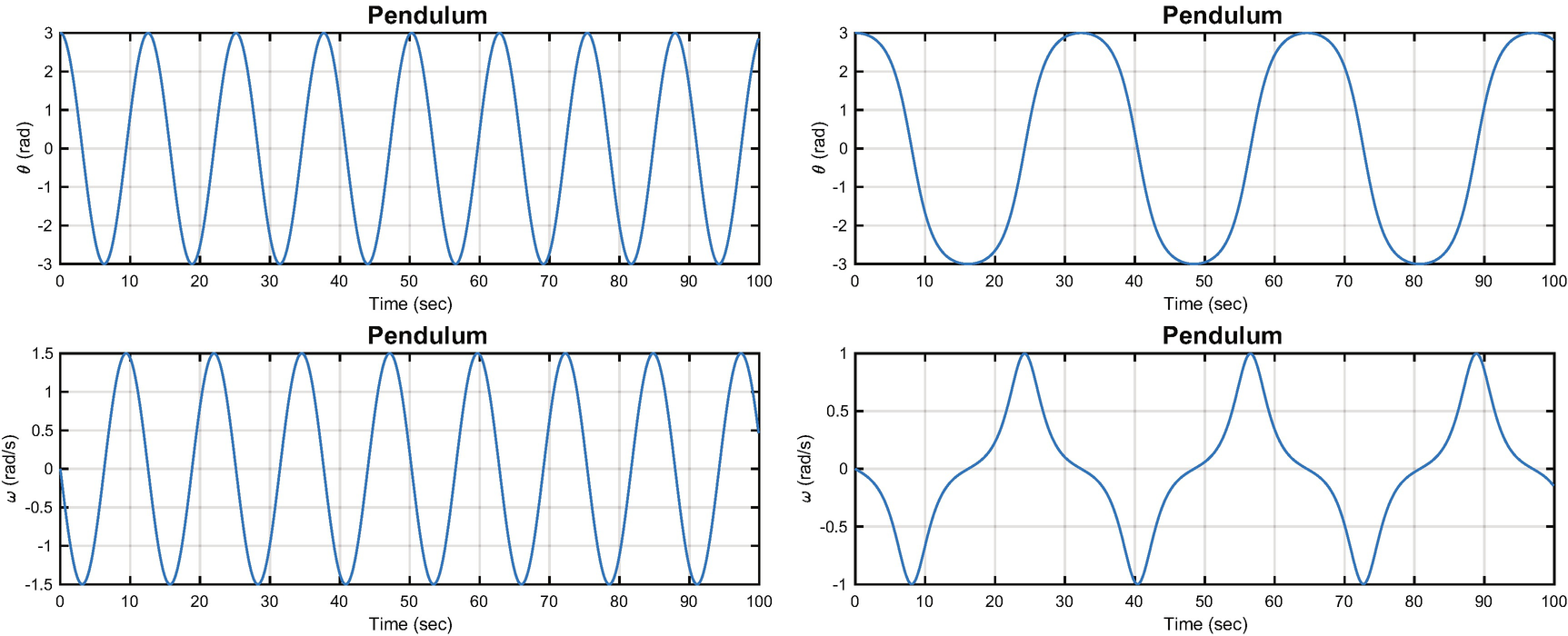
A pendulum modeled by the linear and nonlinear equations. The period for the nonlinear model is not the same as for the linear model. The left-hand plot is linear and the right nonlinear.

8.3 Single Neuron Angle Estimator

8.3.1 Problem

We want to use a simple neural net to estimate the angle between the rigid pendulum and vertical.

8.3.2 Solution

We will derive the equations for a linear estimator and then replicate it with a neural net consisting of a single neuron.

8.3.3 How It Works

Let’s first look at a single neuron with two inputs. This is shown in Figure 8.4. This neuron has inputs x ₁ and x ₂, a bias b, weights w ₁ and w ₂, and a single output z. The activation function σ takes the weighted input and produces the output.

$\displaystyle \begin{aligned} z = \sigma(w_1x_1 + w_2x_2 + b) \end{aligned}$

(8.19)

../images/420697_2_En_8_Chapter/420697_2_En_8_Fig4_HTML.png — Figure 8.4
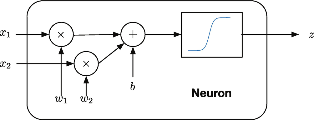
A two input neuron.

Let’s compare this with a real neuron as shown in Figure 8.5. A real neuron has multiple inputs via the dendrites. Some of these branch, which means that multiple inputs can connect to the cell body through the same dendrite. The output is via the axon. Each neuron has one output. The axon connects to a dendrite through the synapse. Signals pass from the axon to the dendrite via a synapse.

../images/420697_2_En_8_Chapter/420697_2_En_8_Fig5_HTML.png — Figure 8.5
A real neuron can have 10,000 inputs!

There are numerous commonly used activation functions. We show three:

$\displaystyle \begin{aligned} \begin{array}{rcl} \sigma(y) &\displaystyle =&\displaystyle \tanh(y) \end{array} \end{aligned}$

(8.20)

$\displaystyle \begin{aligned} \begin{array}{rcl} \sigma(y) &\displaystyle =&\displaystyle \frac{2}{1-e^{-y}} - 1 \end{array} \end{aligned}$

(8.21)

$\displaystyle \begin{aligned} \begin{array}{rcl} \sigma(y) &\displaystyle =&\displaystyle y \end{array} \end{aligned}$

(8.22)

The exponential one is normalized and offset from zero so that it ranges from -1 to 1. The following code in the script OneNeuron computes and plots these three activation functions for an input q.

%% Look at the activation functions

q = linspace (-4,4);

v1 = tanh (q);

v2 = 2./(1+ exp (-q)) - 1;

PlotSet(q,[v1;v2;q], ’x␣label’, ’Input’, ’y␣label’,...

’Output’, ’figure␣title’, ’Activation␣Functions’, ’plot␣title’, ’Activation␣Functions’,...

’plot␣set’,{[1 2 3]}, ’legend’,{{ ’Tanh’, ’Exp’, ’Linear’}});

Figure 8.6 shows the three activation functions on one plot.

../images/420697_2_En_8_Chapter/420697_2_En_8_Fig6_HTML.png — Figure 8.6
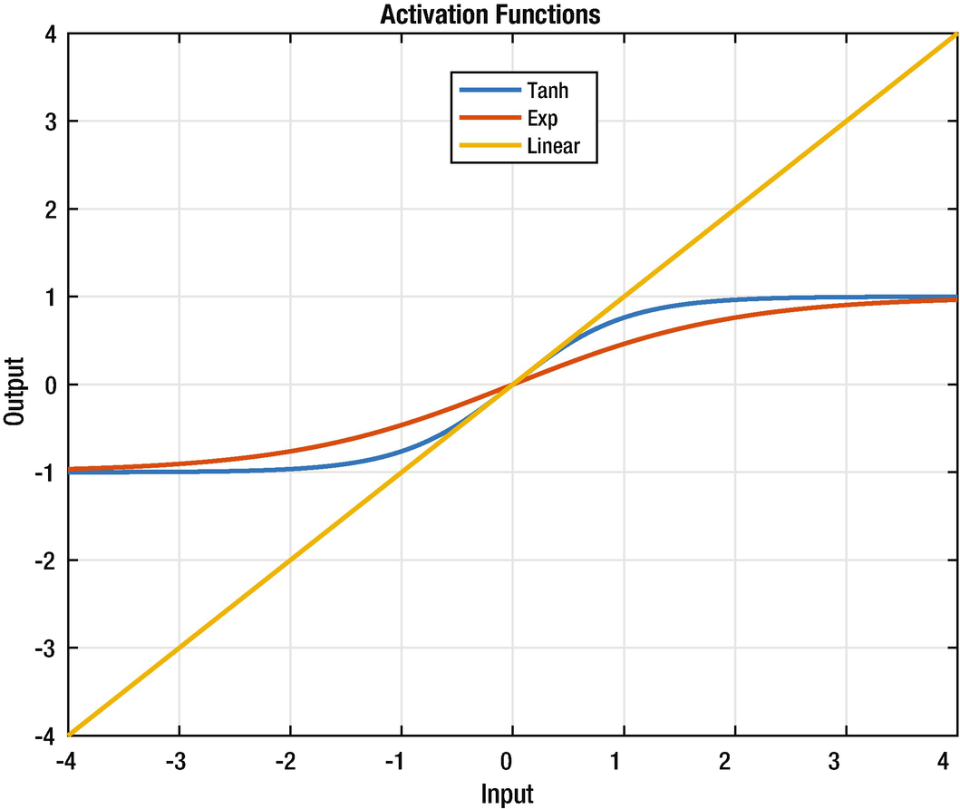
The three activation functions.

Activation functions that saturate model a biological neuron that has a maximum firing rate. These particular functions also have good numerical properties that are helpful in learning.

Now that we have defined our neuron model, let’s return to the pendulum dynamics. The solution to the linear pendulum equation is:

$\displaystyle \begin{aligned} \theta = a\sin\varOmega t + b\cos\varOmega t \end{aligned}$

(8.23)

Given the initial angle θ ₀ and angular rate $\dot {\theta }_0$ , we get the angle as a function of time:

$\displaystyle \begin{aligned} \theta(t) = \frac{\dot{\theta}_0}{\varOmega}\sin\varOmega t + \theta_0\cos\varOmega t \end{aligned}$

(8.24)

For small Ωt:

$\displaystyle \begin{aligned} \theta(t) = \dot{\theta}_0 t + \theta_0\end{aligned}$

(8.25)

which is a linear equation. Change this to a discrete time problem:

$\displaystyle \begin{aligned} \theta_{k+1} = \dot{\theta}_k \varDelta t + \theta_k\end{aligned}$

(8.26)

where Δt is the time step between measurements, θ_k is the current angle, and θ_k+1 is the angle at the next step. The linear approximation to the angular rate is:

$\displaystyle \begin{aligned} \dot{\theta}_k = \frac{\theta_k - \theta_{k-1}}{\varDelta t}\end{aligned}$

(8.27)

so combining Eqs. 8.26 and 8.27, our “estimator” is

$\displaystyle \begin{aligned} \theta_{k+1} = 2\theta_k - \theta_{k-1}\end{aligned}$

(8.28)

This is quite simple. It does not need to know the time step.

Let’s do the same thing with a neural net. Our neuron inputs are x ₁ and x ₂. If we set:

$\displaystyle \begin{aligned} \begin{array}{rcl} x_1 &\displaystyle =&\displaystyle \theta_k \end{array} \end{aligned}$

(8.29)

$\displaystyle \begin{aligned} \begin{array}{rcl} x_2 &\displaystyle =&\displaystyle \theta_{k-1} \end{array} \end{aligned}$

(8.30)

$\displaystyle \begin{aligned} \begin{array}{rcl} w_1 &\displaystyle =&\displaystyle 2 \end{array} \end{aligned}$

(8.31)

$\displaystyle \begin{aligned} \begin{array}{rcl} w_2 &\displaystyle =&\displaystyle -1 \end{array} \end{aligned}$

(8.32)

$\displaystyle \begin{aligned} \begin{array}{rcl} b &\displaystyle =&\displaystyle 0\vspace{2pt} \end{array} \end{aligned}$

(8.33)

we get

$\displaystyle \begin{aligned} z = \sigma(2\theta_k -\theta_{k-1})\end{aligned}$

(8.34)

which is, aside from the activation function σ, our estimator.

Continuing through OneNeuron, the following code implements the estimators. We input a pure sine wave that is only valid for small pendulum angles. We then compute the neuron with the linear activation function and then the tanh activation function. Note that the variable thetaN is equivalent to using the linear activation function.

%% Look at the estimator for a pendulum

omega = 1; % pendulum frequency in rad/s

t = linspace (0,20);

theta = sin (omega*t);

thetaN = 2*theta(2: end ) - theta(1: end -1); % linear estimator for "next" theta

truth = theta(3: end );

tOut = t(3: end );

thetaN = thetaN(1: end -1);

% Apply the activation function

z = tanh (thetaN);

PlotSet(tOut,[truth;thetaN;z], ’x␣label’, ’Time␣(s)’, ’y␣label’,...

’Next␣angle’, ’figure␣title’, ’One␣neuron’, ’plot␣title’, ’One␣neuron’,...

’plot␣set’,{[1 2 3]}, ’legend’,{{ ’True’, ’Estimate’, ’Neuron’}});

Figure 8.7 shows the two neuron outputs, linear and tanh, compared with the truth. The one with the linear activation function matches the truth very well. The tanh does not, but that is to be expected as it saturates.

../images/420697_2_En_8_Chapter/420697_2_En_8_Fig7_HTML.png — Figure 8.7
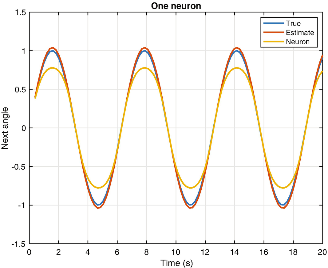
The true pendulum dynamics compared with the linear and tanh neuron output.

The one neuron function with the linear activation function is the same as the estimator by itself. Usually output nodes, and this neural net has only an output node, have linear activation functions. This makes sense, otherwise the output would be limited to the saturation value of the activation functions, as we have seen with tanh. With any other activation function, the output does not produce the desired result. This particular example is one in which a neural net doesn’t really give us any advantage and was chosen because it reduces to a simple linear estimator. For more general problems, with more inputs and nonlinear dependencies among the inputs, activation functions that have saturation may be valuable.

For this, we will need a multi-neuron net to be discussed in the last section of the chapter. Note that even the neuron with the linear activation function does not quite match the truth value. If we were to actually use the linear activation function with the nonlinear pendulum, it would not work very well. A nonlinear estimator would be complicated, but a neural net with multiple layers (deep learning) could be trained to cover a wider range of conditions.

8.4 Designing a Neural Net for the Pendulum

8.4.1 Problem

We want to estimate angles for a nonlinear pendulum.

8.4.2 Solution

We will use NeuralNetMLFF to build a neural net from training sets. (MLFF stands for multi-layer, feed-forward). We will run the net using NeuralNetMLFF. The code for NeuralNetMLFF is included with the neural net developer GUI in the next chapter.

8.4.3 How It Works

The script for this recipe is NNPendulumDemo. The first part generates the test data running the same simulation as PendulumSim.m in Recipe 8.2. We calculate the period of the pendulum in order to set the simulation time step at a small fraction of the period. Note that we will use tanh as the activation function for the net.

% Demo parameters

nSamples = 800; % Samples in the simulation

nRuns = 2000; % Number of training runs

activation = ’tanh’; % activation function

omega = 0.5; % frequency in rad/s

tau = 2* pi /omega; % period in secs

dT = tau/100; % sample at a rate of 20*omega

rng(100); % consistent random number generator

%% Initialize the simulation RHS

dRHS = RHSPendulum; % Get the default data structure

dRHS.linear = false;

dRHS.omega = omega;

%% Simulation

nSim = nSamples + 2;

x = zeros (2,nSim);

theta0 = 0.1; % starting position (angle)

x(:,1) = [theta0;0];

for k = 1:nSim-1

x(:,k+1) = RungeKutta( @RHSPendulum, 0, x(:,k), dT, dRHS );

end

The next block defines the network and trains it using NeuralNetTraining. NeuralNetTraining and NeuralNetMLFF are described in the next chapter. Briefly, we define a first layer with three neurons and a second output layer with a single neuron; the network has two inputs, which are the previous two angles.

’plot␣title’, ’Pendulum’, ’figure␣title’, ’Pendulum␣State’ );

%% Define a network with two inputs, three inner nodes, and one output

layer = struct;

layer(1,1). type = activation;

layer(1,1).alpha = 1;

layer(2,1). type = ’sum’; %’sum’;

layer(2,1).alpha = 1;

% Thresholds

layer(1,1).w0 = rand (3,1) - 0.5;

layer(2,1).w0 = rand (1,1) - 0.5;

% Weights w(i,j) from jth input to ith node

layer(1,1).w = rand (3,2) - 0.5;

layer(2,1).w = rand (1,3) - 0.5;

%% Train the network

% Order the samples using a random list

kR = ceil ( rand (1,nRuns)*nSamples);

thetaE = x(1,kR+2); % Angle to estimate

theta = [x(1,kR);x(1,kR+1)]; % Previous two angles

e = thetaE - (2*theta(1,:) - theta(2,:));

[w,e,layer] = NeuralNetTraining( theta, thetaE, layer );

PlotSet(1: length (e), e.^2, ’x␣label’, ’Sample’, ’y␣label’, ’Error^2’,...

’figure␣title’, ’Training␣Error’, ’plot␣title’, ’Training␣Error’, ’plot␣type’, ’ylog’);

% Assemble a new network with the computed weights

layerNew = struct;

layerNew(1,1). type = layer(1,1). type ;

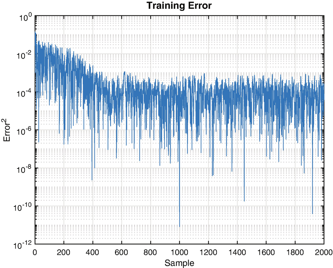
The training data structure includes the weights to be computed. It defines the number of layers and the type of activation function. The initial weights are random. Training returns the new weights and the training error. We pass the training data in a random order to the function using the index array k. This gives better results than if we passed it in the original order. We also send the same training data multiple times using the parameter nRuns. Figure 8.8 shows the training error. It looks good. To see the weights that were calculated, just display w at the command line. For example, the weights of the output node are now:

../images/420697_2_En_8_Chapter/420697_2_En_8_Fig8_HTML.png — Figure 8.8
Training error.

>> w(2)

ans =

struct with fields:

w: [-0.67518 -0.21789 -0.065903]

w0: -0.014379

type: 'tanh'

We test the neural net in the last block of code. We rerun the simulation and then run the neural net using NeuralNetMLFF. Note that you may choose to initialize the simulation with a different starting point than in the training data by changing the value of thetaD.

layerNew = struct;

layerNew(1,1). type = layer(1,1). type ;

layerNew(1,1).w = w(1).w;

layerNew(1,1).w0 = w(1).w0;

layerNew(2,1). type = layer(2,1). type ; %’sum’;

layerNew(2,1).w = w(2).w;

layerNew(2,1).w0 = w(2).w0;

network.layer = layerNew;

%% Simulate the pendulum with a different starting point

x(:,1) = [0.1;0];

%% Simulate the pendulum and test the trained network

% Choose the same or a different starting point and simulate

thetaD = 0.5;

x(:,1) = [thetaD;0];

for k = 1:nSim-1

x(:,k+1) = RungeKutta( @RHSPendulum, 0, x(:,k), dT, dRHS );

end

% Test the new network

theta = [x(1,1: end -2);x(1,2: end -1)];

thetaE = NeuralNetMLFF( theta, network );

eTSq = (x(1,3: end )-thetaE).^2;

The results in Figure 8.9 look good. The neural net estimated angle is quite close to the true angle. Note, however, that we ran exactly the same magnitude pendulum oscillation (thetaD = theta0), which is exactly what we trained it to recognize. If we run the test with a different starting point, such as 0.5 radians compared with the 0.1 of the training data, there is more error in the estimated angles, as shown in Figure 8.10.

../images/420697_2_En_8_Chapter/420697_2_En_8_Fig9_HTML.png — Figure 8.9
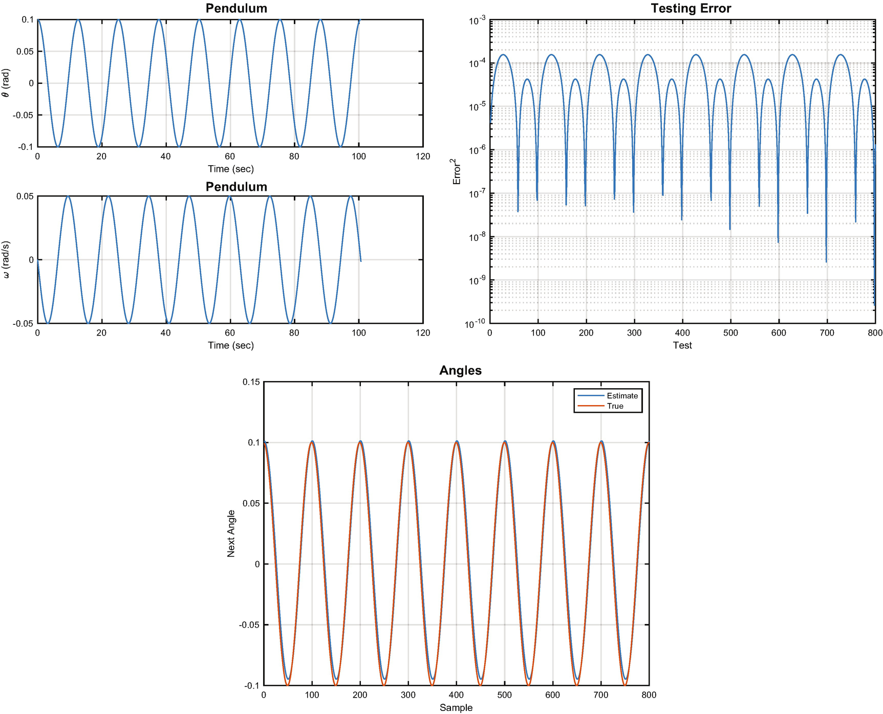
Neural net results: the simulated state, the testing error, and the truth angles compared with the neural net’s estimate.

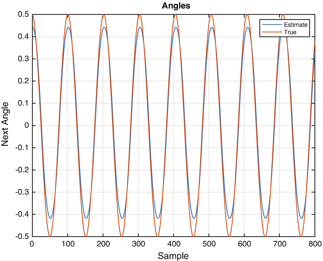
../images/420697_2_En_8_Chapter/420697_2_En_8_Fig10_HTML.png — Figure 8.10
Neural estimated angles for a different magnitude oscillation.

If we want the neural net to predict angles for other magnitudes, it needs to be trained with a diverse set of data that models all conditions. When we trained the network we let it see the same oscillation magnitude several times. This is not really productive. It might also be necessary to add more nodes to the net or more layers to make a more general purpose estimator.

8.5 Summary

This chapter has demonstrated neural learning to predict pendulum angles. It introduces the concept of a neuron. It demonstrates a one-neuron network for a pendulum and shows how it compares with a linear estimator. A perceptron example and a multi-layer pendulum angle estimator are also given. Table 8.1 lists the functions and scripts included in the companion code. The last two functions are borrowed from the next chapter, which will cover multi-layer neural nets in more depth.

Table 8.1

Chapter Code Listing

File	Description
NNPendulumDemo	Train a neural net to track a pendulum.
OneNeuron	Explore a single neuron.
PendulumSim	Simulate a pendulum.
RHSPendulum	Right-hand side of a nonlinear pendulum.
SunnyDay	Recognize daylight.
Chapter 9 Functions
NeuralNetMLFF	Compute the output of a multi-layer, feed-forward neural net.
NeuralNetTraining	Training with back propagation.