
12.1 Overview
Tracking is the process of determining the position of other objects as their position changes with time. Air traffic control radar systems are used to track aircraft. Aircraft in flight must track all nearby objects to avoid collisions and to determine if they are threats. Automobiles with radar cruise control use their radar to track cars in front of them so that the car can maintain safe spacing and avoid a collision.

When you are driving, you maintain situation awareness by identifying nearby cars and figuring out what they are going to do next. Your brain processes data from your eyes to characterize a car. You track objects by their appearance, since, in general, the cars around you all look different. Of course, at night you only have tail lights so the process is harder. You can often guess what each car is going to do, but sometimes you guess wrong and that can lead to collisions.
Radar systems just see blobs. Cameras should be able to do what your eyes and brain do, but that requires a lot of processing. As noted, at night it is hard to reliably identify a car. As the blobs are measured by radar we want to collect all blobs, as they vary in position and speed, and attach them to a particular car’s track. This way we can reliably predict where it will go next. This leads to the topic of this chapter, track-oriented multiple hypothesis testing (MHT).
Multiple Hypothesis Testing Terms
Term | Definition |
|---|---|
Clutter | Transient objects of no interest to the tracking system. |
Cluster | A collection of tracks that are linked by common observations. |
Error Ellipsoid | An ellipsoidal volume around an estimated position. |
Family | A set of tracks with a common root node. At most, one track per family can be included in a hypothesis. A family can at most represent one target. |
Gate | A region around an existing track position. Measurements within the gate are associated with the track. |
Hypothesis | A set of tracks that do not share any common observations. |
N-Scan Pruning | Using the track scores from the last N scans of data to prune tracks. The count starts from a root node. When the tracks are pruned, a new root node is established. |
Observation | A measurement that indicates the presence of an object. The observation may be of a target or be spurious. |
Pruning | Removal of low-score tracks. |
Root Node | An established track to which observations can be attached and which may spawn additional tracks. |
Scan | A set of data taken simultaneously. |
Target | An object being tracked. |
Trajectory | The path of a target. |
Track | A trajectory that is propagated. |
Track Branch | A track in a family that represents a different data association hypothesis. Only one branch can be correct. |
Track Score | The log-likelihood ratio for a track. |
Hypotheses are sets of tracks with consistent data, that is, where no measurements are assigned to more than one track. The track-oriented approach recomputes the hypotheses using the newly updated tracks after each scan of data is received. Rather than maintaining, and expanding, hypotheses from scan to scan, the track-oriented approach discards the hypotheses formed on scan k − 1. The tracks that survive pruning are propagated to the next scan k where new tracks are formed, using the new observations, and reformed into hypotheses. Except for the necessity to delete some tracks based upon low probability, no information is lost because the track scores that are maintained contain all the relevant statistical data.
The software in this chapter uses a powerful track-pruning algorithm that does the pruning in one step. Because of its speed, ad-hoc pruning methods are not required, leading to more robust and reliable results. The track management software is, as a consequence, quite simple.
The MHT Module requires the GNU Linear Programming Kit (GLPK; http://www.gnu.org/software/glpk/) and specifically, the MATLAB mex wrapper GLPKMEX (http://glpkmex.sourceforge.net). Both are distributed under the GNU license. Both the GLPK library and the GLPKMEX program are operating-system-dependent and must be compiled from the source code on your computer. Once GLPK is installed, the mex must be generated from MATLAB from the GLPKMEX source code.
The command that is executed from MATLAB to create the mex should look like:
where the “v” specifies verbose printout and you should replace /usr/local with your operating-system dependent path to your installation of GLPK. The resulting mex file (Mac) is:
The MHT software was tested with GLPK version 4.47 and GLPKMEX version 2.11.
12.2 Theory
12.2.1 Introduction
Figure 12.1 shows the general tracking problem in the context of automobile tracking. Two scans of data are shown. When the first scan is done, there are two tracks. The uncertainty ellipsoids are shown and they are based on all previous information. In the k − 1 scan (a scan is a set of measurements taken at the same time), three measurements are observed. Each scan has multiple measurements, the measurements in each new scan are numbered beginning with 1, and the measurement numbers are not meant to imply any correlation across subsequent scans. One and 3 are within the ellipsoids of the two tracks, but 2 is in both. It may be a measurement of either of the tracks or a spurious measurement. In scan k, four measurements are taken. Only measurement 4 is in one of the uncertainty ellipsoids. Three may be interpreted as spurious, but it is actually because of a new track from a third vehicle that it separates from the blue track. Measurement 1 is outside of the red ellipsoid, but is actually a good measurement of the red track and (if correctly interpreted) indicates that the model is erroneous. 4 is a good measurement of the blue track and indicates that the model is valid. Measurement 2 of scan k is outside both uncertainty ellipsoids.
- 1.
Valid
- 2.
Spurious
- 3.
A new track
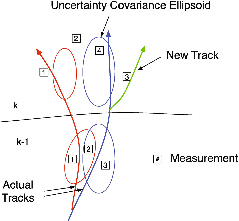
Tracking problem.
We define a contact as an observation where the signal-to-noise ratio is above a certain threshold. The observation then constitutes a measurement. Low signal-to-noise ratio observations can happen in both optical and radar systems. Thresholding reduces the number of observations that need to be associated with tracks, but may lose valid data. An alternative is to treat all observations as valid, but adjust the measurement error accordingly.
Valid measurements must then be assigned to tracks. An ideal tracking system would be able to categorize each measurement accurately and then assign them to the correct track. The system must also be able to identify new tracks and remove tracks that no longer exist. A tracking system may have to deal with hundreds of objects (perhaps after a collision or because of debris in the road).
A sophisticated system should be able to work with multiple objects as groups or clusters if the objects are more or less moving in the same direction. This reduces the number of states a system must handle. If a system handles groups, then it must be able to handle groups spawning from groups.
If we were confident that we were only tracking one vehicle, all of the data might be incorporated into the state estimate. An alternative is to incorporate only the data within the covariance ellipsoids and treat the remainders as outliers. If the latter strategy were taken, it would be sensible to remember that data in case future measurements were also “outliers,” in which case the filter might go back and incorporate different sets of outliers into the solution. This could easily happen if the model were invalid, for example, if the vehicle, which had been cruising at a constant speed, suddenly began maneuvering and the filter model did not allow for maneuvers.
The multiple model filters helps with the erroneous model problem and should be used any time a vehicle might change mode. It does not tell us how many vehicles we are tracking, however. With multiple models, each model would have its own error ellipsoids and the measurements would fit one better than the other, assuming that one of the models was a reasonable model for the tracked vehicle in its current mode.
12.2.2 Example
Referring to Figure 12.1 in the first scan, we have three measurements. 1 and 3 are associated with existing tracks and are used to update those tracks. 2 could be associated with either. It might be a spurious measurement or it could be a new track, so the algorithm forms a new hypothesis. In scan 2 measurement 4 is associated with the blue track. 1, 2, and 3 are not within the error ellipsoids of either track. Since the figure shows the true track, we can see that 1 is associated with the red track. Both 1 and 2 are just outside the error ellipsoid for the red track. Measurement 2 in scan 2 might be consistent with measurement 2 in scan 1 and could result in a new track. Measurement 3 in scan 2 is a new track, but we likely don’t have enough information to create a track until we have more scans of data.
12.2.3 Algorithm
In classical multiple target tracking, [24], the problem is divided into two steps, association and estimation. Step 1 associates contacts with targets and step 2 estimates each target’s state. Complications arise when there is more than one reasonable way to associate contacts with targets. The multiple hypothesis testing (MHT) approach is to form alternative hypotheses to explain the source of the observations. Each hypothesis assigns observations to targets or false alarms.
There are two basic approaches to MHT [3]. The first, following Reid [21], operates within a structure in which hypotheses are continually maintained and updated as observation data are received. In the second, the track-oriented approach to MHT, tracks are initiated, updated, and scored before being formed into hypotheses. The scoring process consists of comparing the likelihood that the track represents a true target versus the likelihood that it is a collation of false alarms. Thus, unlikely tracks can be deleted before the next stage, in which tracks are formed into a hypothesis. It is a good thing to discard the old hypotheses and start from scratch each time because this approach maintains the important track data while preventing an explosion of an impractically large number of hypotheses.
The track-oriented approach recomputes the hypotheses using the newly updated tracks after each scan of data is received. Rather than maintaining, and expanding, hypotheses from scan to scan, the track-oriented approach discards the hypotheses formed on scan k-1. The tracks that survive pruning are predicted to the next scan k where new tracks are formed, using the new observations, and reformed into hypotheses. Except for the necessity to delete some tracks based upon low probability or N-scan pruning, no information is lost because the track scores that are maintained contain all the relevant statistical data.
![$$\displaystyle \begin{aligned} L(K) = \log[\mathrm{LR}(K)] = \sum_{k=1}^K\left[\mathrm{LLR}_K(k) + \mathrm{LLR}_S(k)\right] + \log[L_0] \end{aligned} $$](../images/420697_2_En_12_Chapter/420697_2_En_12_Chapter_TeX_Equ1.png)

 is a natural logarithm. The likelihood ratio for the kinematic data is the probability that the data are a result of the true target divided by the probability that the data are due to a false alarm:
- 1.
M in the denominator of the third formula is the measurement dimension
- 2.
VC is the measurement volume
- 3.
S = HPTT + R the measurement residual covariance matrix
- 4.
d 2 = yTS −1y is the normalized statistical distance for the measurement
12.2.4 Measurement Assignment and Tracks
- 1.
Each measurement creates a new track.
- 2.
Each measurement in each gate updates the existing track. If there is more than one measurement in a gate, the existing track is duplicated with the new measurement.
- 3.
All existing tracks are updated with a “missed” measurement, creating a new track.
- 1.
An existing track is updated with a new measurement, assuming it corresponds to that track.
- 2.
An existing track is carried along with no update, assuming that no measurement was made for it in that scan.
- 3.
A completely new track is generated for each measurement, assuming that the measurement represents a new object.
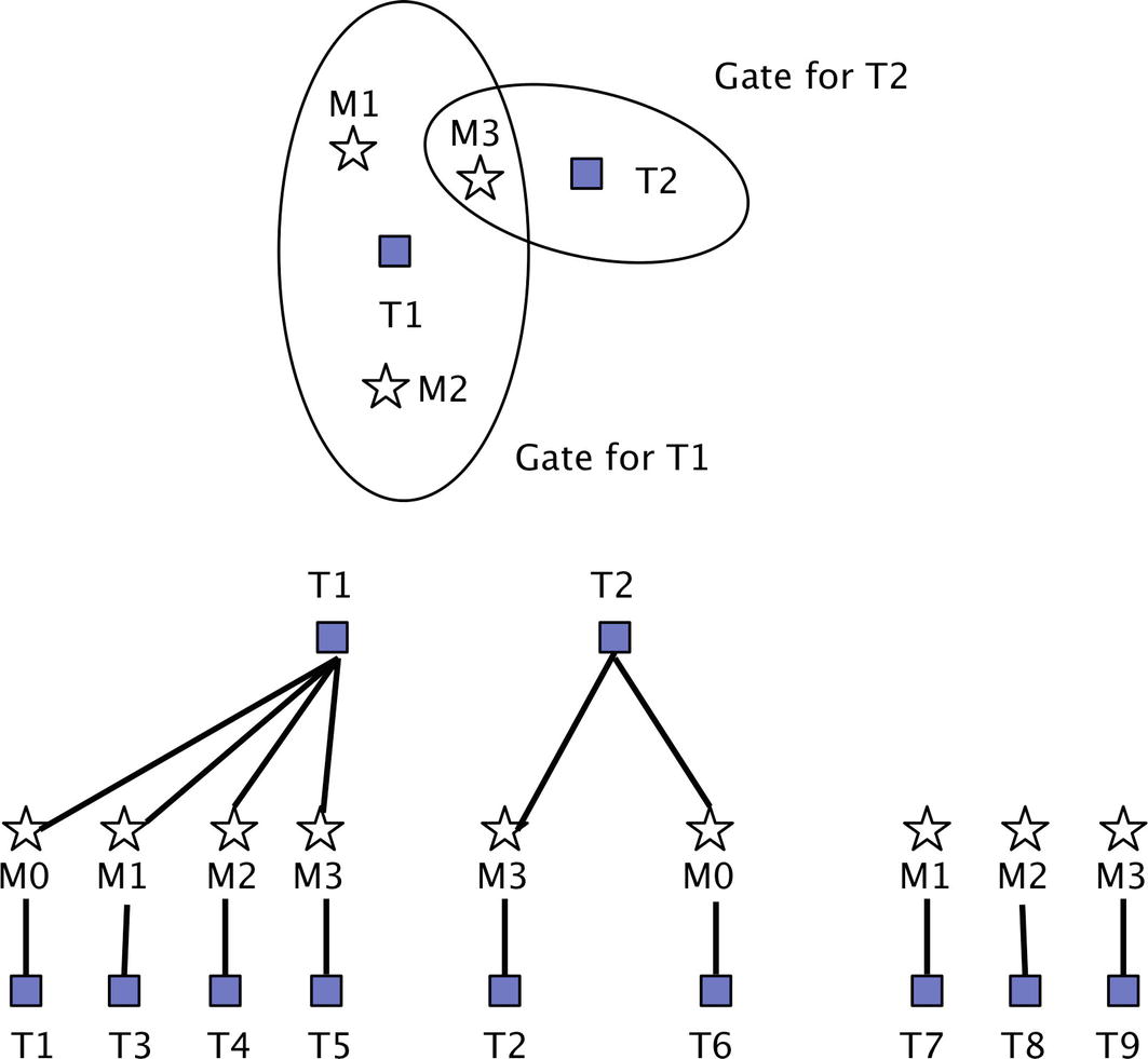
Measurement and gates. M0 is an “absent” measurement. An absent measurement is one that should exist, but does not.
12.2.5 Hypothesis Formation
In MHT, a valid hypothesis is any compatible set of tracks. In order for two or more tracks to be compatible, they cannot describe the same object, and they cannot share the same measurement at any of the scans. The task in hypothesis formation is to find one or more combinations of tracks that: 1) are compatible, and 2) maximize some performance function.
- 1.
The new track is based on some existing track, with the addition of a new measurement.
- 2.
The new track is NOT based on any existing tracks; it is based solely on a single new measurement.
Recall that each track is formed as a sequence of measurements across multiple scans. In addition to the raw measurement history, every track also contains a history of state and covariance data that is computed from a Kalman Filter. Kalman Filters are explored in Chapter 8. When a new measurement is appended to an existing track, we are spawning a new track that includes all of the original track’s measurements, plus this new measurement. Therefore, the new track is describing the same object as the original track.
A new measurement can also be used to generate a completely new track that is independent of past measurements. When this is done, we are effectively saying that the measurement does not describe any of the objects that are already being tracked. It therefore must correspond to a new/different object.
In this way, each track is given an object ID to distinguish which object it describes. Within the context of track-tree diagrams, all of the tracks inside the same track-tree have the same object ID. For example, if at some point there are 10 separate track-trees, this means that 10 separate objects are being tracked in the MHT system. When a valid hypothesis is formed, it may turn out that only a few of these objects have compatible tracks.
- 1.
No two tracks have the same object ID
- 2.
No two tracks have the same measurement index for any scan
In addition, we extend the formulation with an option to solve for multiple hypotheses, rather than just one. The algorithm will return the “M best” hypotheses, in descending order of score. This enables tracks to be preserved from alternate hypotheses that may be very close in score to the best.
12.2.6 Track Pruning
Tracks with the “N” highest scores
Tracks that are included in the “M best” hypotheses
Tracks that have both 1) the object ID and 2) the first “P” measurements found in the “M best” hypotheses.
We use the results of hypothesis formation to guide track pruning. The parameters N, M, and P can be tuned to improve performance. The objective with pruning is to reduce the number of tracks as much as possible, while not removing any tracks that should be part of the actual true hypothesis.
The second item listed above is to preserve all tracks included in the “M best” hypotheses. Each of these is a full path through a track-tree, which is clear. The third item listed above is similar, but less constrained. Consider one of the tracks in the “M best” hypotheses. We will preserve this full track. In addition, we will preserve all tracks that stem from scan “P” of this track.
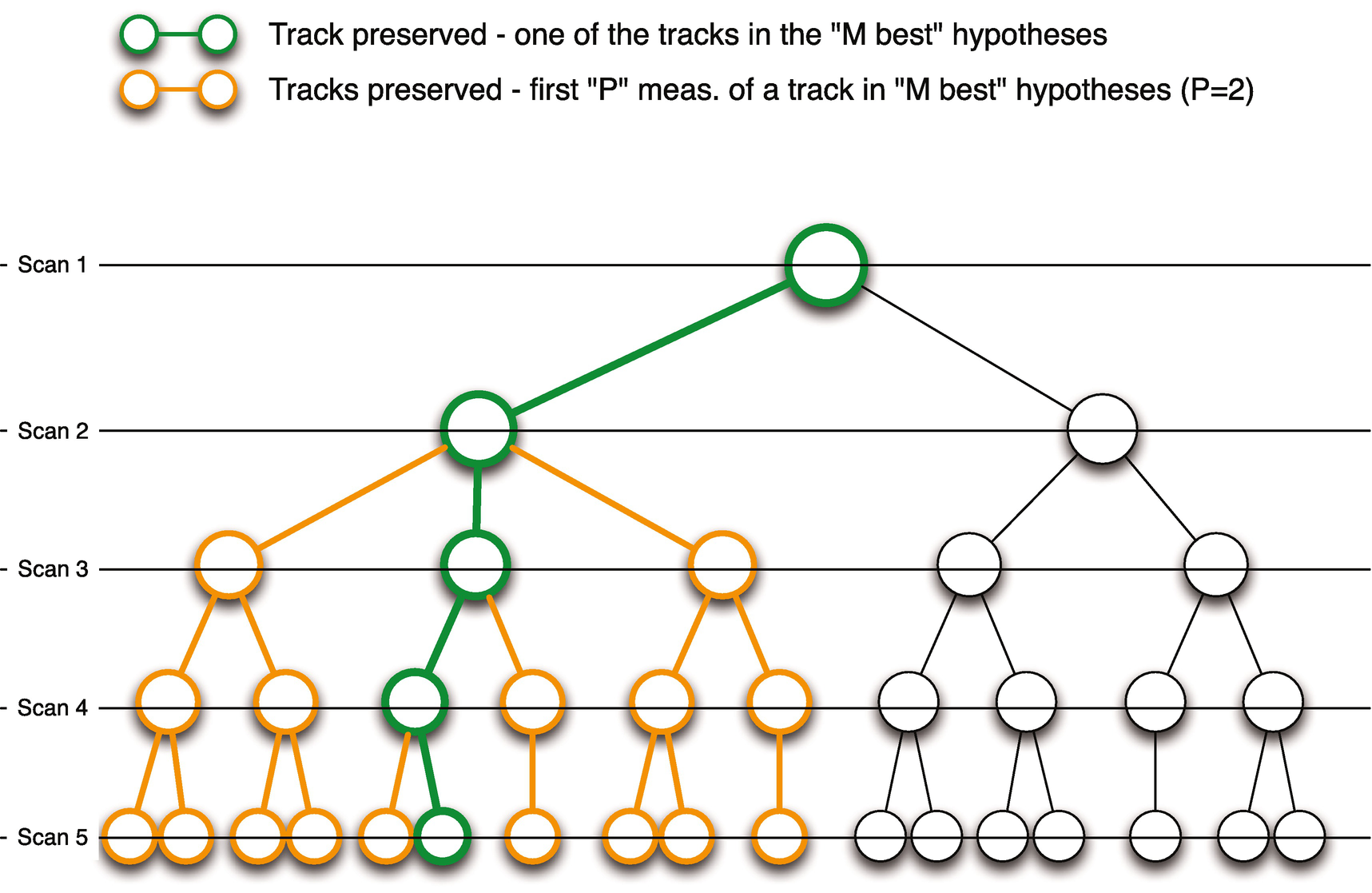
Track pruning example. This shows multiple scans (simultaneous measurements) and how they might be used to remove tracks that do not fit all of the data.
12.3 Billiard Ball Kalman Filter
12.3.1 Problem
You want to estimate the trajectory of multiple billiard balls. In the billiard ball example, we assume that we have multiple balls moving at once. Let’s say we have a video camera placed above the table, and we have software that can measure the position of each ball for each video frame. That software cannot, however, determine the identity of any ball. This is where MHT comes in. We use MHT to develop a set of tracks for the moving balls.
12.3.2 Solution
The solution is to create a linear Kalman Filter.
12.3.3 How It Works


![$$\displaystyle \begin{aligned} c = \left[\begin{array}{ll} 1 & 0 \end{array} \right] \end{aligned} $$](../images/420697_2_En_12_Chapter/420697_2_En_12_Chapter_TeX_Equ6.png)
![$$\displaystyle \begin{aligned} \begin{array}{rcl} \left[\begin{array}{l} s\\ v \end{array} \right]_{k+1} &=& \left[\begin{array}{ll} 1 & \tau\\ 0 & 1 \end{array} \right] \left[\begin{array}{l} s\\ v \end{array} \right]_k \end{array} \end{aligned} $$](../images/420697_2_En_12_Chapter/420697_2_En_12_Chapter_TeX_Equ7.png)
![$$\displaystyle \begin{aligned} \begin{array}{rcl} y_k &=& \left[\begin{array}{ll} 1 & 0 \end{array} \right] \left[\begin{array}{l} s\\ v \end{array} \right]_k \end{array} \end{aligned} $$](../images/420697_2_En_12_Chapter/420697_2_En_12_Chapter_TeX_Equ8.png)
A track, in this case, is a sequence of s. MHT assigns measurements, y to the track. If we know that we have only one object and that our sensor is measuring the track accurately, and doesn’t have any false measurements or possibility of missing measurements, we can use the Kalman Filter directly.
The KFBilliardsDemo simulates billiard balls. It includes two functions to represent the dynamics. The first is RHSBilliards, which is the right-hand-side of the billiards ball dynamics, which were just given above. This computes the position and velocity given external accelerations. The function BilliardCollision applies conservation of momentum whenever a ball hits a bumper. Balls can’t collide with other balls. The first part of the script is the simulation that generates a measurement vector for all of the balls. The second part of the script initializes one Kalman Filter per ball. This script perfectly assigns measurements to each track. The function KFPredict is the prediction step, i.e., the simulation of the ball motion. It uses the linear model described above. KFUpdate incorporates the measurements. MHTDistance is just for information purposes. The initial positions and velocity vectors of the balls are random. The script fixes the seed for the random number generator to make every run the same, which is handy for debugging. If you comment out this code each run will be different.
Here, we initialize the ball positions.
We then simulate them. Their motion is in a straight line unless they collide with a bumper.
We then process the measurements through the Kalman Filter. KFPredict predicts the next position of the balls and KFUpdate incorporates measurements. The prediction step does not know about collisions.
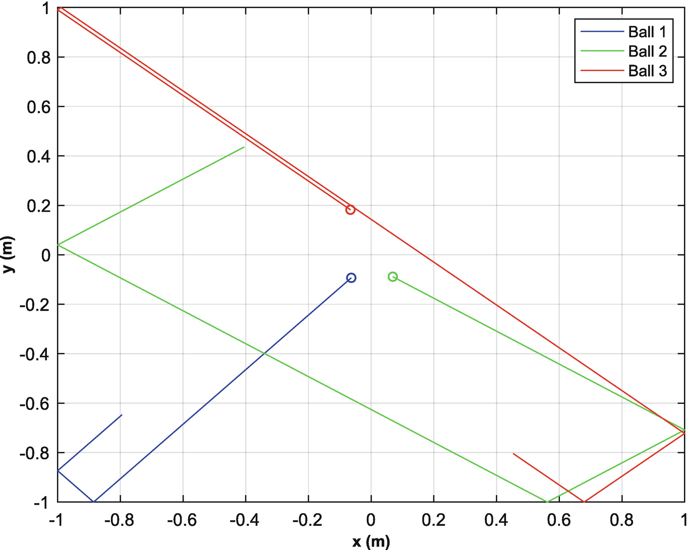
The four balls on the billiards table.
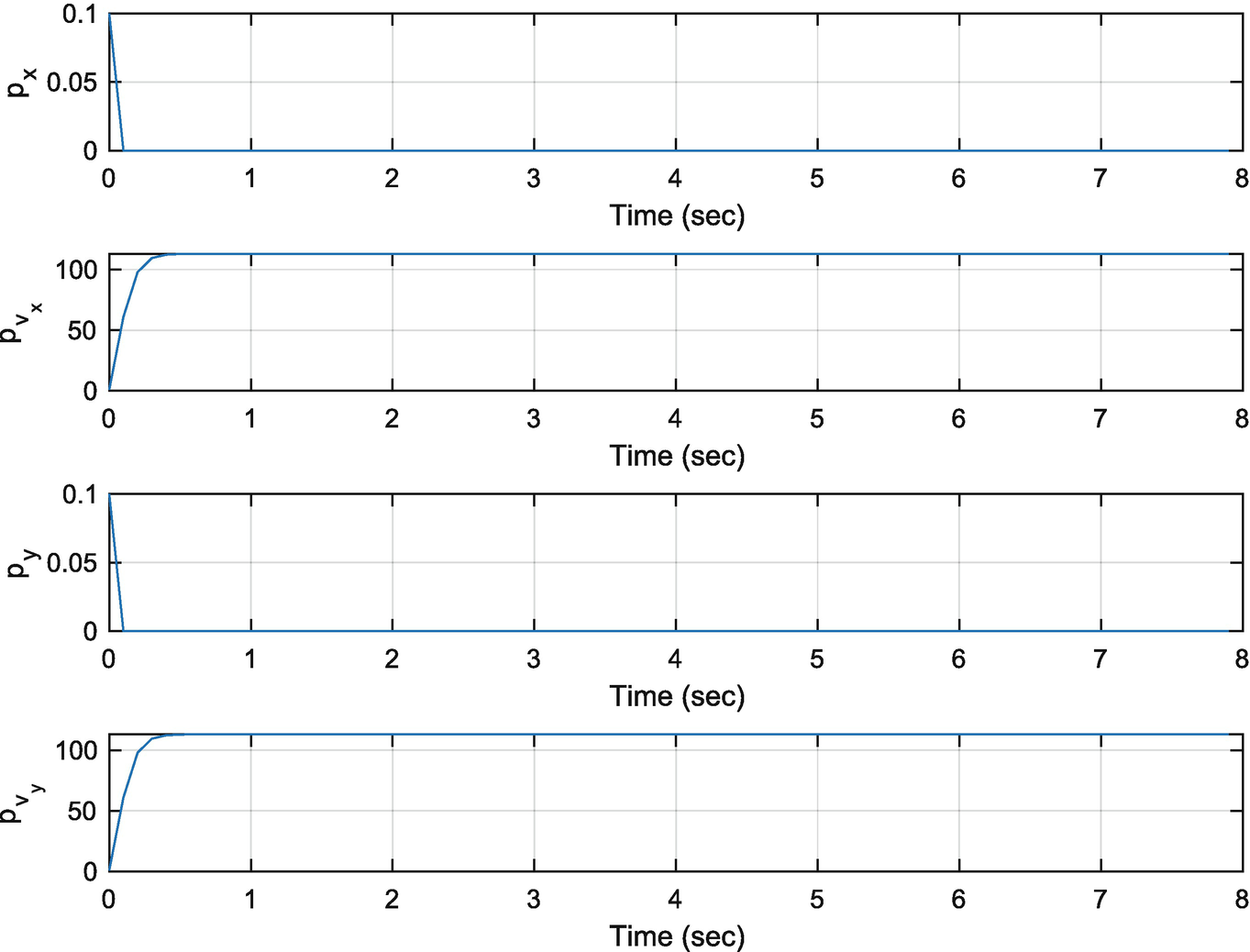
The filter covariances.
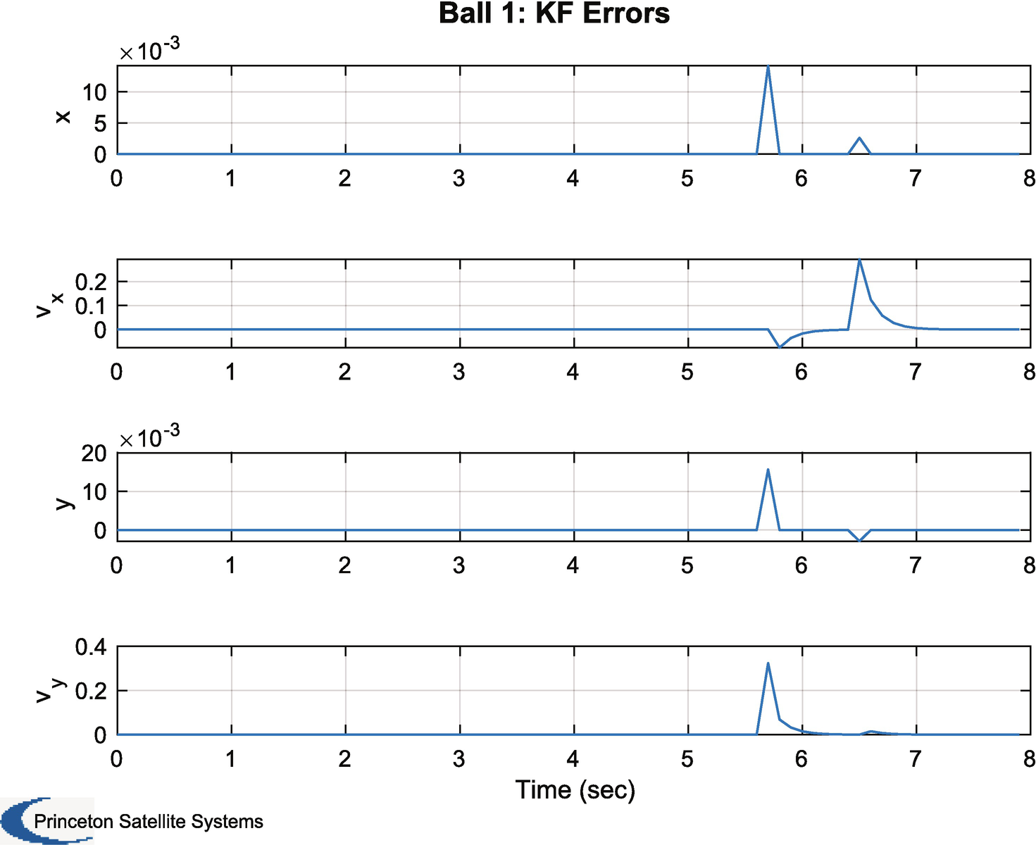
The filter errors.
The following code, excerpted from the above demo, is specialized drawing code to show the billiards on the table. It calls plot for each ball. Colors are taken from the array c and are blue, green, red, cyan, magenta, yellow, and black. You can run this from the command line once you have computed xP and yP, which are the x and y positions of the balls. The code uses the legend handles to associate the balls with the tracks in the plot in the legend. It manually sets the limits (gca as a handle to the current axes).
You can change the covariances, sigP,sigV,sigMeas in the script and see how it impacts the errors and the covariances.
12.4 Billiard Ball MHT
12.4.1 Problem
You want to estimate the trajectory of multiple billiard balls.
12.4.2 Solution
The solution is to create an MHT system with a linear Kalman Filter. This example involves billiard balls bouncing off of the bumpers of a billiard table. The model does not include the bumper collisions.
12.4.3 How It Works
The following code adds the MHT functionality. It first runs the demo, just like in the example above, and then tries to sort the measurements into tracks. It only has two balls. When you run the demo you will see the graphical user interface (GUI), Figure 12.7, and the Tree, Figure 12.8, change as the simulation progresses. We only include the MHT code in the following listing.
Multiple Hypothesis Testing Parameters
Term | Definition |
|---|---|
’probability false alarm’ | The probability that a measurement is spurious |
’probability of signal if target present’ | The probability of getting a signal if the target is present |
’probability of signal if target absent’ | The probability of getting a signal if the target is absent |
’probability of detection’ | Probability of detection of a target |
’measurement volume’ | Scales the likelihood ratio. |
’number of scans’ | The number of scans to consider in hypothesis formulation |
’gate’ | The size of the gate |
’m best’ | Number of hypotheses to consider |
’number of tracks’ | Number of tracks to maintain |
’scan to track function’ | Pointer to the scan to track function. This is custom for each application. |
’scan to track data’ | Data for the scan to track function |
’distance function’ | Pointer for the MHT distance function. Different definitions are possible. |
’hypothesis scan last’ | The last scan used in a hypothesis |
’prune tracks’ | Prune tracks if true |
’filter type’ | Type of Kalman Filter |
’filter data’ | Data for the Kalman Filter |
’remove duplicate tracks across all trees’ | If true removed duplicate tracks from all trees |
’average score history weight’ | A number to multiply the average score history |
’create track’’ | If entered it will create a track instead of using an existing track |
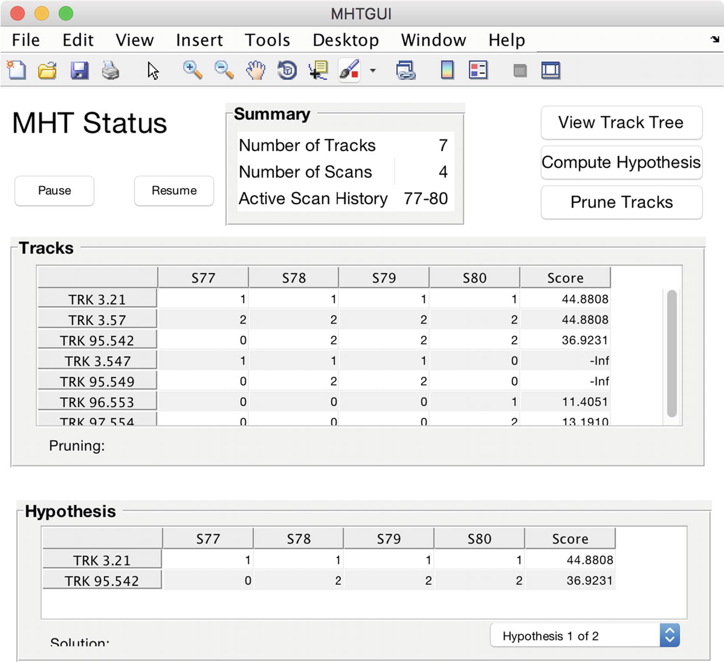
The multiple hypothesis testing (MHT) graphic user interface (GUI).
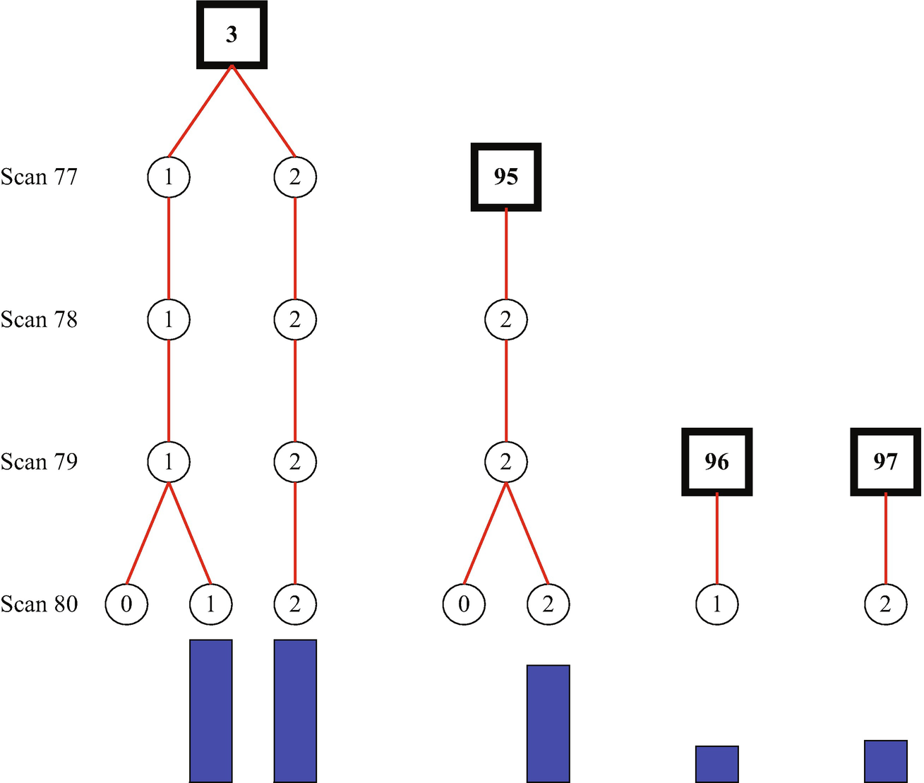
The MHT tree. The blue bars gives the score assigned to each track. Longer is better. The numbers in the framed black boxes are the track numbers.
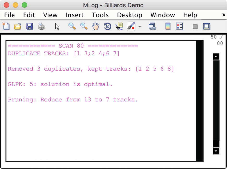
The MHT information window. It tells you what the MHT algorithm is thinking.
The demo shows that the MHT algorithm correctly associates measurements with tracks.
12.5 One-Dimensional Motion
12.5.1 Problem
You want to estimate the position of an object moving in one direction with unknown accelerations.
12.5.2 Solution
The solution is to create a linear Kalman Filter with an acceleration state.
12.5.3 How It Works
![$$\displaystyle \begin{aligned} \begin{array}{rcl} \left[\begin{array}{l} s\\ v\\ a \end{array} \right]_{k+1} &=& \left[\begin{array}{lll} 1 & \tau & \frac{1}{2}\tau^2\\ 0 & 1& \tau\\ 0 & 0 & 1 \end{array} \right] \left[\begin{array}{l} s\\ v\\ a \end{array} \right]_k \end{array} \end{aligned} $$](../images/420697_2_En_12_Chapter/420697_2_En_12_Chapter_TeX_Equ9.png)
![$$\displaystyle \begin{aligned} \begin{array}{rcl} y_k &=& \left[\begin{array}{lll} 1 & 0 & 0 \end{array} \right] \left[\begin{array}{l} s\\ v\\ a \end{array} \right]_k \end{array} \end{aligned} $$](../images/420697_2_En_12_Chapter/420697_2_En_12_Chapter_TeX_Equ10.png)
The function DoubleIntegratorWithAccel creates the matrices shown above:
with τ = 0.5 s.
We will set up the simulation so that one object has no acceleration, but starts in front of the other. The other will overtake the first. We want to see if MHT can sort out the trajectories. Passing would happen all the time with autonomous driving.
The following code implements the Kalman Filters for two vehicles. The simulation runs first to generate the measurements. The Kalman Filter runs next. Note that the plot array is updated after the filter update. This keeps it in sync with the simulation.
We use PlotSet with the argument ’plot set’ to group inputs and the argument ’legend’ to put legends on each plot. ’plot set’ takes a cell array of 1 × n arrays and ’legend’ takes a cell array of cell arrays as inputs. We don’t need to numerically integrate the equations of motion because the state equations have already done that. You can always propagate a linear model in this fashion. We set the model noise matrix using aRand, but don’t actually input any random accelerations. As written, our model is perfect, which is never true in a real system, hence the need for model uncertainty.
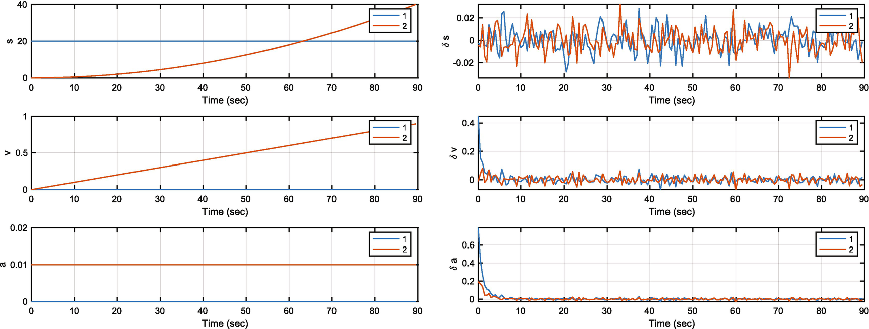
The object states and filter errors.
12.6 One-Dimensional Motion with Track Association
The next problem is one in which we need to associate measurements with a track.
12.6.1 Problem
You want to estimate the position of an object moving in one direction with measurements that need to be associated with a track.
12.6.2 Solution
The solution is to create an MHT system with the Kalman Filter as the state estimator.
12.6.3 How It Works
The MHT code is shown below. We append the MHT software to the script shown above. The Kalman Filters are embedded in the MHT software. We first run the simulation and gather the measurements and then process them in the MHT code.
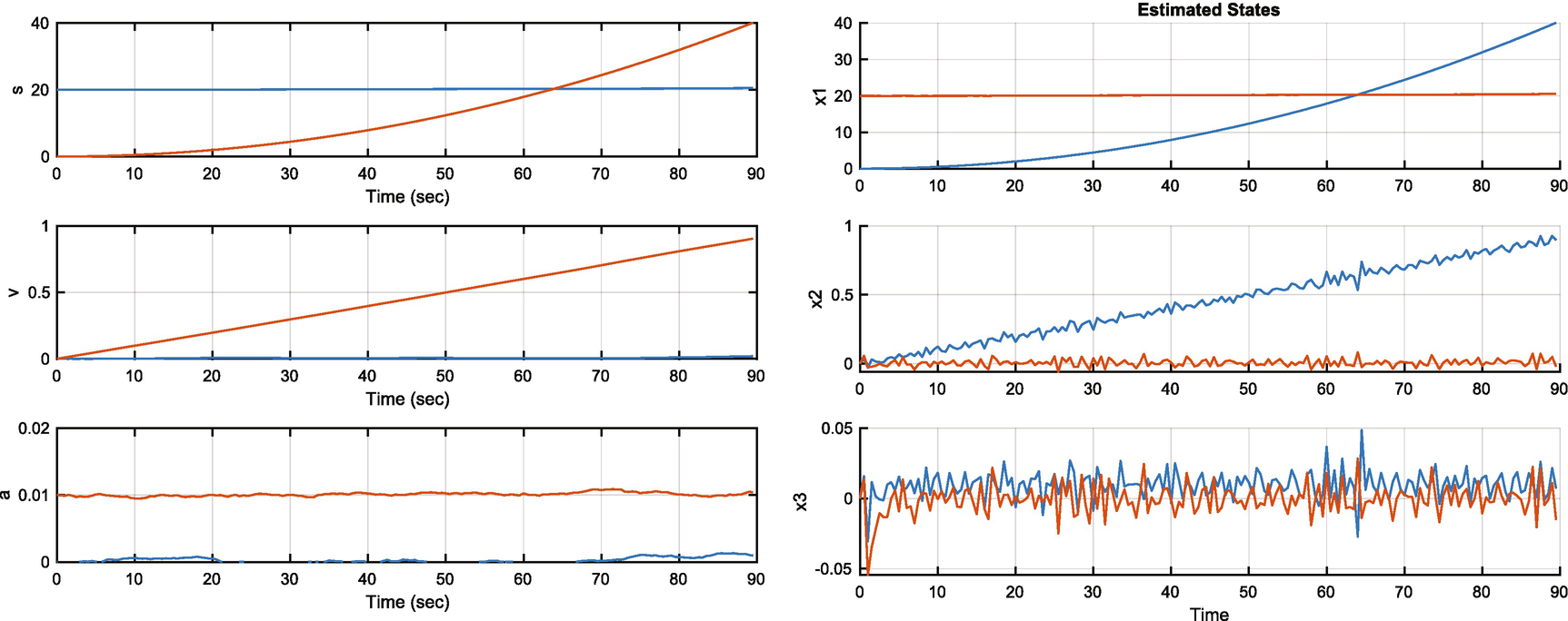
The MHT object states and estimated states. The colors are switched between plots.
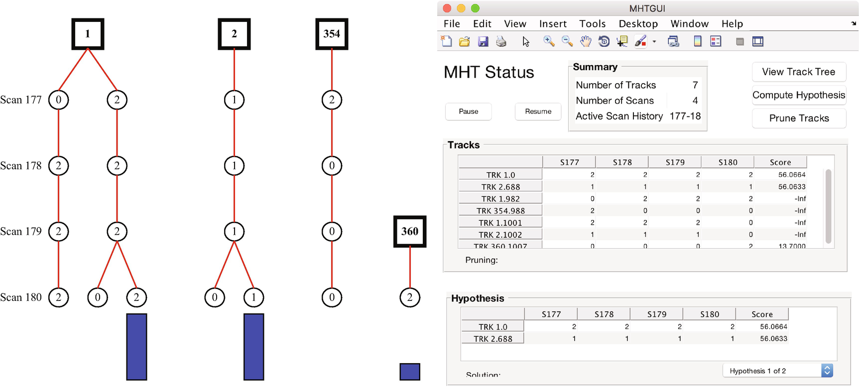
The GUI and MHT tree. The tree shows the MHT decision process.
12.7 Summary
Chapter Code Listing
File | Description |
|---|---|
AddScan | Add a scan to the data. |
CheckForDuplicateTracks | Look through the recorded tracks for duplicates. |
MHTDistanceUKF | Compute the MHT distance. |
MHTGUI.fig | Saved layout data for the MHT GUI. |
MHTGUI | GUI for the MHT software. |
MHTHypothesisDisplay | Display hypotheses in a GUI. |
MHTInitialize | Initialize the MHT algorithm. |
MHTInitializeTrk | Initialize a track. |
MHTLLRUpdate | Update the log likelihood ratio. |
MHTMatrixSortRows | Sort rows in the MHT. |
MHTMatrixTreeConvert | Convert to and from a tree format for the MHT data. |
MHTTrackMerging | Merge MHT tracks. |
MHTTrackMgmt | Manage MHT tracks. |
MHTTrackScore | Compute the total score for the track. |
MHTTrackScoreKinematic | Compute the kinematic portion of the track score. |
MHTTrackScoreSignal | Compute the signal portion of the track score. |
MHTTreeDiagram | Draw an MHT tree diagram. |
MHTTrkToB | Convert tracks to a B matrix. |
PlotTracks | Plot object tracks. |
Residual | Compute the residual. |
TOMHTTreeAnimation | Track-oriented MHT tree diagram animation. |
TOMHTAssignment | Assign a scan to a track. |
TOMHTPruneTracks | Prune the tracks. |