Michael Paluszek and Stephanie ThomasMATLAB Machine Learning Recipeshttps://doi.org/10.1007/978-1-4842-3916-2_1

1. An Overview of Machine Learning

Michael Paluszek¹ and Stephanie Thomas¹

(1)

Plainsboro, NJ, USA

1.1 Introduction

Machine learning is a field in computer science where data are used to predict, or respond to, future data. It is closely related to the fields of pattern recognition, computational statistics, and artificial intelligence. The data may be historical or updated in real-time. Machine learning is important in areas such as facial recognition, spam filtering, and other areas where it is not feasible, or even possible, to write algorithms to perform a task.

For example, early attempts at filtering junk emails had the user write rules to determine what was junk or spam. Your success depended on your ability to correctly identify the attributes of the message that would categorize an email as junk, such as a sender address or words in the subject, and the time you were willing to spend on tweaking your rules. This was only moderately successful as junk mail generators had little difficulty anticipating people’s hand-made rules. Modern systems use machine-learning techniques with much greater success. Most of us are now familiar with the concept of simply marking a given message as “junk” or “not junk,” and take for granted that the email system can quickly learn which features of these emails identify them as junk and prevent them from appearing in our inbox. This could now be any combination of IP or email addresses and words and phrases in the subject or body of the email, with a variety of matching criteria. Note how the machine learning in this example is data-driven, autonomous, and continuously updating itself as you receive email and flag it. However, even today, these systems are not completely successful since they do yet not understand the “meaning” of the text that they are processing.

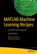
In a more general sense, what does machine learning mean? Machine learning can mean using machines (computers and software) to gain meaning from data. It can also mean giving machines the ability to learn from their environment. Machines have been used to assist humans for thousands of years. Consider a simple lever, which can be fashioned using a rock and a length of wood, or the inclined plane. Both of these machines perform useful work and assist people but neither has the ability to learn. Both are limited by how they are built. Once built, they cannot adapt to changing needs without human interaction. Figure 1.1 shows early machines that do not learn.

../images/420697_2_En_1_Chapter/420697_2_En_1_Fig1_HTML.png — Figure 1.1
Simple machines that do not have the capability to learn.

Both of these machines do useful work and amplify the capabilities of people. The knowledge is inherent in their parameters, which are just the dimensions. The function of the inclined plane is determined by its length and height. The function of the lever is determined by the two lengths and the height. The dimensions are chosen by the designer, essentially building in the designer’s knowledge of the application and physics.

Machine learning involves memory that can be changed while the machine operates. In the case of the two simple machines described above, knowledge is implanted in them by their design. In a sense, they embody the ideas of the builder, and are thus a form of fixed memory. Learning versions of these machines would automatically change the dimensions after evaluating how well the machines were working. As the loads moved or changed the machines would adapt. A modern crane is an example of a machine that adapts to changing loads, albeit at the direction of a human being. The length of the crane can be changed depending on the needs of the operator.

In the context of the software we will be writing in this book, machine learning refers to the process by which an algorithm converts the input data into parameters it can use when interpreting future data. Many of the processes used to mechanize this learning derive from optimization techniques, and in turn are related to the classic field of automatic control. In the remainder of this chapter, we will introduce the nomenclature and taxonomy of machine learning systems.

1.2 Elements of Machine Learning

This section introduces key nomenclature for the field of machine learning.

1.2.1 Data

All learning methods are data driven. Sets of data are used to train the system. These sets may be collected and edited by humans or gathered autonomously by other software tools. Control systems may collect data from sensors as the systems operate and use that data to identify parameters, or train, the system. The data sets may be very large, and it is the explosion of data storage infrastructure and available databases that is largely driving the growth in machine learning software today. It is still true that a machine learning tool is only as good as the data used to create it, and the selection of training data is practically a field unto itself.

Note

When collecting data from training, one must be careful to ensure that the time variation of the system is understood. If the structure of a system changes with time it may be necessary to discard old data before training the system. In automatic control, this is sometimes called a forgetting factor in an estimator.

1.2.2 Models

Models are often used in learning systems. A model provides a mathematical framework for learning. A model is human-derived and based on human observations and experiences. For example, a model of a car, seen from above, might show that it is of rectangular shape with dimensions that fit within a standard parking spot. Models are usually thought of as human-derived and providing a framework for machine learning. However, some forms of machine learning develop their own models without a human-derived structure.

1.2.3 Training

A system, which maps an input to an output, needs training to do this in a useful way. Just as people need to be trained to perform tasks, machine learning systems need to be trained. Training is accomplished by giving the system and input and the corresponding output and modifying the structure (models or data) in the learning machine so that mapping is learned. In some ways, this is like curve fitting or regression. If we have enough training pairs, then the system should be able to produce correct outputs when new inputs are introduced. For example, if we give a face recognition system thousands of cat images and tell it that those are cats we hope that when it is given new cat images it will also recognize them as cats. Problems can arise when you don’t give it enough training sets or the training data are not sufficiently diverse, for instance, identifying a long-haired cat or hairless cat when the training data only consist of shorthaired cats. Diversity of training data is required for a functioning neural net.

1.2.3.1 Supervised Learning

Supervised learning means that specific training sets of data are applied to the system. The learning is supervised in that the “training sets” are human-derived. It does not necessarily mean that humans are actively validating the results. The process of classifying the system’s outputs for a given set of inputs is called “labeling,” that is, you explicitly say which results are correct or which outputs are expected for each set of inputs.

The process of generating training sets can be time consuming. Great care must be taken to ensure that the training sets will provide sufficient training so that when real-world data are collected, the system will produce the correct results. They must cover the full range of expected inputs and desired outputs. The training is followed by test sets to validate the results. If the results aren’t good then the test sets are cycled into the training sets and the process repeated.

A human example would be a ballet dancer trained exclusively in classical ballet technique. If she were then asked to dance a modern dance, the results might not be as good as required because the dancer did not have the appropriate training sets; her training sets were not sufficiently diverse.

1.2.3.2 Unsupervised Learning

Unsupervised learning does not utilize training sets. It is often used to discover patterns in data for which there is no “right” answer. For example, if you used unsupervised learning to train a face identification system the system might cluster the data in sets, some of which might be faces. Clustering algorithms are generally examples of unsupervised learning. The advantage of unsupervised learning is that you can learn things about the data that you might not know in advance. It is a way of finding hidden structures in data.

1.2.3.3 Semi-Supervised Learning

With this approach, some of the data are in the form of labeled training sets and other data are not [11]. In fact, typically only a small amount of the input data is labeled while most are not, as the labeling may be an intensive process requiring a skilled human. The small set of labeled data is leveraged to interpret the unlabeled data.

1.2.3.4 Online Learning

The system is continually updated with new data [11]. This is called “online” because many of the learning systems use data collected online. It could also be called recursive learning. It can be beneficial to periodically “batch” process data used up to a given time and then return to the online learning mode. The spam filtering systems from the introduction utilize online learning.

1.3 The Learning Machine

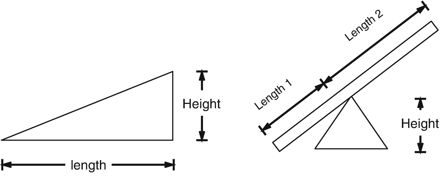
Figure 1.2 shows the concept of a learning machine. The machine absorbs information from the environment and adapts. The inputs may be separated into those that produce an immediate response and those that lead to learning. In some cases they are completely separate. For example, in an aircraft a measurement of altitude is not usually used directly for control. Instead, it is used to help select parameters for the actual control laws. The data required for learning and regular operation may be the same, but in some cases separate measurements or data are needed for learning to take place. Measurements do not necessarily mean data collected by a sensor such as radar or a camera. It could be data collected by polls, stock market prices, data in accounting ledgers or any other means. The machine learning is then the process by which the measurements are transformed into parameters for future operation.

Note that the machine produces output in the form of actions. A copy of the actions may be passed to the learning system so that it can separate the effects of the machine actions from those of the environment. This is akin to a feedforward control system, which can result in improved performance.

A few examples will clarify the diagram. We will discuss a medical example, a security system, and spacecraft maneuvering.

A doctor may want to diagnose diseases more quickly. She would collect data on tests on patients and then collate the results. Patient data may include age, height, weight, historical data such as blood pressure readings and medications prescribed, and exhibited symptoms. The machine learning algorithm would detect patterns so that when new tests were performed on a patient, the machine learning algorithm would be able to suggest diagnoses, or additional tests to narrow down the possibilities. As the machine-learning algorithm were used it would, hopefully, get better with each success or failure. Of course, the definition of success or failure is fuzzy. In this case, the environment would be the patients themselves. The machine would use the data to generate actions, which would be new diagnoses. This system could be built in two ways. In the supervised learning process, test data and known correct diagnoses are used to train the machine. In an unsupervised learning process, the data would be used to generate patterns that may not have been known before and these could lead to diagnosing conditions that would normally not be associated with those symptoms.

../images/420697_2_En_1_Chapter/420697_2_En_1_Fig2_HTML.png — Figure 1.2
A learning machine that senses the environment and stores data in memory.

A security system may be put into place to identify faces. The measurements are camera images of people. The system would be trained with a wide range of face images taken from multiple angles. The system would then be tested with these known persons and its success rate validated. Those that are in the database memory should be readily identified and those that are not should be flagged as unknown. If the success rate were not acceptable, more training might be needed or the algorithm itself might need to be tuned. This type of face recognition is now common, used in Mac OS X’s “Faces” feature in Photos, face identification on the new iPhone X, and Facebook when “tagging” friends in photos.

For precision maneuvering of a spacecraft, the inertia of the spacecraft needs to be known. If the spacecraft has an inertial measurement unit that can measure angular rates, the inertia matrix can be identified. This is where machine learning is tricky. The torque applied to the spacecraft, whether by thrusters or momentum exchange devices, is only known to a certain degree of accuracy. Thus, the system identification must sort out, if it can, the torque scaling factor from the inertia. The inertia can only be identified if torques are applied. This leads to the issue of stimulation. A learning system cannot learn if the system to be studied does not have known inputs and those inputs must be sufficiently diverse to stimulate the system so that the learning can be accomplished. Training a face recognition system with one picture will not work.

1.4 Taxonomy of Machine Learning

In this book, we take a bigger view of machine learning than is typical. Machine learning as described above is the collecting of data, finding patterns, and doing useful things based on those patterns. We expand machine learning to include adaptive and learning control. These fields started off independently, but are now adapting technology and methods from machine learning. Figure 1.3 shows how we organize the technology of machine learning into a consistent taxonomy . You will notice that we created a title that encompasses three branches of learning; we call the whole subject area “Autonomous Learning.” That means, learning without human intervention during the learning process. This book is not solely about “traditional” machine learning. There are other, more specialized books that focus on any one of the machine-learning topics. Optimization is part of the taxonomy because the results of optimization can be new discoveries, such as a new type of spacecraft or aircraft trajectory. Optimization is also often a part of learning systems.

../images/420697_2_En_1_Chapter/420697_2_En_1_Fig3_HTML.png — Figure 1.3
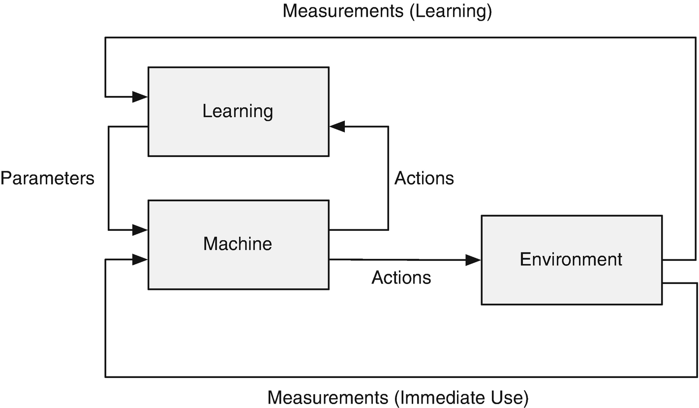
Taxonomy of machine learning.

There are three categories under Autonomous Learning. The first is Control. Feedback control is used to compensate for uncertainty in a system or to make a system behave differently than it would normally behave. If there were no uncertainty you wouldn’t need feedback. For example, if you are a quarterback throwing a football at a running player, assume for a moment and you know everything about the upcoming play. You know exactly where the player should be at a given time, so you can close your eyes, count, and just throw the ball to that spot. Assuming that the player has good hands, you would have a 100% reception rate! More realistically, you watch the player, estimate the player’s speed and throw the ball. You are applying feedback to the problem. As stated, this is not a learning system. However, if now you practice the same play repeatedly, look at your success rate and modify the mechanics and timing of your throw using that information, you would have an adaptive control system, the box second from the top of the control list. Learning in control takes place in adaptive control systems and also in the general area of system identification.

System identification is learning about a system. By system we mean the data that represent the system and the relationships between elements of those data. For example, a particle moving in a straight line is a system defined by its mass, the force on that mass, its velocity and position. The position is related to the velocity times time and the velocity is related determined by the acceleration, which is the force divided by the mass.

Optimal control may not involve any learning. For example, what is known as full state feedback produces an optimal control signal, but does not involve learning. In full state feedback, the combination of model and data tells us everything we need to know about the system. However, in more complex systems we can’t measure all the states and don’t know the parameters perfectly so some form of learning is needed to produce “optimal” or the best possible results.

The second category is what many people consider true Machine Learning. This is making use of data to produce behavior that solves problems. Much of its background comes from statistics and optimization. The learning process may be done once in a batch process or continually in a recursive process. For example, in a stock-buying package, a developer may have processed stock data for several years, say prior to 2008, and used that to decide which stocks to buy. That software may not have worked well during the financial crash. A recursive program would continuously incorporate new data. Pattern recognition and data mining fall into this category. Pattern recognition is looking for patterns in images. For example, the early AI Blocks World software could identify a block in its field of view. It could find one block in a pile of blocks. Data mining is taking large amounts of data and looking for patterns, for example, taking stock market data and identifying companies that have strong growth potential. Classification techniques and fuzzy logic are also in this category.

The third category of autonomous learning is Artificial Intelligence . Machine learning traces some of its origins to artificial intelligence. Artificial Intelligence is the area of study whose goal is to make machines reason. Although many would say the goal is to “think like people,” this is not necessarily the case. There may be ways of reasoning that are not similar to human reasoning, but are just as valid. In the classic Turing test, Turing proposes that the computer only needs to imitate a human in its output to be a “thinking machine,” regardless of how those outputs are generated. In any case, intelligence generally involves learning, so learning is inherent in many Artificial Intelligence technologies such as inductive learning and expert systems. Our diagram includes the two techniques of inductive learning and expert systems.

The recipe chapters of this book are grouped according to this taxonomy. The first chapters cover state estimation using the Kalman Filter and adaptive control. Fuzzy logic is then introduced, which is a control methodology that uses classification. Additional machine-learning recipes follow with chapters on data classification with binary trees, neural nets including deep learning, and multiple hypothesis testing. We then have a chapter on aircraft control that incorporates neural nets, showing the synergy between the different technologies. Finally, we conclude with a chapter on an artificial intelligence technique, case-based expert systems.

1.5 Control

Feedback control algorithms inherently learn about the environment through measurements used for control. These chapters show how control algorithms can be extended to effectively design themselves using measurements. The measurements may be the same as used for control, but the adaptation, or learning, happens more slowly than the control response time. An important aspect of control design is stability. A stable controller will produce bounded outputs for bounded inputs. It will also produce smooth, predictable behavior of the system that is controlled. An unstable controller will typically experience growing oscillations in the quantities (such as speed or position) that is controlled. In these chapters, we explore both the performance of learning control and the stability of such controllers. We often break control into two parts, control and estimation. The latter may be done independent of feedback control.

1.5.1 Kalman Filters

Chapter 4 shows how Kalman filters allow you to learn about dynamical systems for which we already have a model. This chapter provides an example of a variable gain Kalman Filter for a spring system, that is, a system with a mass connected to its base via a spring and a damper. This is a linear system. We write the system in discrete time. This provides an introduction to Kalman Filtering. We show how Kalman Filters can be derived from Bayesian Statistics. This ties it into many machine-learning algorithms. Originally, the Kalman Filter, developed by R. E. Kalman, C. Bucy, and R. Battin, was not derived in this fashion.

The second recipe adds a nonlinear measurement. A linear measurement is a measurement proportional to the state (in this case position) it measures. Our nonlinear measurement will be the angle of a tracking device that points at the mass from a distance from the line of movement. One way is to use an Unscented Kalman Filter (UKF) for state estimation. The UKF lets us use a nonlinear measurement model easily.

The last part of the chapter describes the Unscented Kalman Filter configured for parameter estimation. This system learns the model, albeit one that has an existing mathematical model. As such, it is an example of model-based learning. In this example, the filter estimates the oscillation frequency of the spring-mass system. It will demonstrate how the system needs to be stimulated to identify the parameters.

1.5.2 Adaptive Control

Adaptive control is a branch of control systems in which the gains of the control system change based on measurements of the system. A gain is a number that multiplies a measurement from a sensor to produce a control action such as driving a motor or other actuator. In a nonlearning control system, the gains are computed prior to operation and remain fixed. This works very well most of the time since we can usually pick gains so that the control system is tolerant of parameter changes in the system. Our gain “margins” tell us how tolerant we are to uncertainties in the system. If we are tolerant to big changes in parameters, we say that our system is robust.

Adaptive control systems change the gain based on measurements during operation. This can help a control system perform even better. The better we know a system’s model, the tighter we can control the system. This is much like driving a new car. At first, you have to be cautious driving a new car, because you don’t know how sensitive the steering is to turning the wheel or how fast it accelerates when you depress the gas pedal. As you learn about the car you can maneuver it with more confidence. If you didn’t learn about the car you would need to drive every car in the same fashion.

Chapter 5 starts with a simple example of adding damping to a spring using a control system. Our goal is to get a specific damping time constant. For this, we need to know the spring constant. Our learning system uses a Fast Fourier Transform to measure the spring constant. We’ll compare it with a system that does know the spring constant. This is an example of tuning a control system. The second example is model reference adaptive control of a first-order system. This system automatically adapts so that the system behaves like the desired model. This is a very powerful method and applicable to many situations. An additional example will be ship steering control. Ships use adaptive control because it is more efficient than conventional control. This example demonstrates how the control system adapts and how it performs better than its non-adaptive equivalent. This is an example of gain scheduling. We then give a spacecraft example.

The last example is longitudinal control of an aircraft, extensive enough that it is given its own chapter. We can control pitch angle using the elevators. We have five nonlinear equations for the pitch rotational dynamics, velocity in the x direction, velocity in the z direction, and change in altitude. The system adapts to changes in velocity and altitude. Both change the drag and lift forces and the moments on the aircraft and also change the response to the elevators. We use a neural net as the learning element of our control system. This is a practical problem applicable to all types of aircraft ranging from drones to high-performance commercial aircraft.

1.6 Autonomous Learning Methods

This section introduces you to popular machine-learning techniques. Some will be used in the examples in this book. Others are available in MATLAB products and open-source products.

1.6.1 Regression

Regression is a way of fitting data to a model. A model can be a curve in multiple dimensions. The regression process fits the data to the curve producing a model that can be used to predict future data. Some methods, such as linear regression or least squares, are parametric in that the number of parameters to be fit is known. An example of linear regression is shown in the listing below and Figure 1.4. This model was created by starting with the line y = x and adding noise to y. The line was recreated using a least squares fit via MATLAB’s pinv Pseudo-inverse function.

The first part of the script generates the data.

Listing 1.1 Linear Regression to Data Generation

x = linspace (0,1,500)’;

n = length (x);

% Model a polynomial, y = ax2 + mx + b

a = 1.0; % quadratic - make nonzero for larger errors

m = 1.0; % slope

b = 1.0; % intercept

sigma = 0.1; % standard deviation of the noise

y0 = a*x.^2 + m*x + b;

y = y0 + sigma* randn (n,1);

The actual regression code is just three lines.

Listing 1.2 Linear Regression

a = [x ones(n,1)];

c = pinv(a)*y;

yR = c(1)*x + c(2); % the fitted line

The last part plots the results using standard MATLAB plotting functions. We use grid on rather than grid. The latter toggles the grid mode and is usually ok, but sometimes MATLAB gets confused. grid on is more reliable.

Listing 1.3 Linear Regression to Plots

h = figure ;

h.Name = ’Linear␣Regression’;

plot(x,y); hold on;

plot(x,yR, ’linewidth’,2);

grid on

xlabel( ’x’);

ylabel( ’y’);

title( ’Linear␣Regression’);

legend( ’Data’, ’Fit’)

figure( ’Name’, ’Regression␣Error’)

plot(x,yR-y0);

grid on

xlabel( ’x’);

ylabel( ’\Delta␣y’);

title( ’Error␣between␣Model␣and␣Regression’)

This code uses pinv. We can solve the problem

$\displaystyle \begin{aligned} Ax =b \end{aligned}$

(1.1)

by taking the inverse of A if the length of x and b are the same.

$\displaystyle \begin{aligned} x = A^{-1}b \end{aligned}$

(1.2)

This works because A is a square matrix, but only works if A is not singular, that is, it has a valid inverse. If the length of x and b are the same, we can still find an approximation to x where x = pinv(A)b. For example, in the first case A is 2-by-2. In the second case, it is 3-by-2, meaning there are three elements of x and two of b.

>> inv ( rand (2,2))

ans =

1.4518 -0.2018

-1.4398 1.2950

>> pinv ( rand (2,3))

ans =

1.5520 -1.3459

-0.6390 1.0277

0.2053 0.5899

The system learns the parameters, slope, and y intercept, from the data. The more data, the better the fit. As it happens, our model:

$\displaystyle \begin{aligned} y = mx + b \end{aligned}$

(1.3)

is correct. However, if it were wrong, the fit would be poor. This is an issue with model-based learning. The quality of the results is highly dependent on the model. If you are sure of your model then it should be used. If not, other methods, such as unsupervised learning, may produce better results. For example, if we add the quadratic term x ², we get the fit in Figure 1.5. Notice how the fit is not as good as we might like.

In these examples, we start with a pattern that we assume fits the data. This is our model. We fit the data to the model. In the first case, we assume that our system is linear; in the second quadratic. If our model is good, the data will fit well. If we choose the wrong model, then the fit will be poor. If that is the case, we will need to try a different model. For example, our system could be

$\displaystyle \begin{aligned} y = \cos{}(x) \end{aligned}$

(1.4)

with the span of x over several cycles. Neither a linear nor a quadratic fit would be good in this case. Limitations in this approach have led to other techniques, including neural networks.

../images/420697_2_En_1_Chapter/420697_2_En_1_Fig4_HTML.png — Figure 1.4
Learning with linear regression.

../images/420697_2_En_1_Chapter/420697_2_En_1_Fig5_HTML.png — Figure 1.5
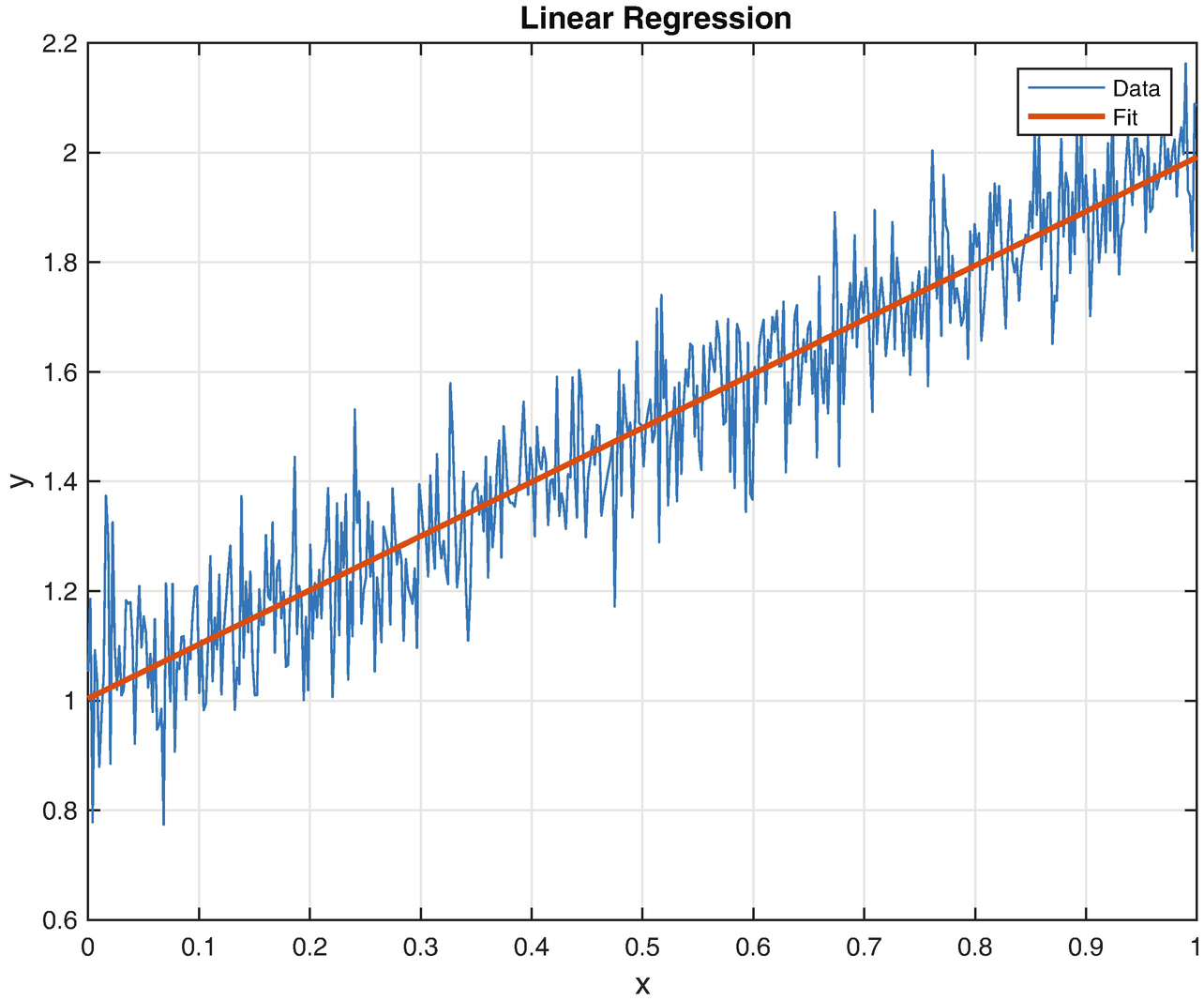
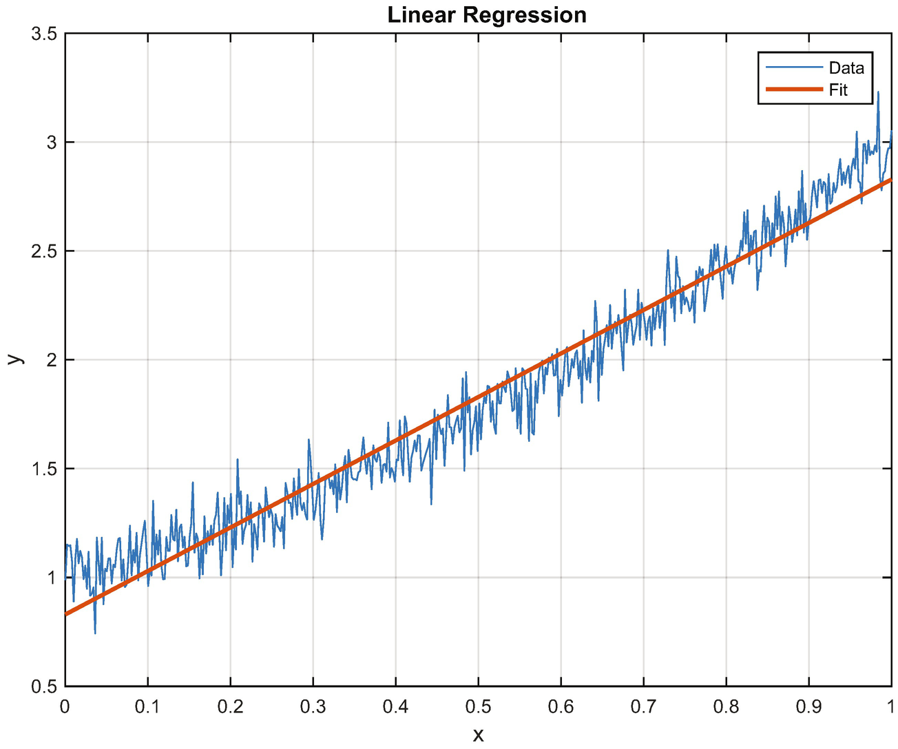
Learning with linear regression for a quadratic.

1.6.2 Decision Trees

A decision tree is a tree-like graph used to make decisions. It has three kinds of nodes:

1.
Decision nodes
2.
Chance nodes
3.
End nodes

You follow the path from the beginning to the end node. Decision trees are easy to understand and interpret. The decision process is entirely transparent, although very large decision trees may be hard to follow visually. The difficulty is finding an optimal decision tree for a set of training data.

Two types of decision trees are classification trees that produce categorical outputs and regression trees that produce numeric outputs. An example of a classification tree is shown in Figure 1.6. This helps an employee decide where to go for lunch. This tree only has decision nodes.

../images/420697_2_En_1_Chapter/420697_2_En_1_Fig6_HTML.png — Figure 1.6
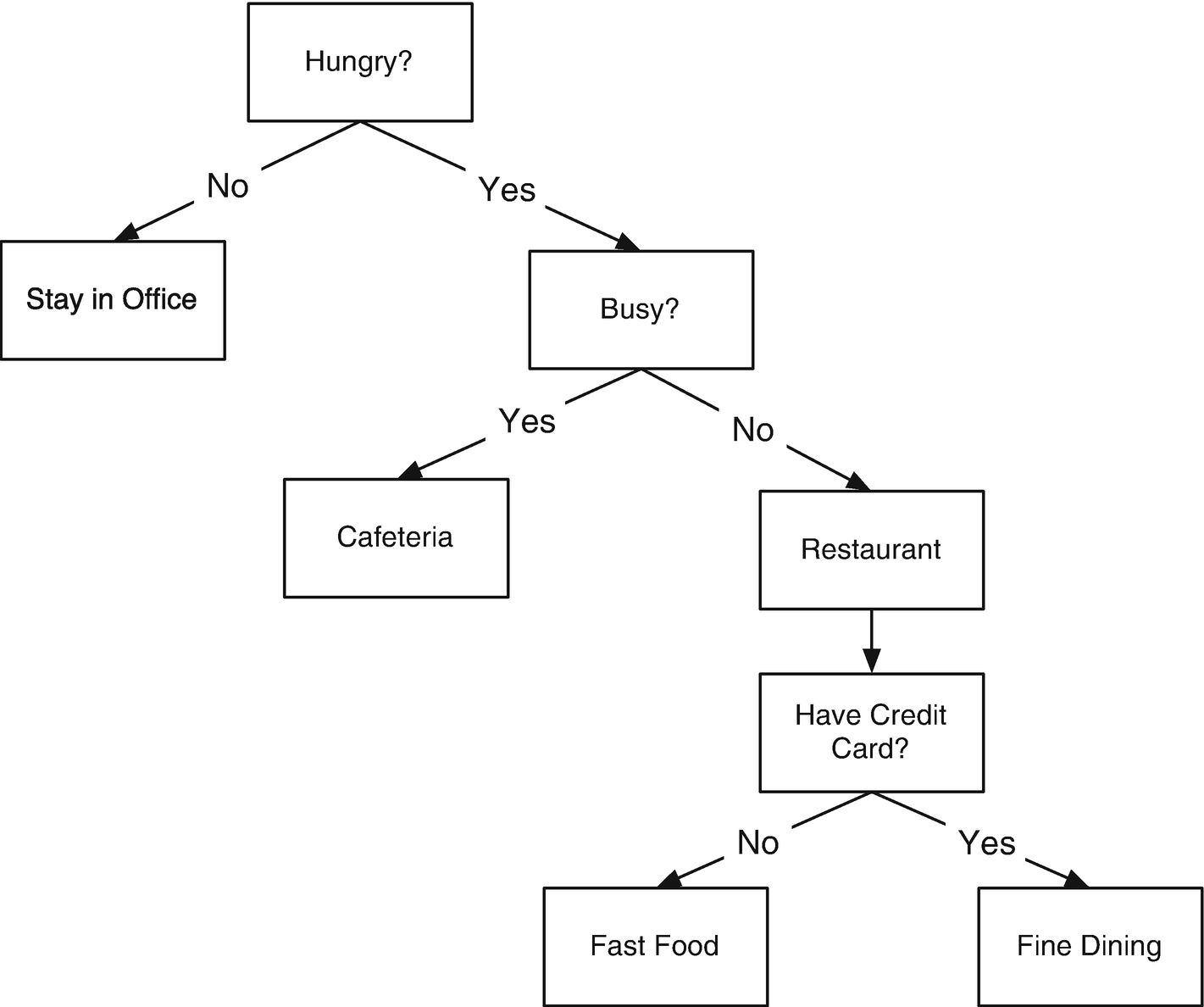
A classification tree.

This may be used by management to predict where they could find an employee at lunch time. The decisions are Hungry, Busy, and Have a Credit Card. From that, the tree could be synthesized. However, if there were other factors in the decision of employees, for example, is it someone’s birthday, this would result in the employee going to a restaurant, then the tree would not be accurate.

Chapter 7 uses a decision tree to classify data. Classifying data is one of the most widely used areas of machine learning. In this example, we assume that two data points are sufficient to classify a sample and determine to which group it belongs. We have a training set of known data points with membership in one of three groups. We then use a decision tree to classify the data. We’ll introduce a graphical display to make understanding the process easier.

With any learning algorithm it is important to know why the algorithm made its decision. Graphics can help you explore large data sets when columns of numbers aren’t terribly helpful.

1.6.3 Neural Networks

A neural net is a network designed to emulate the neurons in a human brain. Each “neuron” has a mathematical model for determining its output from its input; for example, if the output is a step function with a value of 0 or 1, the neuron can be said to be “firing” if the input stimulus results in a 1 output. Networks are then formed with multiple layers of interconnected neurons. Neural networks are a form of pattern recognition. The network must be trained using sample data, but no a priori model is required. However, usually, the structure of the neural network is specified by giving the number of layers, neurons per layer, and activation functions for each neuron. Networks can be trained to estimate the output of nonlinear processes and the network then becomes the model.

Figure 1.7 displays a simple neural network that flows from left to right, with two input nodes and one output node. There is one “hidden” layer of neurons in the middle. Each node has a set of numeric weights that is tuned during training. This network has two inputs and one output, possibly indicative of a network that solves a categorization problem. Training such a network is called deep learning.

A “deep” neural network is a neural network with multiple intermediate layers between the input and output.

This book presents neural nets in several chapters. Chapter 8 provides an introduction to the fundamentals of neural networks focusing on the neuron and how it can be trained. Chapter 9 provides an introduction to neural networks using a multi-layer feed-forward (MLFF) neural network to classify digits. In this type of network, each neuron depends only on the inputs it receives from the previous layer. The example uses a neural network to classify digits. We will start with a set of six digits and create a training set by adding noise to the digit images. We then see how well our learning network performs at identifying a single digit, and then add more nodes and outputs to identify multiple digits with one network. Classifying digits is one of the oldest uses of machine learning. The U.S. Post Office introduced zip code reading years before machine learning started hitting the front pages of all the newspapers! Earlier digit readers required block letters written in well-defined spots on a form. Reading digits off any envelope is an example of learning in an unstructured environment.

../images/420697_2_En_1_Chapter/420697_2_En_1_Fig7_HTML.png — Figure 1.7
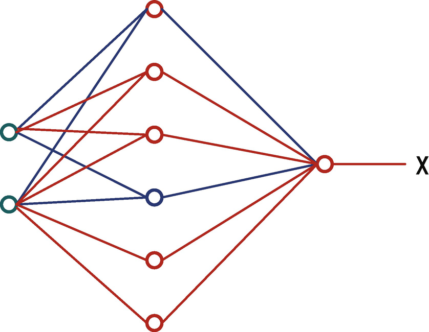
A neural net with one intermediate layer between the inputs on the left and the output on the right. The intermediate layer is also known as a hidden layer.

Chapter 10 presents deep learning with distinctive layers. Several different types of elements are in the deep learning chain. This is applied to face recognition. Face recognition is available in almost every photo application. Many social media sites, such as Facebook and Google Plus, also use face recognition. Cameras have built-in face recognition, though not identification, to help with focusing when taking portraits. Our goal is to get the algorithm to match faces, not classify them. Data classification is covered in Chapter 8.

Chapter 11 introduces a neural network as part of an adaptive control system. This ties together learning, via neural networks, and control.

1.6.4 Support Vector Machines

Support vector machines (SVMs) are supervised learning models with associated learning algorithms that analyze data used for classification and regression analysis. An SVM training algorithm builds a model that assigns examples into categories. The goal of SVMs is to produce a model, based on the training data, that predicts the target values.

In SVMs, nonlinear mapping of input data in a higher dimensional feature space is done with kernel functions. In this feature space, a separation hyperplane is generated that is the solution to the classification problem. The kernel functions can be polynomials, sigmoidal functions, and radial basis functions. Only a subset of the training data is needed, these are known as the support vectors [8]. The training is done by solving a quadratic program, which can be done with many numerical software.

1.7 Artificial Intelligence

1.7.1 What is Artificial Intelligence?

A test of artificial intelligence is the Turing test. The idea is that if you have a conversation with a machine and you can’t tell it is a machine, then it should be considered intelligent. By this definition, many robo-calling systems might be considered intelligent. Another example, chess programs, can beat all but the best players, but a chess program can’t do anything but play chess. Is a chess program intelligent? What we have now is machines that can do things pretty well in a particular context.

1.7.2 Intelligent Cars

Our “artificial intelligence” example is really a blending of Bayesian estimation and controls. It still reflects a machine doing what we would consider as intelligent behavior. This, of course, gets back to the question of defining intelligence.

Autonomous driving is an area of great interest to automobile manufacturers and to the general public. Autonomous cars are driving the streets today, but are not yet ready for general use by the public. There are many technologies involved in autonomous driving. These include:

1.
Machine vision – turning camera data into information useful for the autonomous control system
2.
Sensing – using many technologies including vision, radar, and sound to sense the environment around the car
3.
Control – using algorithms to make the car go where it is supposed to go as determined by the navigation system
4.
Machine learning – using massive data from test cars to create databases of responses to situations
5.
GPS navigation – blending GPS measurements with sensing and vision to figure out where to go
6.
Communications/ad hoc networks – talking with other cars to help determine where they are and what they are doing

All of the areas overlap. Communications and ad hoc networks are used with GPS navigation to determine both absolute location (what street and address corresponds to your location) and relative navigation (where you are with respect to other cars). In this context, the Turing test would be if you couldn’t tell if a car was driven by a person or the computer. Now, since many drivers are bad, one could argue that a computer that drove really well would fail the Turing test! This gets back to the question of what intelligence is.

This example explores the problem of a car being passed by multiple cars and needing to compute tracks for each one. We are really addressing just the control and collision avoidance problem. A single sensor version of Track Oriented Multiple Hypothesis Testing is demonstrated for a single car on a two-lane road. The example includes MATLAB graphics that make it easier to understand the thinking of the algorithm. The demo assumes that the optical or radar pre-processing has been done and that each target is measured by a single “blip” in two dimensions. An automobile simulation is included. It involves cars passing the car that is doing the tracking. The passing cars use a passing control system that is in itself a form of machine intelligence.

Our autonomous driving recipes use an Unscented Kalman Filter for the estimation of the state. This is the underlying algorithm that propagates the state (that is, advances the state in time in a simulation) and adds measurements to the state. A Kalman Filter, or other estimator, is the core of many target-tracking systems.

The recipes will also introduce graphics aids to help you understand the tracking decision process. When you implement a learning system you want to make sure it is working the way you think it should, or understand why it is working the way it does.

1.7.3 Expert Systems

A system that uses a knowledge base to reason and present the user with a result and an explanation of how it arrived at that result. Expert systems are also known as knowledge-based systems. The process of building an expert system is called knowledge engineering. This involves a knowledge engineer, someone who knows how to build the expert system, interviewing experts for the knowledge needed to build the system. Some systems can induce rules from data, speeding up the data acquisition process.

An advantage of expert systems, over human experts, is that knowledge from multiple experts can be incorporated into the database. Another advantage is that the system can explain the process in detail so that the user knows exactly how the result was generated. Even an expert in a domain can forget to check certain things. An expert system will always methodically check its full database. It is also not affected by fatigue or emotions.

Knowledge acquisition is a major bottleneck in building expert systems. Another issue is that the system cannot extrapolate beyond what is programmed into the database. Care must be taken with using an expert system because it will generate definitive answers for problems where there is uncertainty. The explanation facility is important, because someone with domain knowledge can judge the results from the explanation. In cases where uncertainty needs to be considered, a probabilistic expert system is recommended. A Bayesian network can be used as an expert system. A Bayesian network is also known as a belief network. It is a probabilistic graphical model that represents a set of random variables and their dependencies. In the simplest cases, a Bayesian network can be constructed by an expert. In more complex cases, it needs to be generated from data from machine learning. Chapter 12 delves into expert systems.

In Chapter 14, we explore a simple case-based reasoning system. An alternative would be a rule-based system.

1.8 Summary

All of the technologies in this chapter are in current use today. Any one of them can form the basis for a useful product. Many systems, such as autonomous cars, use several. We hope that our broad view of the field of machine learning and our unique taxonomy, which shows the relationships of machine learning and artificial intelligence to the classical fields of control and optimization, are useful to you. In the remainder of the book we will show you how to build software that implements these technologies. This can form the basis of your own more robust production software, or help you to use the many fine commercial products more effectively. Table 1.1 lists the scripts included in the companion code.

Table 1.1

Chapter Code Listing

File	Description
LinearRegression	A script that demonstrates linear regression and curve fitting.

Previous Chapter

Front Matter

Next Chapter

2. Representation of Data for Machine Learning in MATLAB