© Michael Paluszek and Stephanie Thomas  2019
Michael Paluszek and Stephanie ThomasMATLAB Machine Learning Recipeshttps://doi.org/10.1007/978-1-4842-3916-2_11

11. Neural Aircraft Control

Michael Paluszek1  and Stephanie Thomas1
(1)
Plainsboro, NJ, USA
 

Longitudinal control is the control of an aircraft that needs to work at the altitude and speed changes. In this chapter, we will implement a neural net to produce the critical parameters for a nonlinear aircraft control system. This is an example of online learning and applies techniques from multiple previous chapters.

../images/420697_2_En_11_Chapter/420697_2_En_11_Figa_HTML.gif

The longitudinal dynamics of an aircraft are also known as the pitch dynamics. The dynamics are entirely in the plane of symmetry of the aircraft. The plane of symmetry is defined as a plane that cuts the aircraft in half vertically. Most airplanes are symmetric about this plane. These dynamics include the forward and vertical motion of the aircraft and the pitching of the aircraft about the axis perpendicular to the plane of symmetry. Figure 11.1 shows an aircraft in flight. α is the angle-of-attack, the angle between the wing and the velocity vector. We assume that the wind direction is opposite that of the velocity vector, that is, the aircraft produces all of its wind. Drag is along the wind direction and lift is perpendicular to drag. The pitch moment is around the center of mass. The model we will derive uses a small set of parameters, yet reproduces the longitudinal dynamics reasonably well. It is also easy for you to modify the model to simulate any aircraft of interest.
../images/420697_2_En_11_Chapter/420697_2_En_11_Fig1_HTML.png
Figure 11.1

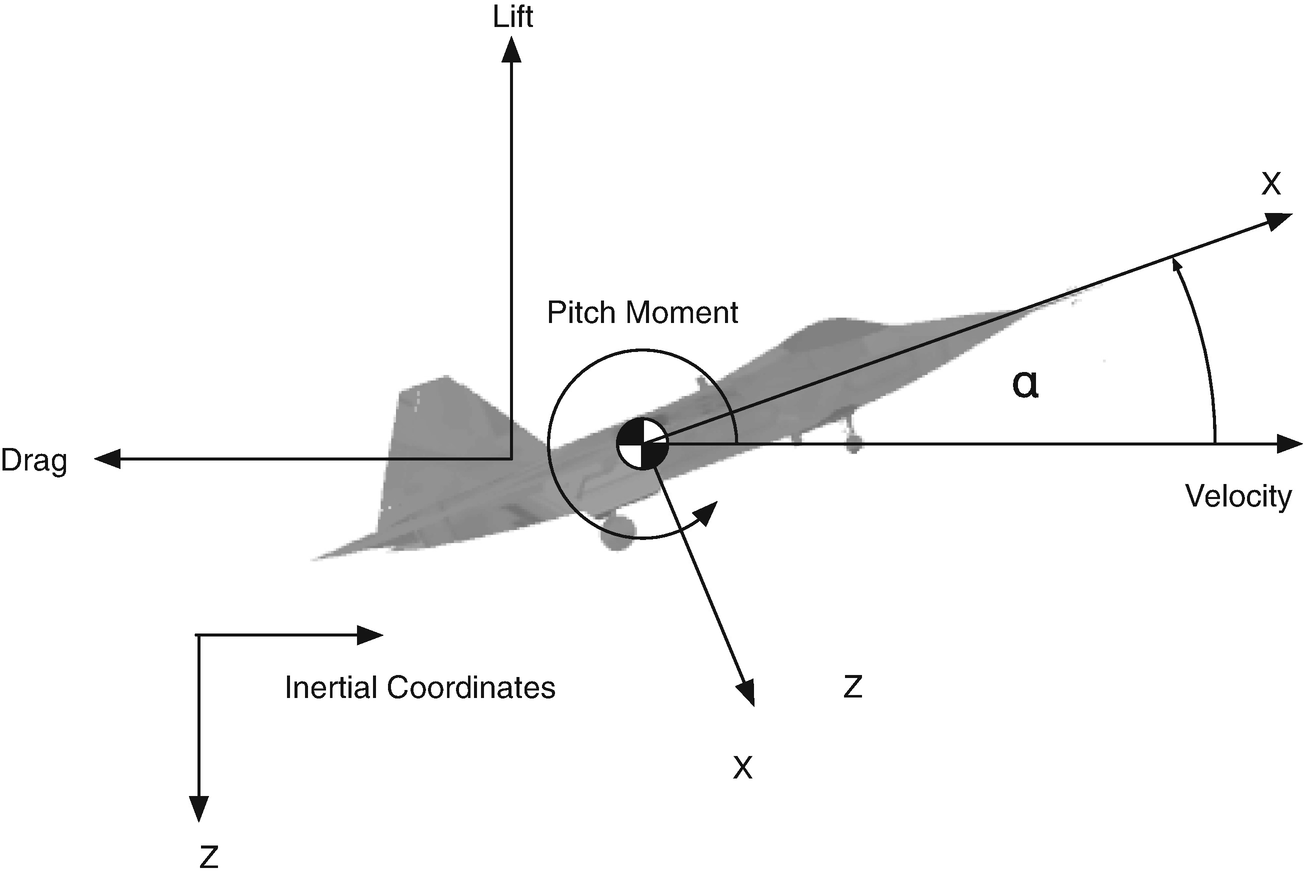
Diagram of an aircraft in flight showing all the important quantities for longitudinal dynamics simulation.

11.1 Longitudinal Motion

The next few recipes will involve the longitudinal control of an aircraft with a neural net to provide learning. We will:
  1. 1.

    Model the aircraft dynamics

     
  2. 2.

    Find an equilibrium solution about which we will control the aircraft

     
  3. 3.

    Learn how to write a sigma-pi neural net

     
  4. 4.

    Implement the PID control

     
  5. 5.

    Implement the neural net

     
  6. 6.

    Simulate the system


In this recipe, we will model the longitudinal dynamics of an aircraft for use in learning control. We will derive a simple longitudinal dynamics model with a “small” number of parameters. Our control will use nonlinear dynamics inversion with a proportional integral differential (PID) controller to control the pitch dynamics [16, 17]. Learning will be done using a sigma-pi neural network.

We will use the learning approach developed at NASA Dryden Research Center [30]. The baseline controller is a dynamic inversion type controller with a PID control law. A neural net [15] provides learning while the aircraft is operating. The neural network is a sigma-pi type network meaning that the network sums the products of the inputs with their associated weights. The weights of the neural network are determined by a training algorithm that uses:
  1. 1.

    Commanded aircraft rates from the reference model

     
  2. 2.

    PID errors

     
  3. 3.

    Adaptive control rates fed back from the neural network


11.1.1 Problem

We want to model the longitudinal dynamics of an aircraft.

11.1.2 Solution

The solution is to write the right-hand side function for the aircraft longitudinal dynamics differential equations.

11.1.3 How It Works

We summarized the symbols for the dynamical model in Table 11.1

Our aerodynamic model is very simple. The lift and drag are:
$$\displaystyle \begin{aligned} \begin{array}{rcl} L = pSC_L \end{array} \end{aligned} $$
(11.1)
$$\displaystyle \begin{aligned} \begin{array}{rcl} D =pSC_D \end{array} \end{aligned} $$
(11.2)
where S is the wetted area, the area that interacts with the airflow and is the area that is counted in computing the aerodynamic forces, and p is the dynamic pressure, the pressure on the aircraft caused by its velocity:
$$\displaystyle \begin{aligned} p = \frac{1}{2}\rho v^2 \end{aligned} $$
(11.3)
where ρ is the atmospheric density and v is the magnitude of the velocity. Atmospheric density is a function of altitude. For low-speed flight this is mostly the wings. Most books use q for dynamic pressure. We use q for pitch angular rate (also a convention), so we use p for pressure here to avoid confusion.
The lift coefficient, CL is:
$$\displaystyle \begin{aligned} C_L = C_{L_\alpha}\alpha \end{aligned} $$
(11.4)
and the drag coefficient, CD is:
$$\displaystyle \begin{aligned} C_D = C_{D_0} + kC_L^2 \end{aligned} $$
(11.5)
The drag equation is called the drag polar. Increasing the angle of attack increases the aircraft lift, but also increases the aircraft drag. The coefficient k is:
$$\displaystyle \begin{aligned} k = \frac{1}{\pi \epsilon_0 AR} \end{aligned} $$
(11.6)
Table 11.1

Aircraft Dynamics Symbols

Symbol

Description

Units

g

Acceleration of gravity at sea-level

9.806 m/s2

h

Altitude

m

k

Coefficient of lift induced drag


m

Mass

kg

p

Dynamic pressure

N/m2

q

Pitch angular rate

rad/s

u

x-velocity

m/s

w

z-velocity

m/s

C L

Lift coefficient


C D

Drag coefficient


D

Drag

N

I y

Pitch moment of inertia

kg-m2

L

Lift

N

M

Pitch moment (torque)

Nm

M e

Pitch moment due to elevator

Nm

r e

Elevator moment arm

m

S

Wetted area of wings (the area that contributes to lift and drag)

m2

S e

Wetted area of elevator

m2

T

Thrust

N

X

X force in the aircraft frame

N

Z

Z force in the aircraft frame

N

α

Angle of attack

rad

γ

Flight path angle

rad

ρ

Air density

kg/m3

θ

Pitch angle

rad

where 𝜖 0 is the Oswald efficiency factor, which is typically between 0.75 and 0.85. AR is the wing aspect ratio. The aspect ratio is the ratio of the span of the wing to its chord. For complex shapes, it is approximately given by the formula:
$$\displaystyle \begin{aligned} AR = \frac{b^2}{S} \end{aligned} $$
(11.7)
where b is the span and S is the wing area. Span is measured from wingtip to wingtip. Gliders have very high aspect ratios and delta-wing aircraft have low aspect ratios.

The aerodynamic coefficients are nondimensional coefficients that when multiplied by the wetted area of the aircraft, and the dynamic pressure, produce the aerodynamic forces.
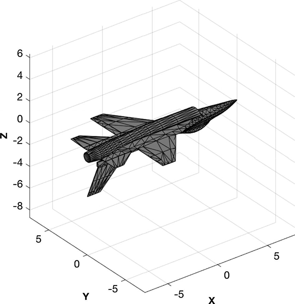
The dynamical equations, the differential equations of motion, are [5]:
$$\displaystyle \begin{aligned} \begin{array}{rcl} m(\dot{u} +qw) &\displaystyle =&\displaystyle X - mg\sin\theta +T\cos\epsilon \end{array} \end{aligned} $$
(11.8)
$$\displaystyle \begin{aligned} \begin{array}{rcl} m(\dot{w}-qu) &\displaystyle =&\displaystyle Z + mg\cos\theta -T\sin\epsilon \end{array} \end{aligned} $$
(11.9)
$$\displaystyle \begin{aligned} \begin{array}{rcl} I_y\dot{q} &\displaystyle =&\displaystyle M \end{array} \end{aligned} $$
(11.10)
$$\displaystyle \begin{aligned} \begin{array}{rcl} \dot{\theta} &\displaystyle =&\displaystyle q \end{array} \end{aligned} $$
(11.11)
m is the mass, u is the x-velocity, w is the z-velocity, q is the pitch angular rate, θ is the pitch angle, T is the engine thrust, 𝜖 is the angle between the thrust vector and the x-axis, Iy is the pitch inertia, X is the x-force, Z is the z-force, and M is the torque about the pitch axis. The coupling between x and z velocities is due to writing the force equations in the rotating frame. The pitch equation is about the center of mass. These are a function of u, w, q, and altitude, h, which is found from:
$$\displaystyle \begin{aligned} \dot{h} = u\sin\theta - w\cos\theta \end{aligned} $$
(11.12)
The angle of attack, α is the angle between the u and w velocities and is:
$$\displaystyle \begin{aligned} \tan\alpha = \frac{w}{u} \end{aligned} $$
(11.13)
The flight path angle γ is the angle between the vector velocity direction and the horizontal. It is related to θ and α by the relationship:
$$\displaystyle \begin{aligned} \gamma = \theta - \alpha \end{aligned} $$
(11.14)
This does not appear in the equations, but it is useful to compute when studying aircraft motion. The forces are:
$$\displaystyle \begin{aligned} \begin{array}{rcl} X &\displaystyle =&\displaystyle L\sin\alpha - D\cos\alpha \end{array} \end{aligned} $$
(11.15)
$$\displaystyle \begin{aligned} \begin{array}{rcl} Z &\displaystyle =&\displaystyle -L\cos\alpha - D\sin\alpha \end{array} \end{aligned} $$
(11.16)
The moment, or torque, is assumed because of the offset of the center-of-pressure and center of mass, which is assumed to be along the x-axis:
$$\displaystyle \begin{aligned} M = (c_p-c)Z \end{aligned} $$
(11.17)
where cp is the location of the center of pressure. The moment due to the elevator is:
$$\displaystyle \begin{aligned} M_e = qr_eS_e\sin{}(\delta) \end{aligned} $$
(11.18)
Se is the wetted area of the elevator and rE is the distance from the center of mass to the elevator. The dynamical model is in RHSAircraft. The atmospheric density model is an exponential model and is included as a subfunction in this function. RHSAircraft returns the default data structure if no inputs are given.
function [xDot, lift, drag, pD] = RHSAircraft( ~, x, d )
ifnargin < 1 )
   xDot = DataStructure;
    return
end
 g     = 9.806;  % Acceleration of gravity (m/s^2)
 u     = x(1);  % Forward velocity
 w     = x(2);  % Up velocity
 q     = x(3);  % Pitch angular rate
 theta = x(4);  % Pitch angle
 h     = x(5);  % Altitude
 rho   = AtmDensity( h );  % Density in kg/m^3
 alpha =  atan (w/u);
 cA    =  cos (alpha);
 sA    =  sin (alpha);
 v     =  sqrt (u^2 + w^2);
 pD    = 0.5*rho*v^2;  % Dynamic pressure
 cL    = d.cLAlpha*alpha;
 cD    = d.cD0 + d.k*cL^2;
 drag  = pD*d.s*cD;
 lift  = pD*d.s*cL;
 x     =  lift*sA - drag*cA;
 z     = -lift*cA - drag*sA;
 m     =  d.c*z + pD*d.sE*d.rE* sin (d.delta);
 sT    =  sin (theta);
 cT    =  cos (theta);
 tEng  = d.thrust*d.throttle;
 cE    =  cos (d.epsilon);
 sE    =  sin (d.epsilon);
 uDot  = (x + tEng*cE)/d.mass - q*w - g*sT + d.externalAccel(1);
 wDot  = (z - tEng*sE)/d.mass + q*u + g*cT + d.externalAccel(2);
 qDot  = m/d.inertia                       + d.externalAccel(3);
 hDot  = u*sT - w*cT;
 xDot  = [uDot;wDot;qDot;q;hDot];
We will use a model of the F-16 aircraft for our simulation. The F-16 is a single engine supersonic multi-role combat aircraft used by many countries. The F-16 is shown in Figure 11.2.
../images/420697_2_En_11_Chapter/420697_2_En_11_Fig2_HTML.jpg
Figure 11.2

F-16 model.

The inertia matrix is found by taking this model, distributing the mass amongst all the vertices, and computing the inertia from the formulas
$$\displaystyle \begin{aligned} \begin{array}{rcl} m_k &amp;\displaystyle =&amp;\displaystyle \frac{m}{N} \end{array} \end{aligned} $$
(11.19)
$$\displaystyle \begin{aligned} \begin{array}{rcl} c &amp;\displaystyle =&amp;\displaystyle \sum_k m_k r_k \end{array} \end{aligned} $$
(11.20)
$$\displaystyle \begin{aligned} \begin{array}{rcl} I &amp;\displaystyle =&amp;\displaystyle \sum_k m_k(r_k-c)^2 \end{array} \end{aligned} $$
(11.21)
where N is the number of nodes and rk is the vector from the origin (which is arbitrary) to node k.
 inr =
    1.0e+05 *
     0.3672    0.0002   -0.0604
     0.0002    1.4778    0.0000
    -0.0604    0.0000    1.7295  
The F-16 data are given in Table 11.2.
Table 11.2

F-16 Data

Symbol

Field

Value

Description

Units

$$C_{L_\alpha }$$

cLAlpha

6.28

Lift coefficient


$$C_{D_0}$$

cD0

0.0175

Zero lift drag coefficient


k

k

0.1288

Lift coupling coefficient


𝜖

epsilon

0

Thrust angle from the x-axis

rad

T

thrust

76.3e3

Engine thrust

N

S

s

27.87

Wing area

m2

m

mass

12,000

Aircraft mass

kg

I y

inertia

1.7295e5

z-axis inertia

kg-m2

c − cp

c

1

Offset of center-of-mass from the center-of-pressure

m

S e

sE

3.5

Elevator area

m2

r e

( rE)

4.0

Elevator moment arm

m

There are many limitations to this model. First of all, the thrust is applied immediately with 100% accuracy. The thrust is also not a function of airspeed or altitude. Real engines take some time to achieve the commanded thrust and the thrust levels change with airspeed and altitude. In the model, the elevator also responds instantaneously. Elevators are driven by motors, usually hydraulic, but sometimes pure electric, and they take time to reach a commanded angle. In our model, the aerodynamics are very simple. In reality, lift and drag are complex functions of airspeed and angle of attack and are usually modeled with large tables of coefficients. We also model the pitching moment by a moment arm. Usually, the torque is modeled by a table. No aerodynamic damping is modeled although this appears in most complete aerodynamic models for aircraft. You can easily add these features by creating functions:

 C_L = CL(v,h,alpha,delta)
 C_D = CD(v,h,alpha,delta)
 C_M = CL(v,h,vdot,alpha,delta)  

11.2 Numerically Finding Equilibrium

11.2.1 Problem

We want to determine the equilibrium state for the aircraft. This is the orientation at which all forces and torques balance.

11.2.2 Solution

The solution is to compute the Jacobian for the dynamics. The Jacobian is a matrix of all first-order partial derivatives of a vector valued function, in this case the dynamics of the aircraft.

11.2.3 How It Works

We want to start every simulation from an equilibrium state. This is done using the function EquilibriumState. It uses fminsearch to minimize:
$$\displaystyle \begin{aligned} \dot{u}^2 + \dot{w}^2 \end{aligned} $$
(11.22)
given the flight speed, altitude, and flight path angle. It then computes the elevator angle needed to zero the pitch angular acceleration. It has a built-in demo for equilibrium level flight at 10 km.
function [x, thrust, delta, cost] = EquilibriumState( gamma, v, h, d )
  %% Code
ifnargin < 1 )
   Demo;
    return
end
  % [Forward velocity, vertical velocity, pitch rate pitch angle and altitude
 x             = [v;0;0;0;h];
 [~,~,drag]    = RHSAircraft( 0, x, d );
 y0            = [0;drag];
 cost(1)       = CostFun( y0, d,  gamma , v, h );
 y             = fminsearch( @CostFun, y0, [], d,  gamma , v, h );
 w             = y(1);
 thrust        = y(2);
 u             =  sqrt (v^2-w^2);
 alpha         =  atan (w/u);
 theta         =  gamma  + alpha;
 cost(2)       = CostFun( y, d,  gamma , v, h );
 x             = [u;w;0;theta;h];
 d.thrust      = thrust;
 d.delta       = 0;
 [xDot,~,~,p]  = RHSAircraft( 0, x, d );  

CostFun is the cost functional given below.

function cost = CostFun ( y, d, gamma, v, h )
  %% EquilibriumState>CostFun
  % Cost function for fminsearch. The cost is the square of the velocity
  % derivatives (the first two terms of xDot from RHSAircraft).
  %
  % See also RHSAircraft.
 w         = y(1);
 d.thrust       = y(2);
 d.delta   = 0;
 u         =  sqrt (v^2-w^2);
 alpha     =  atan (w/u);
 theta     = gamma + alpha;
 x         = [u;w;0;theta;h];
 xDot      = RHSAircraft( 0, x, d );
 cost      = xDot(1:2)’*xDot(1:2);

The vector of values is the first input. Our first guess is that thrust equals drag. The vertical velocity and thrust are solved for by fminsearch. fminsearch searches over thrust and vertical velocity to find an equilibrium state.

The results of the demo are:

 >> EquilibriumState
 Velocity            250.00 m/s
 Altitude          10000.00 m
 Flight path angle     0.00 deg
 Z speed              13.84 m/s
 Thrust            11148.95 N
 Angle of attack       3.17 deg
 Elevator            -11.22 deg
 Initial cost      9.62e+01
 Final cost        1.17e-17  

The initial and final costs show how successful fminsearch was in achieving the objective of minimizing the w and u accelerations.

11.3 Numerical Simulation of the Aircraft

11.3.1 Problem

We want to simulate the aircraft.

11.3.2 Solution

The solution is to create a script that calls the right-hand side of the dynamical equations, RHSAircraft in a loop, and plot the results.

11.3.3 How It Works

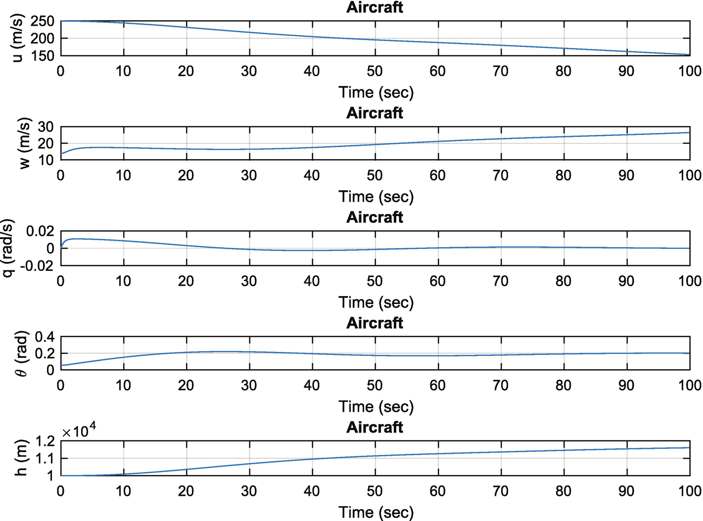
The simulation script is shown below. It computes the equilibrium state, then simulates the dynamics in a loop by calling RungeKutta. It applies a disturbance to the aircraft. It then uses PlotSet to plot the results.

  %% Initialize
 nSim    = 2000;     % Number of time steps
 dT      = 0.1;       % Time step (sec)
 dRHS    = RHSAircraft; % Get the default data structure  
 h       = 10000;
 gamma   = 0.0;  
 v       = 250;
 nPulse  = 10;
 [x,  dRHS.thrust, dRHS.delta, cost] = EquilibriumState(  gamma , v, h, dRHS );
fprintf(1, ’Finding Equilibrium: Starting Cost %12.4e Final Cost %12.4e\n’,cost);
 accel = [0.0;0.1;0.0];
  %% Simulation
 xPlot =  zeros ( length (x)+2,nSim);
for k = 1:nSim
    % Plot storage
   [~,L,D]     = RHSAircraft( 0, x, dRHS );
   xPlot(:,k)  = [x;L;D];
    % Propagate (numerically integrate) the state equations
    if( k > nPulse )
     dRHS.externalAccel = [0;0;0];
    else
     dRHS.externalAccel = accel;
    end
   x           = RungeKutta( @RHSAircraft, 0, x, dT, dRHS );
    if( x(5) <= 0 )
      break;
    end
end

The applied external acceleration puts the aircraft into a slight climb with some noticeable oscillations.

 >> AircraftSimOpenLoop
 Velocity            250.00 m/s
 Altitude          10000.00 m
 Flight path angle     0.57 deg
 Z speed              13.83 m/s
 Thrust            12321.13 N
 Angle of attack       3.17 deg
 Elevator             11.22 deg
 Initial cost      9.62e+01
 Final cost        5.66e-17
 Finding Equilibrium: Starting Cost   9.6158e+01 Final Cost   5.6645e-17  
The simulation results are shown in Figure 11.3. The aircraft climbs steadily. Two oscillations are seen. A high frequency one primarily associated with pitch and a low frequency one with the velocity of the aircraft.
../images/420697_2_En_11_Chapter/420697_2_En_11_Fig3_HTML.jpg
Figure 11.3

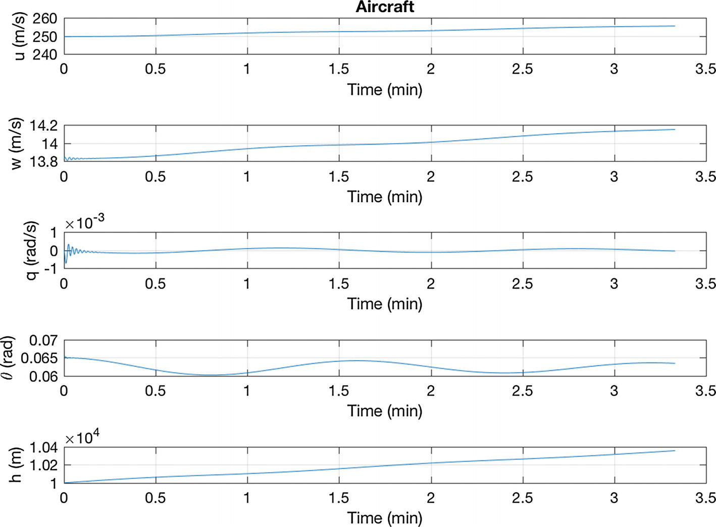
Open loop response to a pulse for the F-16 in a shallow climb.

11.4 Activation Function

11.4.1 Problem

We are going to implement a neural net so that our aircraft control system can learn. We need an activation function to scale and limit measurements.

11.4.2 Solution

Use a sigmoid function as our activation function.

11.4.3 How It Works

The neural net uses the following sigmoid function
$$\displaystyle \begin{aligned} g(x) = \frac{1-e^{-kx}}{1+e^{-kx}} \end{aligned} $$
(11.23)

The sigmoid function with k = 1 is plotted in the following script.

 s = (1- exp (-x))./(1+ exp (-x));
 PlotSet( x, s,  ’x label’,  ’x’,  ’y label’,  ’s’,...
    ’plot title’,  ’Sigmoid’,  ’figure title’,  ’Sigmoid’ );  
Results are shown in Figure 11.4.
../images/420697_2_En_11_Chapter/420697_2_En_11_Fig4_HTML.jpg
Figure 11.4

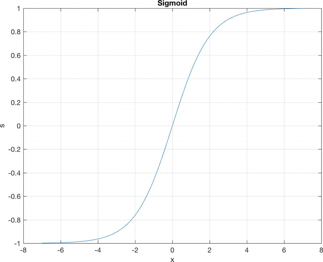
Sigmoid function. At large values of x, the sigmoid function returns ± 1.

11.5 Neural Net for Learning Control

11.5.1 Problem

We want to use a neural net to add learning to the aircraft control system.

11.5.2 Solution

Use a sigma-pi neural net function. A sigma-pi neural net sums the inputs and products of the inputs to produce a model.

11.5.3 How It Works

The adaptive neural network for the pitch axis has seven inputs. The output of the neural network is a pitch angular acceleration that augments the control signal coming from the dynamic inversion controller. The control system is shown in Figure 11.5. The left-most box produces the reference model given the pilot input. The output of the reference model is a vector of the desired states that are differenced with the true states and fed to the PID controller and the neural network. The output of the PID is differenced with the output of the neural network. This is fed into the model inversion block that drives the aircraft dynamics.
../images/420697_2_En_11_Chapter/420697_2_En_11_Fig5_HTML.png
Figure 11.5

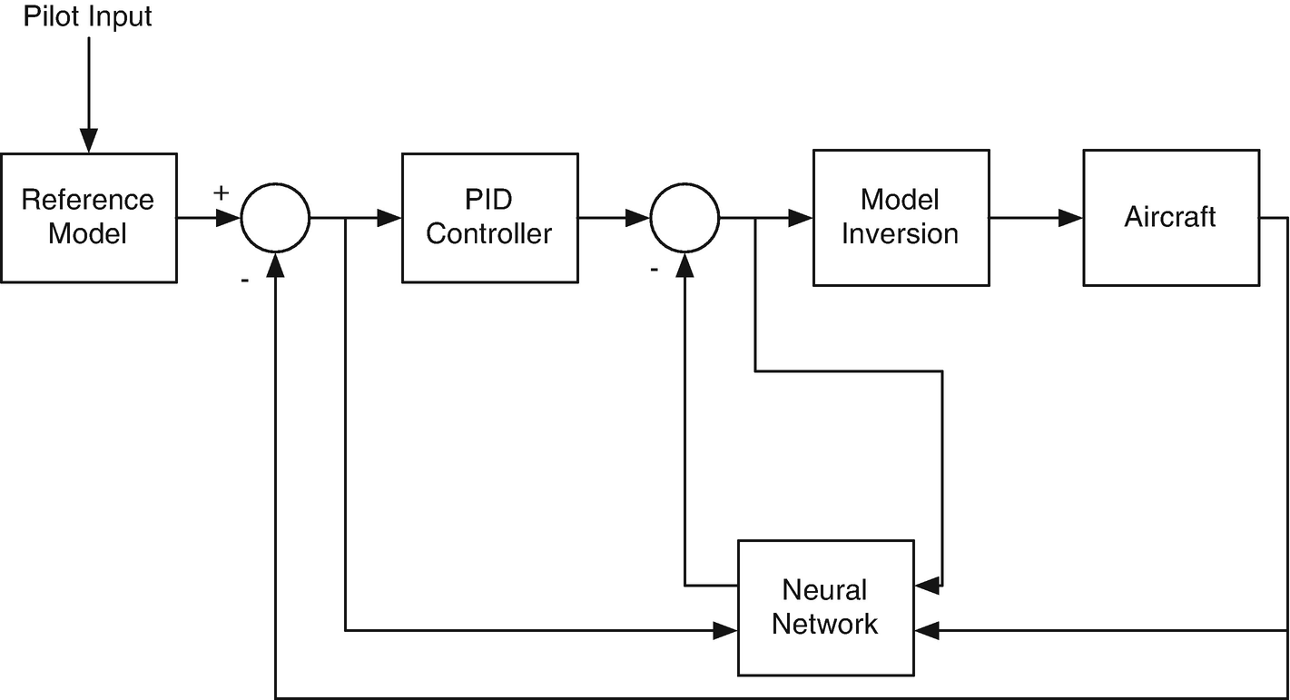
Aircraft control system. It combines a PID controller with dynamic inversion to handle nonlinearities. A neural net provides learning.

The sigma-pi neural net is shown in Figure 11.6 for a two-input system.
../images/420697_2_En_11_Chapter/420697_2_En_11_Fig6_HTML.png
Figure 11.6

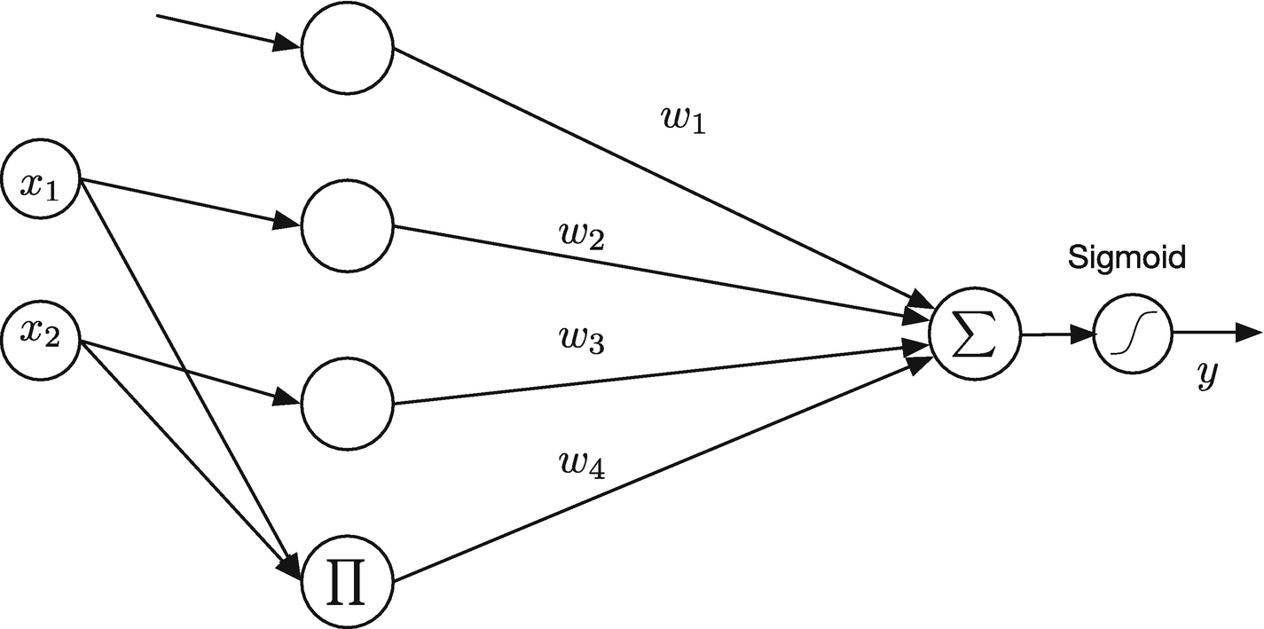
Sigma-pi neural net. Π stands for product and Σ stands for sum.

The output is:
$$\displaystyle \begin{aligned} y = w_1 c + w_2 x_1 + w_3 x_2 + w_4 x_1 x_2 \end{aligned} $$
(11.24)
The weights are selected to represent a nonlinear function. For example, suppose we want to represent the dynamic pressure:
$$\displaystyle \begin{aligned} y = \frac{1}{2}\rho v^2 \end{aligned} $$
(11.25)
We let x 1 = ρ and x 2 = v 2. Set $$w_4 = \frac {1}{2}$$ and all other weights to zero. Suppose we didn’t know the constant $$\frac {1}{2}$$. We would like our neural net to determine the weight through measurements. Learning for a neural net means determining the weights so that our net replicates the function it is modeling. Define the vector z, which is the result of the product operations. In our two-input case this would be:
$$\displaystyle \begin{aligned} z = \left[ \begin{array}{l} c\\ x_1\\ x_2\\ x_1x_2 \end{array} \right] \end{aligned} $$
(11.26)
c is a constant. The output is:
$$\displaystyle \begin{aligned} y = w^Tz \end{aligned} $$
(11.27)
We could assemble multiple inputs and outputs:
$$\displaystyle \begin{aligned} \left[ \begin{array}{lll} y_1&amp;y_2&amp;\cdots \end{array} \right] = w^T\left[ \begin{array}{lll} z_1&amp;z_2&amp;\cdots \end{array} \right] \end{aligned} $$
(11.28)
where zk is a column array. We can solve for the weights w using least squares given the outputs, y, and inputs, x. Define the vector of y to be Y  and the matrix of z to be Z. The solution for w is:
$$\displaystyle \begin{aligned} Y = Z^Tw \end{aligned} $$
(11.29)
The least squares solution is:
$$\displaystyle \begin{aligned} w = \left(ZZ^T\right)^{-1}ZY^T \end{aligned} $$
(11.30)
This gives the best fit to w for the measurements Y  and inputs Z. Suppose we take another measurement. We would then repeat this with bigger matrices. As a side note, you would really compute this using an inverse. There are better numerical methods for doing least squares. MATLAB has the pinv function. For example:
 >> z =  rand (4,4);
 >> w =  rand (4,1);
 >> y = w’*z;
 >> wL =  inv (z*z’)*z*y’
 wL =
     0.8308
     0.5853
     0.5497
     0.9172
 >> w
 w =
     0.8308
     0.5853
     0.5497
     0.9172
 >>  pinv (z’)*y’
ans =
     0.8308
     0.5853
     0.5497
     0.9172  

As you can see, they all agree! This is a good way to initially train your neural net. Collect as many measurements as you have values of z and compute the weights. Your net is then ready to go.

The recursive approach is to initialize the recursive trainer with n values of z and y.
$$\displaystyle \begin{aligned} \begin{array}{rcl} p &amp;\displaystyle =&amp;\displaystyle \left(ZZ^T\right)^{-1} \end{array} \end{aligned} $$
(11.31)
$$\displaystyle \begin{aligned} \begin{array}{rcl} w &amp;\displaystyle =&amp;\displaystyle pZY\vspace{-3pt} \end{array} \end{aligned} $$
(11.32)
The recursive learning algorithm is:
$$\displaystyle \begin{aligned} \begin{array}{rcl} p&amp;\displaystyle =&amp;\displaystyle p - \frac{pzz^Tp}{1+z^Tpz} \end{array} \end{aligned} $$
(11.33)
$$\displaystyle \begin{aligned} \begin{array}{rcl} k &amp;\displaystyle =&amp;\displaystyle pz \end{array} \end{aligned} $$
(11.34)
$$\displaystyle \begin{aligned} \begin{array}{rcl} w &amp;\displaystyle =&amp;\displaystyle w + k\left(y - z^Tw\right)\vspace{-3pt} \end{array} \end{aligned} $$
(11.35)
RecursiveLearning demonstrates recursive learning or training. It starts with an initial estimate based on a four-element training set. It then recursively learns based on new data.
 wN  = w + 0.1* randn (4,1);  % True weights are a little different
 n   = 300;
 zA  =  randn (4,n);  % Random inputs
 y   = wN’*zA;  % 100 new measurements
  % Batch training
 p   =  inv (Z*Z’);  % Initial value
 w   = p*Z*Y;  % Initial value
  %% Recursive learning
 dW =  zeros (4,n);
for j = 1:n
   z       = zA(:,j);
   p       = p - p*(z*z’)*p/(1+z’*p*z);
   w       = w + p*z*(y(j) - z’*w);
   dW(:,j) = w - wN;  % Store for plotting
end
  %% Plot the results
 yL =  cell (1,4);
for j = 1:4
   yL{j} =  sprintf ( ’\\Delta W_%d’,j);
end
 PlotSet(1:n,dW, ’x label’, ’Sample’, ’y label’,yL,...
          ’plot title’, ’Recursive Training’,...
          ’figure title’, ’Recursive Training’);
Figure 11.7 shows the results. After an initial transient, the learning converges. Every time you run this you will get different answers because we initialize with random values.
../images/420697_2_En_11_Chapter/420697_2_En_11_Fig7_HTML.png
Figure 11.7

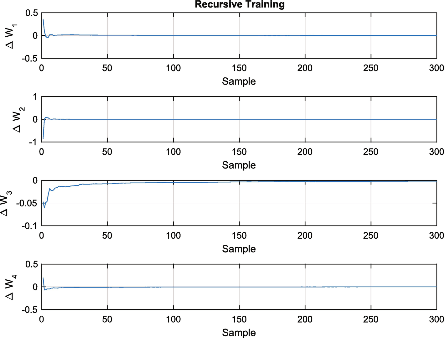
Recursive training or learning. After an initial transient the weights converge quickly.

You will notice that the recursive learning algorithm is identical in form to the Kalman Filter given in Section 4.​1.​3. Our learning algorithm was derived from batch least squares, which is an alternative derivation for the Kalman Filter.

11.6 Enumeration of All Sets of Inputs

11.6.1 Problem

One issue with a sigma-pi neural network is the number of possible nodes. For design purposes, we need a function to enumerate all possible sets of combinations of inputs. This is to determine the limitation of the complexity of a sigma-pi neural network.

11.6.2 Solution

Write a combination function that computes the number of sets.

11.6.3 How It Works

In our sigma-pi network, we hand-coded the products of the inputs. For more general code, we want to enumerate all combinations of inputs. If we have n inputs and want to take them k at a time, the number of sets is:
$$\displaystyle \begin{aligned} \frac{n!}{(n-k)!k!} \end{aligned} $$
(11.36)

The code to enumerate all sets is in the function Combinations.

function c = Combinations( r, k )
  %% Demo
ifnargin < 1 )
   Combinations(1:4,3)
    return
end
  %% Special cases
if( k == 1 )
   c = r’;
    return
elseif( k == length(r) )
   c = r;
    return
end
  %% Recursion
 rJ     = r(2: end );
 c   = [];
iflength(rJ) > 1 )
    for j = 2:length(r)-k+1
     rJ            = r(j: end );
     nC            = NumberOfCombinations( length (rJ),k-1);
     cJ            =  zeros (nC,k);
     cJ(:,2: end )   = Combinations(rJ,k-1);
     cJ(:,1)       = r(j-1);
      if( ~isempty(c) )
       c = [c;cJ];
      else
       c = cJ;
      end
    end
else
   c = rJ;
end
 c = [c;r( end -k+1: end )];

This handles two special cases on input and then calls itself recursively for all other cases. Here are some examples:

 >> Combinations(1:4,3)
ans =
      1     2     3
      1     2     4
      1     3     4
      2     3     4
  >> Combinations(1:4,2)
ans =
      1     2
      1     3
      1     4
      2     3
      2     4
      3     4  

You can see that if we have four inputs and want all possible combinations, we end up with 14 in total! This indicates a practical limit to a sigma-pi neural network, as the number of weights will grow fast as the number of inputs increases.

11.7 Write a Sigma-Pi Neural Net Function

11.7.1 Problem

We need a sigma-pi net function for general problems.

11.7.2 Solution

Use a sigma-pi function.

11.7.3 How It Works

The following code shows how we implement the sigma-pi neural net. SigmaPiNeuralNet has action as its first input. You use this to access the functionality of the function. Actions are:
  1. 1.

    “initialize” – initialize the function

     
  2. 2.

    “set constant” – set the constant term

     
  3. 3.

    “batch learning” – perform batch learning

     
  4. 4.

    “recursive learning” – perform recursive learning

     
  5. 5.

    “output” – generate outputs without training

     
You usually go in order when running the function. Setting the constant is not needed if the default of one is fine.

The functionality is distributed among sub-functions called from the switch statement.

The demo shows an example of using the function to model dynamic pressure. Our inputs are the altitude and the square of the velocity. The neural net will try to fit:
$$\displaystyle \begin{aligned} y = w_1 c+w_2 h + w_3 v^2 + w_4 h v^2 \end{aligned} $$
(11.37)
to
$$\displaystyle \begin{aligned} y =0.6125e^{-0.0817h.^{1.15}}v^2 \end{aligned} $$
(11.38)

We first get a default data structure. Then we initialize the filter with an empty x. We then get the initial weights by using batch learning. The number of columns of x should be at least twice the number of inputs. This gives a starting p matrix and initial estimate of weights. We then perform recursive learning. It is important that the field kSigmoid is small enough so that valid inputs are in the linear region of the sigmoid function. Note that this can be an array so that you can use different scalings on different inputs.

function Demo
  % Demonstrate a sigma-pi neural net for dynamic pressure
 x       =  zeros (2,1);
 d       = SigmaPiNeuralNet;
 [~, d]  = SigmaPiNeuralNet(  ’initialize’, x, d );
 h       =  linspace (10,10000);
 v       =  linspace (10,400);
 v2      = v.^2;
 q       = 0.5*AtmDensity(h).*v2;
 n       = 5;
 x       = [h(1:n);v2(1:n)];
 d.y     = q(1:n)’;
 [y, d]  = SigmaPiNeuralNet(  ’batch learning’, x, d );
fprintf(1, ’Batch Results\n#         Truth   Neural Net\n’);
for k = 1:length(y)
    fprintf(1, ’%d: %12.2f %12.2f\n’,k,q(k),y(k));
end
 n =  length (h);
 y =  zeros (1,n);
 x = [h;v2];
for k = 1:n
   d.y = q(k);
   [y(k), d]  = SigmaPiNeuralNet(  ’recursive learning’, x(:,k), d );
end

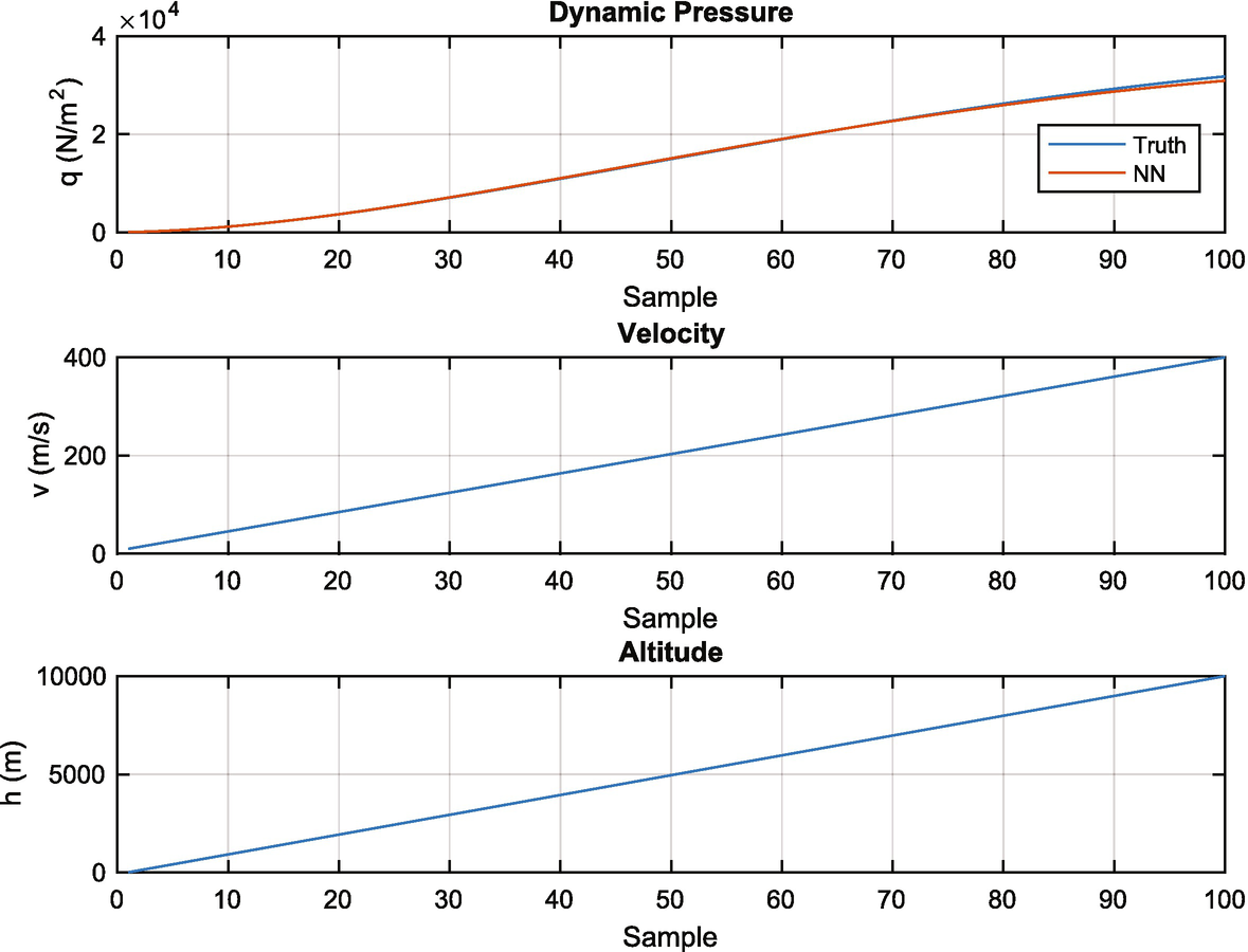
The batch results are as follows for five examples of dynamic pressures at low altitude. As you can see the truth model and neural net outputs are quite close:

 >> SigmaPiNeuralNet
 Batch Results
 #         Truth   Neural Net
 1:        61.22        61.17
 2:       118.24       118.42
 3:       193.12       192.88
 4:       285.38       285.52
 5:       394.51       394.48  

The recursive learning results are shown in Figure 11.8. The results are pretty good over a wide range of altitudes. You could then just use the “update” action during aircraft operation.

11.8 Implement PID Control

11.8.1 Problem

We want a PID controller to control the aircraft.

11.8.2 Solution

Write a function to implement PID control. The inputs will be the pitch angle error.
../images/420697_2_En_11_Chapter/420697_2_En_11_Fig8_HTML.png
Figure 11.8

Recursive training for the dynamic pressure example.

11.8.3 How It Works

Assume we have a double integrator driven by a constant input:
$$\displaystyle \begin{aligned} \ddot{x}= u \end{aligned} $$
(11.39)
where u = ud + uc.
The result is:
$$\displaystyle \begin{aligned} x = \frac{1}{2}ut^2 + x(0) + \dot{x}(0)t \end{aligned} $$
(11.40)
The simplest control is to add a feedback controller
$$\displaystyle \begin{aligned} u_c = - K \left(\tau_d\dot{x} + x\right) \end{aligned} $$
(11.41)
where K is the forward gain and τ is the damping time constant. Our dynamical equation is now:
$$\displaystyle \begin{aligned} \ddot{x} + K \left(\tau_d\dot{x} + x\right) = u_d \end{aligned} $$
(11.42)
The damping term will cause the transients to die out. When that happens, the second derivative and first derivatives of x are zero and we end up with an offset:
$$\displaystyle \begin{aligned} x = \frac{u}{K} \end{aligned} $$
(11.43)
This is generally not desirable. You could increase K until the offset were small, but that would mean your actuator would need to produce higher forces or torques. What we have at the moment is a proportional derivative (PD) controller. Let’s add another term to the controller:
$$\displaystyle \begin{aligned} u_c = - K \left(\tau_d\dot{x} + x+ \frac{1}{\tau_i}\int x\right) \end{aligned} $$
(11.44)
This is now a proportional integral derivative (PID) controller. There is now a gain proportional to the integral of x. We add the new controller, and then take another derivative to get:
$$\displaystyle \begin{aligned} \dddot{x} + K \left(\tau_d\ddot{x} + \dot{x} + \frac{1}{\tau_i}x\right) = \dot{u}_d \end{aligned} $$
(11.45)
Now in steady state:
$$\displaystyle \begin{aligned} x = \frac{\tau_i}{K}\dot{u}_d \end{aligned} $$
(11.46)
If u is constant, the offset is zero. Define s as the derivative operator.
$$\displaystyle \begin{aligned} s = \frac{d}{dt} \end{aligned} $$
(11.47)
Then:
$$\displaystyle \begin{aligned} s^3x(s) + K \left(\tau_ds^2x(s) + sx(s) + \frac{1}{\tau_i}x(s)\right) = su_d(s) \end{aligned} $$
(11.48)
Note that:
$$\displaystyle \begin{aligned} \frac{u_c(s)}{x(s)} = K\left(1 + \tau_d s + \frac{1}{\tau_i s}\right) \end{aligned} $$
(11.49)
where τd is the rate time constant, which is how long the system will take to damp and τi is how fast the system will integrate out a steady disturbance.
where s =  and $$j = \sqrt {-1}$$. The closed loop transfer function is:
$$\displaystyle \begin{aligned} \begin{array}{rcl} \frac{x(s)}{u_d(s)} = \frac{s}{s^3 + K\tau_ds^2 + Ks + K/\tau_i} \end{array} \end{aligned} $$
(11.50)
The desired closed loop transfer function is:
$$\displaystyle \begin{aligned} \begin{array}{rcl} \frac{x(s)}{u_d(s)} = \frac{s}{(s + \gamma)(s^2+2\zeta\sigma s + \sigma^2)} \end{array} \end{aligned} $$
(11.51)
or
$$\displaystyle \begin{aligned} \begin{array}{rcl} \frac{x(s)}{u_d(s)} = \frac{s}{s^3 + (\gamma + 2\zeta\sigma)s^2 + \sigma(\sigma + 2\zeta\gamma)s + \gamma\sigma^2} \end{array} \end{aligned} $$
(11.52)
The parameters are:
$$\displaystyle \begin{aligned} \begin{array}{rcl} K &amp;\displaystyle =&amp;\displaystyle \sigma(\sigma + 2\zeta\gamma) \end{array} \end{aligned} $$
(11.53)
$$\displaystyle \begin{aligned} \begin{array}{rcl} \tau_i &amp;\displaystyle =&amp;\displaystyle \frac{\sigma + 2\zeta\gamma}{\gamma\sigma} \end{array} \end{aligned} $$
(11.54)
$$\displaystyle \begin{aligned} \begin{array}{rcl} \tau_d &amp;\displaystyle =&amp;\displaystyle \frac{\gamma + 2\zeta\sigma}{ \sigma(\sigma + 2\zeta\gamma)}\vspace{-2pt} \end{array} \end{aligned} $$
(11.55)
This is a design for a PID. However, it is not possible to write this in the desired state space form:
$$\displaystyle \begin{aligned} \begin{array}{rcl} \dot{x} &amp;\displaystyle =&amp;\displaystyle Ax + Au \end{array} \end{aligned} $$
(11.56)
$$\displaystyle \begin{aligned} \begin{array}{rcl} y &amp;\displaystyle =&amp;\displaystyle Cx + Du\vspace{-2pt} \end{array} \end{aligned} $$
(11.57)
because it has a pure differentiator. We need to add a filter to the rate term so that it looks like:
$$\displaystyle \begin{aligned} \frac{s}{\tau_rs + 1}\end{aligned} $$
(11.58)
instead of s. We aren’t going to derive the constants and will leave it as an exercise for the reader. The code for the PID is in PID.
function [a, b, c, d] = PID(  zeta, omega, tauInt, omegaR, tSamp )
  % Demo
ifnargin < 1 )
   Demo;
    return
end
  % Input processing
ifnargin < 4 )
   omegaR = [];
end
  % Default roll-off
ifisempty(omegaR) )
   omegaR = 5*omega;
end
  % Compute the PID gains
 omegaI  = 2* pi /tauInt;
 c2  = omegaI*omegaR;
 c1  = omegaI+omegaR;
 b1  = 2*zeta*omega;
 b2  = omega^2;
 g   = c1 + b1;
 kI  = c2*b2/g;
 kP  = (c1*b2 + b1.*c2  - kI)/g;
 kR  = (c1*b1 + c2 + b2 - kP)/g;
  % Compute the state space model
 a   =  [0 0;0 -g];
 b   =  [1;g];
 c   =  [kI -kR*g];
 d   =  kP + kR*g;
  % Convert to discrete time
ifnargin > 4 )
   [a,b] = CToDZOH(a,b,tSamp);
end
It is interesting to evaluate the effect of the integrator. This is shown in Figure 11.9. The code is the demo in PID. Instead of numerically integrating the differential equations we convert them into sampled time and propagate them. This is handy for linear equations. The double integrator equations are in the form:
$$\displaystyle \begin{aligned} \begin{array}{rcl} x_{k+1} &amp;\displaystyle =&amp;\displaystyle a x_k + b u_k \end{array} \end{aligned} $$
(11.59)
$$\displaystyle \begin{aligned} \begin{array}{rcl} y &amp;\displaystyle =&amp;\displaystyle c x_k + d u_k\vspace{-3pt} \end{array} \end{aligned} $$
(11.60)
This is the same form as the PID controller.
../images/420697_2_En_11_Chapter/420697_2_En_11_Fig9_HTML.png
Figure 11.9

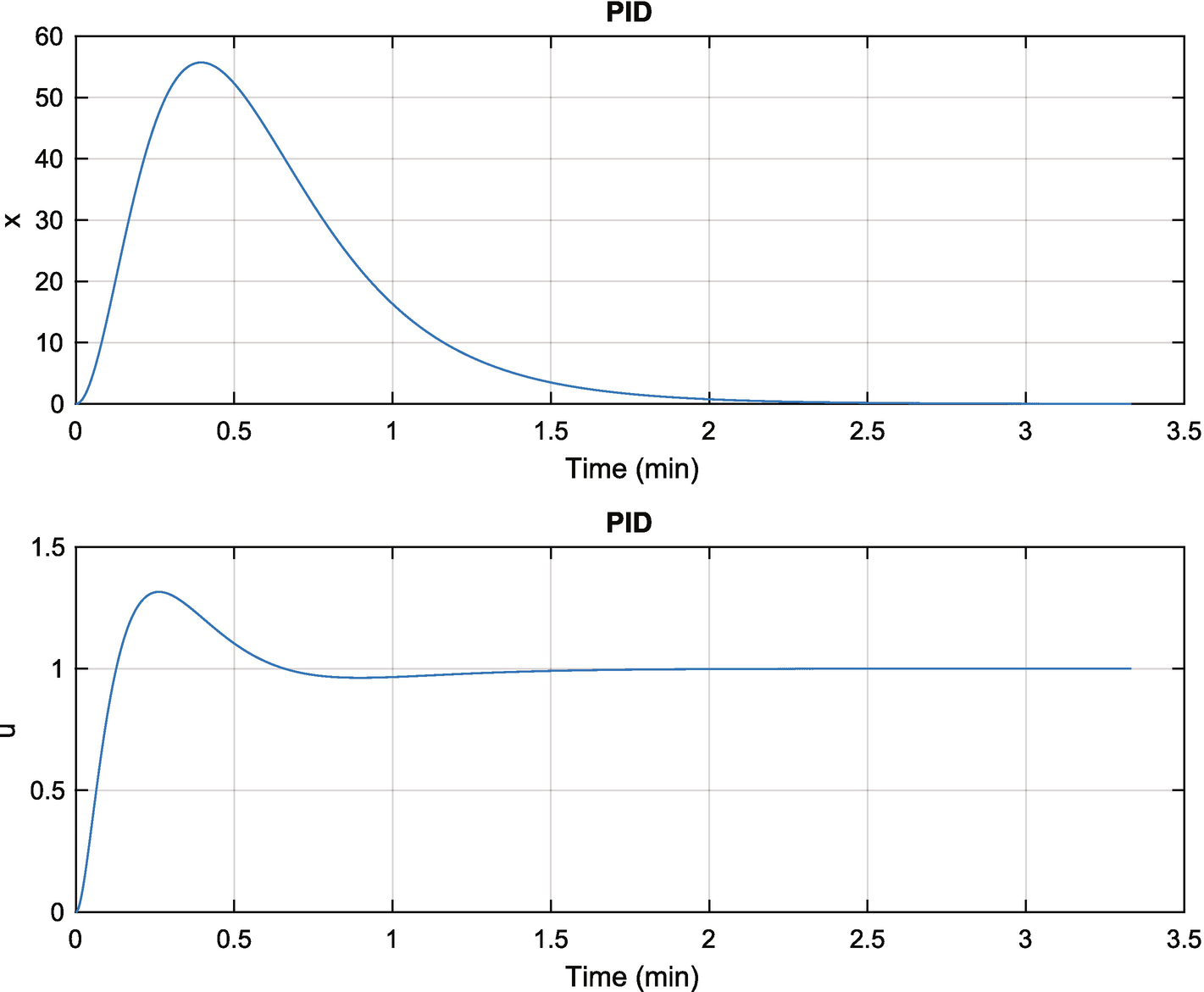
Proportional integral derivative control given a unit input.

  % The double integrator plant
 dT            = 0.1;  % s
 aP            = [0 1;0 0];
 bP            = [0;1];
 [aP, bP]      = CToDZOH( aP, bP, dT );
  % Design the controller
 [a, b, c, d]  = PID(  1, 0.1, 100, 0.5, dT );
  % Run the simulation
 n   = 2000;
 p   =  zeros (2,n);
 x   = [0;0];
 xC  = [0;0];
for k = 1:n
    % PID Controller
   y       = x(1);
   xC      = a*xC + b*y;
   uC      = c*xC + d*y;
   p(:,k)  = [y;uC];
   x       = aP*x + bP*(1-uC);  % Unit step response
end

It takes about 2 minutes to drive x to zero, which is close to the 100 seconds specified for the integrator.

11.9 PID Control of Pitch

11.9.1 Problem

We want to control the pitch angle of an aircraft with a PID controller.

11.9.2 Solution

Write a script to implement the controller with the PID controller and pitch dynamic inversion compensation.

11.9.3 How It Works

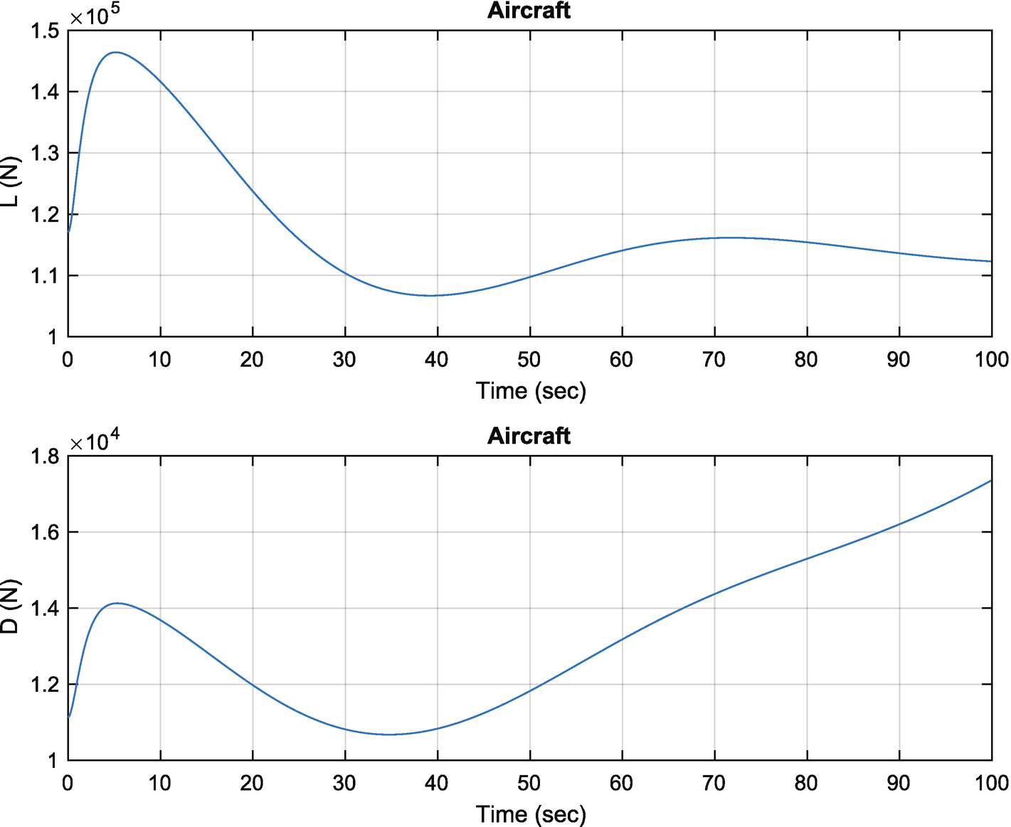
The PID controller changes the elevator angle to produce a pitch acceleration to rotate the aircraft. The elevator is the moveable horizontal surface that is usually on the tail wing of an aircraft. In addition, additional elevator movement is needed to compensate for changes in the accelerations due to lift and drag as the aircraft changes its pitch orientation. This is done using the pitch dynamic inversion function. This returns the pitch acceleration, which must be compensated for when applying the pitch control.

function qDot = PitchDynamicInversion( x, d )
ifnargin < 1 )
   qDot = DataStructure;
    return
end
 u     = x(1);
 w     = x(2);
 h     = x(5);
 rho   = AtmDensity( h );
 alpha =  atan (w/u);
 cA    =  cos (alpha);
 sA    =  sin (alpha);
 v     =  sqrt (u^2 + w^2);
 pD    = 0.5*rho*v^2;  % Dynamic pressure
 cL    = d.cLAlpha*alpha;
 cD    = d.cD0 + d.k*cL^2;
 drag  = pD*d.s*cD;
 lift  = pD*d.s*cL;
 z     = -lift*cA - drag*sA;
 m     = d.c*z;
 qDot  = m/d.inertia;  
The simulation incorporating the controls is AircraftSim below. There is a flag to turn on control and another to turn on the learning control. We command a 0.2-radian pitch angle using the PID control. The results are shown in Figure 11.10, Figure 11.11 and Figure 11.12.
../images/420697_2_En_11_Chapter/420697_2_En_11_Fig10_HTML.png
Figure 11.10

Aircraft pitch angle change. The aircraft oscillates because of the pitch dynamics.

The maneuver increases the drag and we don’t adjust the throttle to compensate. This will cause the airspeed to drop. In implementing the controller we neglected to consider coupling between states, but this can be added easily.

11.10 Neural Net for Pitch Dynamics

11.10.1 Problem

We want a nonlinear inversion controller with a PID controller and the sigma-pi neural net.

11.10.2 Solution

Train the neural net with a script that takes the angle and velocity squared input and computes the pitch acceleration error.

11.10.3 How It Works

The PitchNeuralNetTraining script computes the pitch acceleration for a slightly different set of parameters. It then processes the delta-acceleration. The script passes a range of pitch angles to the function and learns the acceleration. We use the velocity squared as an input because the dynamic pressure is proportional to the velocity squared. The base acceleration (in dRHSL) is for our “a-priori” model. dRHS is the measured values. We assume that these are obtained during flight testing.
../images/420697_2_En_11_Chapter/420697_2_En_11_Fig11_HTML.png
Figure 11.11

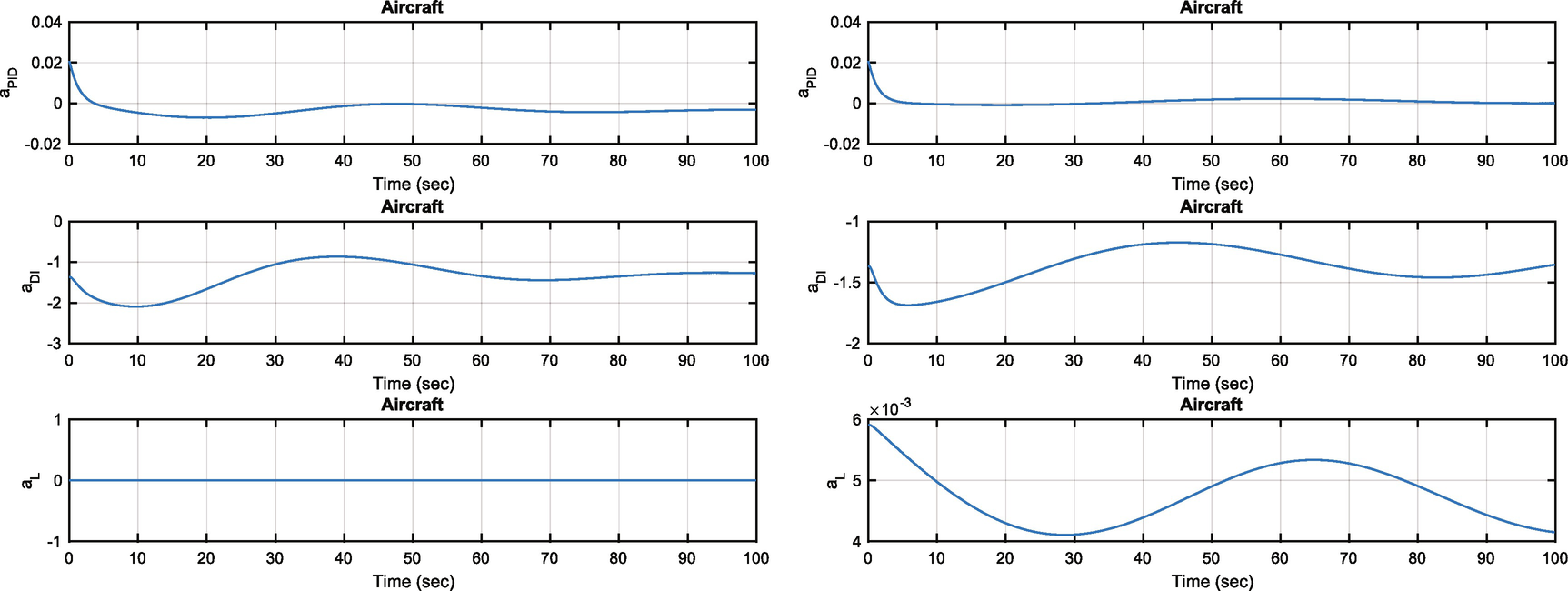
Aircraft pitch angle change. Notice the changes in lift and drag with angle.

../images/420697_2_En_11_Chapter/420697_2_En_11_Fig12_HTML.png
Figure 11.12

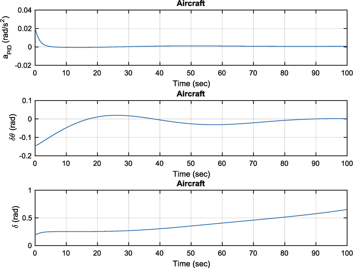
Aircraft pitch angle change. The PID acceleration is much lower than the pitch inversion acceleration.

  % This is from flight testing
 dRHS  = RHSAircraft;    % Get the default data structure has F-16 data
 h  = 10000;
 gamma         = 0.0;
 v             = 250;
  % Get the equilibrium state
 [x,  dRHS.thrust, deltaEq, cost] = EquilibriumState( gamma, v, h, dRHS );
  % Angle of attack
 alpha         =  atan (x(2)/x(1));
 cA            =  cos (alpha);
 sA            =  sin (alpha);
  % Create the assumed properties
 dRHSL         = dRHS;
 dRHSL.cD0     = 2.2*dRHS.cD0;
 dRHSL.k       = 1.0*dRHSL.k;
  % 2 inputs
 xNN     =  zeros (2,1);
 d       = SigmaPiNeuralNet;
 [~, d]  = SigmaPiNeuralNet(  ’initialize’, xNN, d );
 theta   =  linspace (0, pi /8);
 v       =  linspace (300,200);
 n       =  length (theta);
 aT      =  zeros (1,n);
 aM      =  zeros (1,n);
for k   = 1:n
   x(4)  = theta(k);
   x(1)  = cA*v(k);
   x(2)  = sA*v(k);
   aT(k) = PitchDynamicInversion( x, dRHSL );
   aM(k) = PitchDynamicInversion( x, dRHS  );
end
  % The delta pitch acceleration
 dA        = aM - aT;
  % Inputs to the neural net
 v2        = v.^2;
 xNN       = [theta;v2];
  % Outputs for training
 d.y       = dA’;
 [aNN, d]  = SigmaPiNeuralNet(  ’batch learning’, xNN, d );
  % Save the data for the aircraft simulation
 thisPath = fileparts(mfilename( ’fullpath’));
save( fullfile(thisPath, ’DRHSL’), ’dRHSL’ );
save( fullfile(thisPath, ’DNN’),  ’d’  );
for j = 1:size(xNN,2)
   aNN(j,:) = SigmaPiNeuralNet(  ’output’, xNN(:,j), d );
end
  % Plot the results  

The script first finds the equilibrium state using EquilibriumState. It then sets up the sigma-pi neural net using SigmaPiNeuralNet. PitchDynamicInversion is called twice, once to get the model aircraft acceleration aM (the way we want the aircraft to behave) and once to get the true acceleration aT. The delta acceleration, dA is used to train the neural net. The neural net produces aNN. The resulting weights are saved in a .mat file for use in AircraftSim. The simulation uses dRHS, but our pitch acceleration model uses dRHSL. The latter is saved in another .mat file.

 >> PitchNeuralNetTraining
 Velocity            250.00 m/s
 Altitude          10000.00 m
 Flight path angle     0.00 deg
 Z speed              13.84 m/s
 Thrust            11148.95 N
 Angle of attack       3.17 deg
 Elevator             11.22 deg
 Initial cost      9.62e+01
 Final cost        1.17e-17  

As can be seen, the neural net reproduces the model very well. The script also outputs DNN. mat, which contains the trained neural net data.

11.11 Nonlinear Simulation

11.11.1 Problem

We want to demonstrate our learning control system for controlling the longitudinal dynamics of an aircraft.
../images/420697_2_En_11_Chapter/420697_2_En_11_Fig13_HTML.png
Figure 11.13

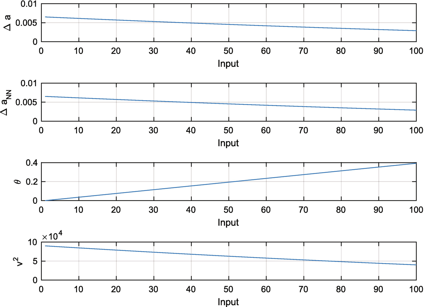
Neural net fitted to the delta acceleration.

11.11.2 Solution

Enable the control functions to the simulation script described in AircraftSimOpenLoop.

11.11.3 How It Works

After training, the neural net in the previous recipe we set addLearning to true. The weights are read in. We command a 0.2-radian pitch angle using the PID learning control. The results are shown in Figure 11.14, Figure 11.15, and Figure 11.16. The figures show without learning control on the left and with learning control on the right.
../images/420697_2_En_11_Chapter/420697_2_En_11_Fig14_HTML.png
Figure 11.14

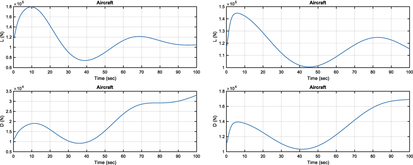
Aircraft pitch angle change. Lift and drag variations are shown.

../images/420697_2_En_11_Chapter/420697_2_En_11_Fig15_HTML.png
Figure 11.15

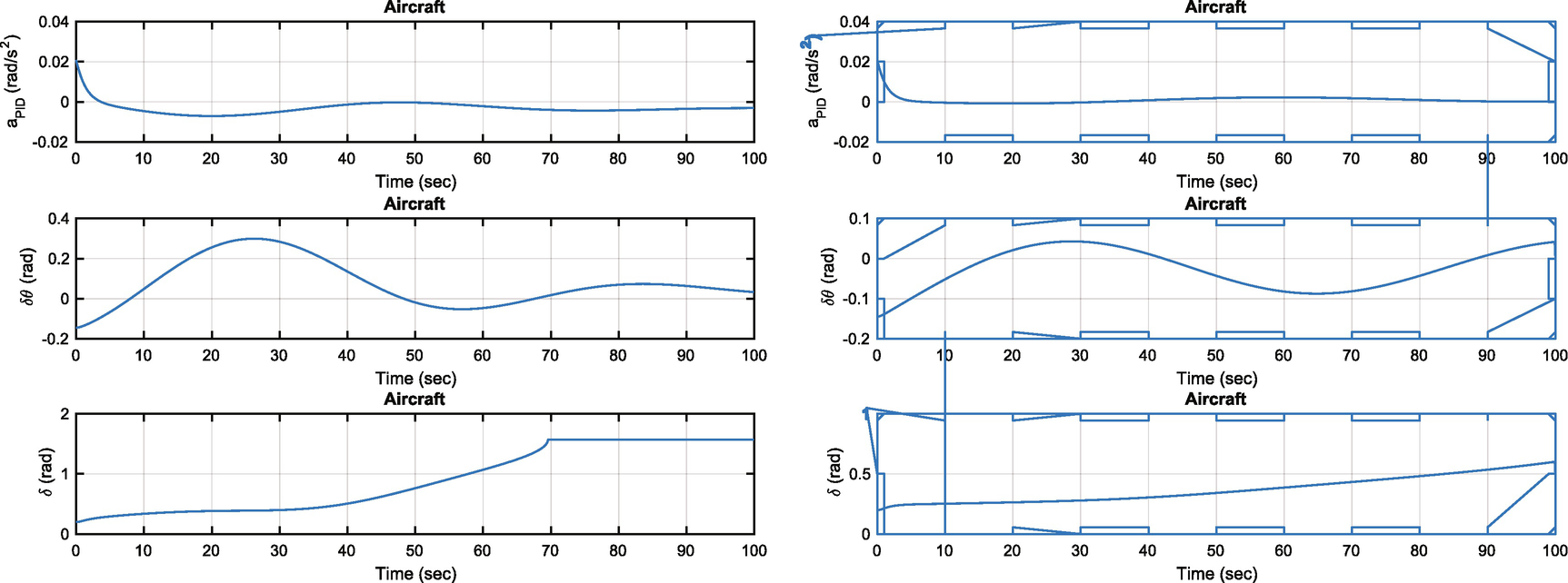
Aircraft pitch angle change. Without learning control, the elevator saturates.

../images/420697_2_En_11_Chapter/420697_2_En_11_Fig16_HTML.png
Figure 11.16

Aircraft pitch angle change. The PID acceleration is much lower than the pitch dynamic inversion acceleration.

Learning control helps the performance of the controller. However, the weights are fixed throughout the simulation. Learning occurs prior to the controller becoming active. The control system is still sensitive to parameter changes since the learning part of the control was computed for a pre-determined trajectory. Our weights were determined only as a function of pitch angle and velocity squared. Additional inputs would improve the performance. There are many opportunities for you to try to expand and improve the learning system.

11.12 Summary

This chapter has demonstrated adaptive or learning control for an aircraft. You learned about model tuning, model reference adaptive control, adaptive control, and gain scheduling. You also learned how to use a neural net as part of an aircraft control system. Table 11.3 lists the functions and scripts included in the companion code.
Table 11.3

Chapter Code Listing

File

Description

AircraftSim

Simulation of the longitudinal dynamics of an aircraft.

AtmDensity

Atmospheric density using a modified exponential model.

EquilibriumState

Finds the equilibrium state for an aircraft.

PID

Implements a PID controller.

PitchDynamicInversion

Pitch angular acceleration.

PitchNeuralNetTraining

Train the pitch acceleration neural net.

QCR

Generates a full state feedback controller.

RecursiveLearning

Demonstrates recursive neural net training or learning.

RHSAircraft

Right-hand side for aircraft longitudinal dynamics.

SigmaPiNeuralNet

Implements a sigma-pi neural net.

Sigmoid

Plots a sigmoid function.