© Michael Paluszek and Stephanie Thomas  2019
Michael Paluszek and Stephanie ThomasMATLAB Machine Learning Recipeshttps://doi.org/10.1007/978-1-4842-3916-2_7

7. Data Classification with Decision Trees

Michael Paluszek1  and Stephanie Thomas1
(1)
Plainsboro, NJ, USA
 

In this chapter, we will develop the theory for binary decision trees. Decision trees can be used to classify data, and fall into the Learning category in our Autonomous Learning taxonomy. Binary trees are easiest to implement because each node branches to two other nodes, or none. We will create functions for the Decision Trees and to generate sets of data to classify. Figure 7.1 shows a simple binary tree. Point “a” is in the upper left quadrant. The first binary test finds that its x value is greater than 1. The next test finds that its y value is greater than 1 and puts it in set 2. Although the boundaries show square regions, the binary tree really tests for regions that go to infinity in both x and y.

../images/420697_2_En_7_Chapter/420697_2_En_7_Figa_HTML.gif

A binary decision tree is a decision tree in which at each decision node there are only two decisions to make. Once you make a decision, the next decision node provides you with two additional options. Each node accepts a binary value of 0 or 1. 0 sends you down one path, and 1 the other. At each decision node, you are testing a new variable. When you get to the bottom, you will have found a path where all of the values are true. The problem with a binary tree of n variables is that it will have 2n − 1 nodes. Four variables would require 15 decision nodes. Eight would require 65 decision nodes, and so forth. If the order of testing variables is fixed, we call it an ordered tree.
../images/420697_2_En_7_Chapter/420697_2_En_7_Fig1_HTML.png
Figure 7.1

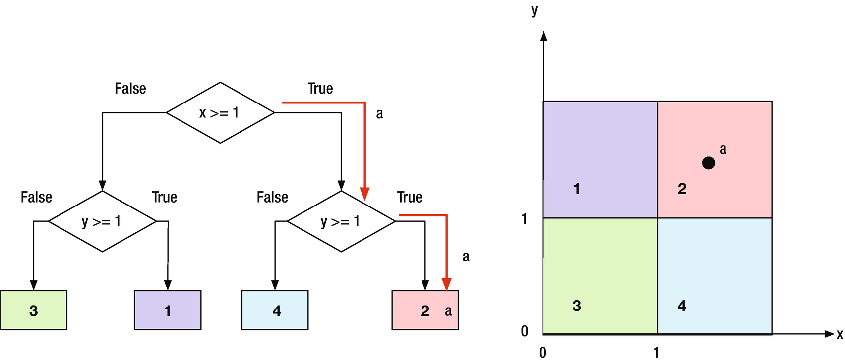
A simple binary tree with one point to classify.

For classification, we are assuming that we can make a series of binary decisions to classify something. If we can, we can implement the reasoning in a binary tree.

7.1 Generate Test Data

7.1.1 Problem

We want to generate a set of training and testing data for classification.

7.1.2 Solution

Write a function using rand to generate data over a selected range in two dimensions, x and y.

7.1.3 How It Works

The function ClassifierSet generates random data and assigns them to classes. The function call is:

function p = ClassifierSets( n, xRange, yRange, name, v, f, setName )  

The first argument to ClassifierSets is the square root of the number of points. The second, xRange, gives the x range for the data and the third, yRange, gives the y range. The n 2 points will be placed randomly in this region. The next argument is a cell array with the names of the sets, name. These are used for plot labels. The remaining inputs are a list of vertices, v, and the faces, f. The faces select the vertices to use in each polygon. The faces connect the vertices into specific polygons. f is a cell array, since each face array can be of any length. A triangle has a length of 3, a hexagon a length of 6. Triangles, rectangles, and hexagons can be easily meshed so that there are no gaps.

Classes are defined by adding polygons that divide the data into regions. Any polygon can be used. You should pick polygons so that there are no gaps. Rectangles are easy, but you could also use uniformly sized hexagons. The following code is the built-in demo. The demo is the last subfunction in the function. This specifies the vertices and faces.

function Demo
 v = [0 0;0 4; 4 4; 4 0; 0 2; 2 2; 2 0;2 1;4 1;2 1];
 f = {[5 6 7 1] [5 2 3 9 10 6] [7 8 9 4]};
 ClassifierSets( 5, [0 4], [0 4], { ’width’,  ’length’}, v, f );

In this demo, there are three polygons. All points are defined in a square ranging from 0 to 4 in both the x and y directions.

The other subfunctions are PointInPolygon and Membership. Membership determines if a point is in a polygon. Membership calls PointInPolygon to assign points to sets. ClassifierSets randomly puts points in the regions. It figures out which region each point is in using this code in the function, PointInPolygon.

function r = PointInPolygon( p, v )
 m =  size (v,2);
  % All outside
 r = 0;
  % Put the first point at the end to simplify the looping
 v = [v v(:,1)];
for i = 1:m
   j   = i + 1;
   v2J   = v(2,j);
   v2I = v(2,i);
    if (((v2I > p(2)) ~= (v2J > p(2))) && ...
       (p(1) < (v(1,j) - v(1,i)) * (p(2) - v2I) / (v2J - v2I) + v(1,i)))
     r = ~r;
    end
end

This code can determine if a point is inside a polygon defined by a set of vertices. It is used frequently in computer graphics and in games when you need to know if one object’s vertex is in another polygon. You could correctly argue that this function could replace our decision tree logic for this type of problem. However, a decision tree can compute membership for more complex sets of data. Our classifier set is simple and makes it easy to validate the results.

Run ClassifierSets to see the demo. Given the input ranges, it determines the membership of randomly selected points. p is a data structure that holds the vertices and the membership. It plots the points after creating a new figure using NewFigure. It then uses patch to create the rectangular regions.

 p.x    = (xRange(2) - xRange(1))*( rand (n,n)-0.5) +  mean (xRange);
 p.y    = (yRange(2) - yRange(1))*( rand (n,n)-0.5) +  mean (yRange);
 p.m    = Membership( p, v, f );
 NewFigure(setName);
 i = 0;
 drawNum = n^2 < 50;
for j = 1:n
    for k = 1:n
     i = i + 1;
      plot(p.x(k,j),p.y(k,j), ’marker’, ’o’, ’MarkerEdgeColor’, ’k’)
      if( drawNum )
        text(p.x(k,j),p.y(k,j),sprintf( ’ %3d’,i));
      end
      hold on
    end
end
 m =  length (f);
 a =  linspace (0,2* pi -2* pi /m,m)’;
 c =  abs ( cos ([a a+ pi /6 a+3* pi /5]));
for k = 1:m
    patch( ’vertices’,v, ’faces’,f{k}, ’facecolor’,c(k,:), ’facealpha’,0.1)
end
xlabel(name{1});
ylabel(name{2});
grid on

The function shows the data numbers if there are fewer than 50 points. The MATLAB-function patch is used to generate the polygons. The code shows a range of graphics coding including the use of graphics parameters. Notice the way we create m colors.

TIP

You can create an unlimited number of colors for plots using linspace and cos.

../images/420697_2_En_7_Chapter/420697_2_En_7_Fig2_HTML.png
Figure 7.2

Classifier set with three regions from the demo. Two are rectangles and one is L-shaped.

ClassifierTestSet can generate test sets or demonstrate a trained decision tree. The drawing shows that the classification regions are regions with sides parallel to the x- or y-axes. The regions should not overlap.

7.2 Drawing Decision Trees

7.2.1 Problem

We want to draw a binary decision tree to show decision tree thinking.

7.2.2 Solution

The solution is to use MATLAB graphics functions, patch, text, and line to draw a tree.

7.2.3 How It Works

The function DrawBinaryTree draws any binary tree. The function call is

function d = DrawBinaryTree( d, name )  
You pass it a data structure, d, with the decision criteria in a cell array. The name input is optional. It has a default option for the name. The boxes start from the left and go row by row. In a binary tree, the number of rows is related to the number of nodes through the formula for a geometric series:
$$\displaystyle \begin{aligned} m = \log_2(n) \end{aligned} $$
(7.1)
where m is the number of rows and n is the number of boxes. Therefore, the function can compute the number of rows.

The function starts by checking the number of inputs and either runs the demo or returns the default data structure. When you write a function you should always have defaults for anything where one is possible.

TIP

Whenever possible, have default inputs for function arguments.

It immediately creates a new figure with that name. It then steps through the boxes assigning them to rows based on it being a binary tree. The first row has one box, the next two boxes, the following four boxes, etc. As this is a geometric series, it will soon get unmanageable! This points to a problem with decision trees. If they have a depth of more than four, even drawing them is impossible. As it draws the boxes, it computes the bottom and top points, which will be the anchors for the lines between the boxes. After drawing all the boxes, it draws all the lines.

All of the drawing functionality is in the subfunction DrawBox.

 v = [x y 0;x y+h 0; x+w y+h 0;x+w y 0];
patch( ’vertices’,v, ’faces’,[1 2 3 4], ’facecolor’,[1;1;1]);
text(x+w/2,y + h/2,t, ’fontname’,d.font, ’fontsize’,...
   d.fontSize, ’HorizontalAlignment’, ’center’);
  %% DrawBinaryTree>DefaultDataStructure  

This draws a box using the patch function and the text using the text function. ’facecolor’ is white. Red green blue (RGB) numbers go from 0 to 1. Setting ’facecolor’ to [1 1 1] makes the face white and leaves the edges black. As with all MATLAB graphics, there are dozens of properties that you can edit to produce beautiful graphics. Notice the extra arguments in text. The most interesting is ’HorizontalAlignment’ in the last line. It allows you to center the text in the box. MATLAB does all the figuring of font sizes for you.

The following listing shows the code in DrawBinaryTree, for drawing the tree, starting after checking for demos. The function returns the default data structure if one output and no inputs are specified. The first part of the code creates a new figure and draws the boxes at each node. It also creates arrays for the box locations for use in drawing the lines that connect the boxes. It starts off with the default argument for name. The first set of loops draws the boxes for the trees. rowID is a cell array. Each row in the cell is an array. A cell array allows each cell to be different. This makes it easy to have different length arrays in the cell. If you used a standard matrix, you would need to resize rows as new rows were added.

ifnargin < 2 )
   name =  ’Binary Tree’;
end
 NewFigure(name);
 m       =  length (d.box);
 nRows   =  ceil ( log2 (m+1));
 w       = d.w;
 h       = d.h;
 i       = 1;
 x       = -w/2;
 y       =  1.5*nRows*h;
 nBoxes  = 1;
 bottom  =  zeros (m,2);
 top     =  zeros (m,2);
 rowID   =  cell (nRows,1);
  % Draw a box at each node
for k = 1:nRows
    for j = 1:nBoxes
     bottom(i,:)   = [x+w/2 y ];
     top(i,:)      = [x+w/2 y+h];
     DrawBox(d.box{i},x,y,w,h,d);
     rowID{k}      = [rowID{k} i];
     i             = i + 1;
     x             = x + 1.5*w;
      if( i > length(d.box) )
        break;
      end
    end
   nBoxes  = 2*nBoxes;
   x       = -(0.25+0.5*(nBoxes/2-1))*w - nBoxes*w/2;
   y       = y - 1.5*h;
end

The remaining code draws the lines between the boxes.

for k = 1:length(rowID)-1
   iD = rowID{k};
   i0 = 0;
    % Work from left to right of the current row
    for j = 1:length(iD)
     x(1) = bottom(iD(j),1);
     y(1) = bottom(iD(j),2);
     iDT  = rowID{k+1};
      if( i0+1 > length(iDT) )
        break;
      end
      for i = 1:2
       x(2) = top(iDT(i0+i),1);
       y(2) = top(iDT(i0+i),2);
        line(x,y);
      end
     i0 = i0 + 2;
    end
end
axis off  

The following built-in demo draws a binary tree. The demo creates three rows. It starts with the default data structure. You only have to add strings for the decision points. The boxes are in a flat list.

function Demo
  % Draw a simple binary data treea
 d           = DefaultDataStructure;
 d.box{1}    =  ’a > 0.1’;
 d.box{2}    =  ’b > 0.2’;
 d.box{3}    =  ’b > 0.3’;
 d.box{4}    =  ’a > 0.8’;
 d.box{5}    =  ’b > 0.4’;
 d.box{6}    =  ’a > 0.2’;
 d.box{7}    =  ’b > 0.3’;
 DrawBinaryTree( d );  

Notice that it calls the subfunction DefaultDataStructure to initialize the demo.

  %% DrawBinaryTree>DefaultDataStructure
function d = DefaultDataStructure
  % Default data structure
 d           = struct();
 d.fontSize  = 12;
 d.font      =  ’courier’;
 d.w         = 1;
 d.h         = 0.5;
 d.box       = {};  

TIP

Always have the function return its default data structure. The default should have values that work.

It starts off with a default argument for name. The loops draw the boxes for the trees. rowID is a cell array. Each row in the cell is an array. A cell array allows each cell to be different. This makes it easy to have different length arrays in the cell. If you used a standard matrix you would need to resize rows as new rows were added. The binary tree resulting from the demo is shown in Figure 7.3. The text in the boxes could be anything you want.
../images/420697_2_En_7_Chapter/420697_2_En_7_Fig3_HTML.png
Figure 7.3

Binary tree from the demo in DrawBinaryTree.

The inputs for box could have been done in a loop. You could create them using sprintf. For example, for the first box you could write:

 d.box{1}=  sprintf ( ’%s %s %3.1f’, ’a’, ’>’,0.1);  

and put similar code in a loop.

7.3 Implementation

Decision trees are the main focus of this chapter. We’ll start with looking at how we determine if our decision tree is working correctly. We’ll then hand-build a decision tree and finally write learning code to generate the decisions for each block of the tree.

7.3.1 Problem

We need to measure the homogeneity of a set of data at different nodes on the decision tree. A data set is homogeneous if the points are similar to each other. For example, if you were trying to study grade points in a school with an economically diverse population, you would want to know if your sample was all children from wealthy families. Our goal in the decision tree is to end up with homogeneous sets.

7.3.2 Solution

The solution is to implement the Gini impurity measure for a set of data. The function will return a single number as the homogeneity measure.

7.3.3 How It Works

The homogeneity measure is called the information gain (IG). The IG is defined as the increase in information by splitting at the node. This is:
$$\displaystyle \begin{aligned} \varDelta I = I(p) - \frac{N_{c_1}}{N_p} I(c_1) - \frac{N_{c_2}}{N_p} I(c_2) \end{aligned} $$
(7.2)
where I is the impurity measure and N is the number of samples at that node. If our tree is working, it should go down, eventually to zero or a very small number. In our training set, we know the class of each data point. Therefore, we can determine the IG. Essentially, we have gained information if the mixing decreases in the child nodes. For example, in the first node in a decision tree, all the data are mixed together. There are two child nodes for the first node. After the decision in the first node, we expect that each child node will have more of one class than does the other child node. We look at the percentages of classes in each node and look for the maximum increase in nonhomogeneity.
There are three impurity measures:
  • Gini impurity

  • Entropy

  • Classification error

Gini impurity, IG, is the criterion to minimize the probability of misclassification. We don’t want to push a sample into the wrong category.
$$\displaystyle \begin{aligned} I_G = 1 -\sum_1^cp(i|t)^2\end{aligned} $$
(7.3)
p(i|t) is the proportion of the samples in class ci at node t. For a binary class entropy, IE, is either zero or one.
$$\displaystyle \begin{aligned} I_E = 1 -\sum_1^cp(i|t)\log_2p(i|t)\end{aligned} $$
(7.4)
Classification error, IC, is:
$$\displaystyle \begin{aligned} I_C = 1 -\max{p(i|t)}\end{aligned} $$
(7.5)
We will use Gini impurity in the decision tree. The following code implements the Gini measure. The first part just decides whether it is initializing the function or updating. All data are saved in the data structure d. This is often easier than using global data. One advantage is that you can use the function multiple times in the same script or function without mixing up the persistent data in the function.
function [i, d] = HomogeneityMeasure( action, d, data )
ifnargin == 0 )
    ifnargout == 1 )
     i = DefaultDataStructure;
    else
     Demo;
    end
    return
end
 switch  lower (action)
   case  ’initialize’
     d = Initialize( d, data );
     i = d.i;
   case  ’update’
     d = Update( d, data );
     i = d.i;
   otherwise
      error( ’%s is not an available action’,action);
end

Initialize initializes the data structure and computes the impurity measures for the data. There is one class for each different value of the data. For example, [1 2 3 3] would have three classes.

function d = Initialize( d, data )
  %% HomogeneityMeasure>Initialize
 m       =  reshape (data,[],1);
 c       = 1: max (m);
 n       =  length (m);
 d.dist  =  zeros (1,c( end ));
 d.class = c;
if( n > 0 )
    for k = 1:length(c)
     j         =  find (m==c(k));
     d.dist(k) =  length (j)/n;
    end
end
 d.i = 1 -  sum (d.dist.^2);  

The demo is shown below. We try four different sets of data and get the measures. 0 is homogeneous. 1 means there is no data.

function d = Demo
  % Demonstrate the homogeniety measure for a data set.
 data    = [1 2 3 4 3 1 2 4 4 1 1 1 2 2 3 4];  fprintf (1, ’%2.0f’,data);
 d       = HomogeneityMeasure;
 [i, d]  = HomogeneityMeasure(  ’initialize’, d, data );
fprintf(1, ’\nHomogeneity Measure %6.3f\n’,i);
fprintf(1, ’Classes             [%1d %1d %1d %1d]\n’,d.class);
fprintf(1, ’Distribution        [%5.3f %5.3f %5.3f %5.3f]\n’,d.dist);
 data = [1 1 1 2 2];  fprintf (1, ’%2.0f’,data);
 [i, d] = HomogeneityMeasure(  ’update’, d, data );
fprintf(1, ’\nHomogeneity Measure %6.3f\n’,i);
fprintf(1, ’Classes             [%1d %1d %1d %1d]\n’,d.class);
fprintf(1, ’Distribution        [%5.3f %5.3f %5.3f %5.3f]\n’,d.dist);
 data = [1 1 1 1];  fprintf (1, ’%2.0f’,data);
 [i, d] = HomogeneityMeasure(  ’update’, d, data );
fprintf(1, ’\nHomogeneity Measure %6.3f\n’,i);
fprintf(1, ’Classes             [%1d %1d %1d %1d]\n’,d.class);
fprintf(1, ’Distribution        [%5.3f %5.3f %5.3f %5.3f]\n’,d.dist);
 data = [];  fprintf (1, ’%2.0f’,data);
 [i, d] = HomogeneityMeasure(  ’update’, d, data );
fprintf(1, ’\nHomogeneity Measure %6.3f\n’,i);
fprintf(1, ’Classes             [%1d %1d %1d %1d]\n’,d.class);
fprintf(1, ’Distribution        [%5.3f %5.3f %5.3f %5.3f]\n’,d.dist);  

i is the homogeneity measure. d.dist is the fraction of the data points that have the value of that class. The class is the distinct values. The outputs of the demo are shown below.

 >> HomogeneityMeasure
  1 2 3 4 3 1 2 4 4 1 1 1 2 2 3 4
 Homogeneity Measure  0.742
 Classes             [1 2 3 4]
 Distribution        [0.312 0.250 0.188 0.250]
  1 1 1 2 2
 Homogeneity Measure  0.480
 Classes             [1 2 3 4]
 Distribution        [0.600 0.400 0.000 0.000]
  1 1 1 1
 Homogeneity Measure  0.000
 Classes             [1 2 3 4]
 Distribution        [1.000 0.000 0.000 0.000]
 Homogeneity Measure  1.000
 Classes             [1 2 3 4]
 Distribution        [0.000 0.000 0.000 0.000]  

The second to last set has a zero, which is the desired value. If there are no inputs it returns 1, since by definition for a class to exist it must have members.

7.4 Creating a Decision tree

7.4.1 Problem

We want to implement a decision tree for classifying data with two parameters.

7.4.2 Solution

The solution is to write a binary decision tree function in MATLAB called DecisionTree.

7.4.3 How It Works

A decision tree [20] breaks down data by asking a series of questions about the data. Our decision trees will be binary in that there will be a yes or no answer to each question. For each feature in the data, we ask one question per decision node. This always splits the data into two child nodes. We will be looking at two parameters that determine class membership. The parameters will be numerical measurements.

At the following nodes, we ask additional questions, further splitting the data. Figure 7.4 shows the parent/child structure. We continue this process until the samples at each node are in one of the classes. At each node we want to ask the question that provides us with the most information about the class in which our samples reside. In constructing our decision tree for a two-parameter classification, we have two decisions at each node:
  • Which parameter (x or y) to check.
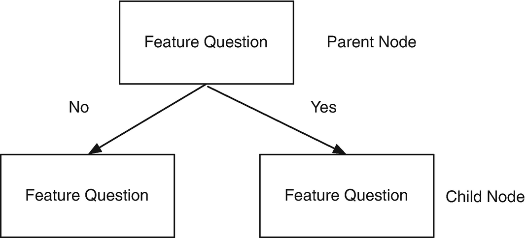
    ../images/420697_2_En_7_Chapter/420697_2_En_7_Fig4_HTML.png
    Figure 7.4

    Parent/child nodes.

  • What value of the parameter to use in the decision.

Training is done using the Gini values given in the previous recipe. We use the MATLAB-function fminbnd at each node, once for each of the two parameters. fminbnd is a one-dimensional local minimizer that finds the minimum of a function between two specified endpoints. If you know the range of interest, then this is a very effective way to find the minimum.
$$\displaystyle \begin{aligned} \underset{x} \min~f(x) \mbox{ such that}~ x_1 &lt; x &lt; x_2 \end{aligned} $$
(7.6)

There are two actions, “train” and “test.” “train” creates the decision tree and “test” runs the generated decision tree. You can also input your own decision tree. FindOptimalAction finds the parameter that minimizes the inhomogeneity on both sides of the division. The function called by fminbnd is RHSGT. We only implement the greater than action. The function call is:

function [d, r] = DecisionTree( action, d, t )  

action is a string that is either “train” or “test.” d is the data structure that defines the tree. t are the inputs for either training or testing. The outputs are the updated data structure and r with the results.

The function is first called with training data and the action is “train.” The main function is short.

 switch  lower (action)
   case  ’train’
     d = Training( d, t );
     d.box(1)
   case  ’test’
      for k = 1:length(d.box)
       d.box(k).id = [];
      end
     [r, d] = Testing( d, t );
      for k = 1:length(d.box)
       d.box(k)
      end
   otherwise
      error( ’%s is not an available action’,action);
end

We added the error case otherwise for completeness. Note that we use lower to eliminate case sensitivity. Training creates the decision tree. A decision tree is a set of boxes connected by lines. A parent box has two child boxes if it is a decision box. A class box has no children. The subfunction Training trains the tree. It adds boxes at each node.

  %% DecisionTree>Training
function d = Training( d, t )
 [n,m]   =  size (t.x);
 nClass  =  max (t.m);
 box(1) = AddBox( 1, 1:n*m, [] );
 box(1).child = [2 3];
 [~, dH] = HomogeneityMeasure(  ’initialize’, d, t.m );
 class   = 0;
 nRow    = 1;
 kR0     = 0;
 kNR0    = 1;  % Next row;
 kInRow  = 1;
 kInNRow = 1;
while( class < nClass )
   k   = kR0 + kInRow;
   idK   = box(k).id;  % Data that is in the box and to use to compute the next action
    % Enter this loop if it not a non-decision box
    ifisempty(box(k).class) )
     [action, param, val, cMin]  = FindOptimalAction( t, idK, d.xLim, d.yLim, dH );
     box(k).value                = val;
     box(k).param                = param;
     box(k).action               = action;
     x                           = t.x(idK);
     y                           = t.y(idK);
      if( box(k).param == 1 )  % x
       id  =  find (x >   d.box(k).value );
       idX =  find (x <=   d.box(k).value );
      else  % y
       id  =  find (y >  d.box(k).value );
       idX =  find (y <=   d.box(k).value );
      end
      % Child boxes
      if( cMin < d.cMin)  % Means we are in a class box
       class         = class + 1;
       kN            = kNR0 + kInNRow;
       box(k).child  = [kN kN+1];
       box(kN)       = AddBox( kN, idK(id), class  );
       class         = class + 1;
       kInNRow       = kInNRow + 1;
       kN            = kNR0 + kInNRow;
       box(kN)       = AddBox( kN, idK(idX), class );
       kInNRow       = kInNRow + 1;
      else
       kN            = kNR0 + kInNRow;
       box(k).child  = [kN kN+1];
       box(kN)       = AddBox( kN, idK(id)  );
       kInNRow       = kInNRow + 1;
       kN            = kNR0 + kInNRow;
       box(kN)       = AddBox( kN, idK(idX) );
       kInNRow       = kInNRow + 1;
      end
    end
          % Update current row
   kInRow   = kInRow + 1;
    if( kInRow > nRow )
     kR0       = kR0 + nRow;
     nRow      = 2*nRow;  % Add two rows
     kNR0      = kNR0 + nRow;
     kInRow    = 1;
     kInNRow   = 1;
    end
end
for k = 1:length(box)
    if( ~isempty(box(k).class) )
     box(k).child = [];
    end
   box(k).id = [];
    fprintf(1, ’Box %3d action %2s Value %4.1f\n’,k,box(k).action,box(k).value);
end
 d.box = box;  

We use fminbnd to find the optimal switch point. We need to compute the homogeneity on both sides of the switch and sum the values. The sum is minimized by fminbnd in the subfunction FindOptimalAction. This code is designed for rectangular region classes. Other boundaries won’t necessarily work correctly. The code is fairly involved. It needs to keep track of the box numbering to make the parent child connections. When the homogeneity measure is low enough, it marks the boxes as containing the classes.

The data structure box has multiple fields. One is the action to be taken in a decision box. The param is 1 for x and anything else for y. That determines if it is making the decision based on x or y. The value is the value used in the decision. child are indexes to the box children. The remaining code determines which row the box is in. class boxes have no children. The fields are shown in Table 7.1.
Table 7.1

Box Data Structure Fields

Field

Decision Box

Class Box

action

String

Not used

value

Value to be used in the decision

Not used

param

x or y

Not used

child

Array with two children

Empty

id

Empty

ID of data in the class

class

Class ID

Not used

7.5 Creating a Handmade Tree

7.5.1 Problem

We want to test a handmade decision tree.

7.5.2 Solution

The solution is to write a script to test a handmade decision tree.

7.5.3 How It Works

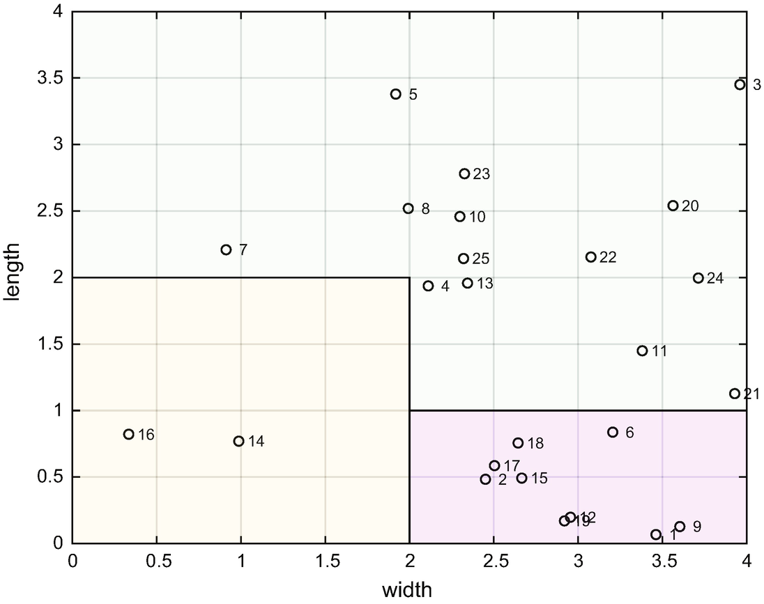
We write the test script SimpleClassifierDemo shown below. It uses the ’test’ action for DecisionTree. It generates 52 points. We create rectangular regions so that the face arrays have four elements for each polygon. DrawBinaryTree draws the tree.

 d = DecisionTree;
  % Vertices for the sets
 v = [ 0 0; 0 4; 4 4; 4 0; 2 4; 2 2; 2 0; 0 2; 4 2];
  % Faces for the sets
 f = { [6 5 2 8] [6 7 4 9] [6 9 3 5] [1 7 6 8] };
  % Generate the testing set
 pTest  = ClassifierSets( 5, [0 4], [0 4], { ’width’,  ’length’}, v, f,  ’Testing Set’ );
  % Test the tree
 [d, r] = DecisionTree(  ’test’,  d, pTest  );
 q = DrawBinaryTree;
 c =  ’xy’;
for k = 1:length(d.box)
    if( ~isempty(d.box(k).action) )
     q.box{k} =  sprintf ( ’%c %s %4.1f’,c(d.box(k).param),d.box(k).action,d.box(k).value);
    else
     q.box{k} =  sprintf ( ’Class %d’,d.box(k).class);
    end
end
 DrawBinaryTree(q);
 m =  reshape (pTest.m,[],1);
for k = 1:length(r)
    fprintf(1, ’Class %d\n’,m(r{k}(1)));
    for j = 1:length(r{k})
      fprintf(1, ’%d ’,r{k}(j));
    end
    fprintf(1, ’\n’)
end

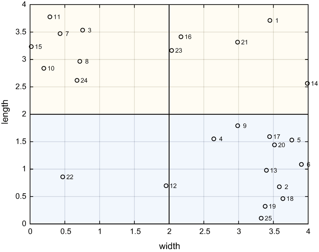
SimpleClassifierDemo uses the hand-built example in DecisionTree.

function d = DefaultDataStructure
  %% DecisionTree>DefaultDataStructure
  % Generate a default data structure
 d.tree          = DrawBinaryTree;
 d.threshold     = 0.01;
 d.xLim          = [0 4];
 d.yLim          = [0 4];
 d.data      = [];
 d.cMin          = 0.01;
 d.box(1)    = struct( ’action’, ’>’, ’value’,2, ’param’,1, ’child’,[2 3], ’id’,[], ’class’,[]);
 d.box(2)    = struct( ’action’, ’>’, ’value’,2, ’param’,2, ’child’,[4 5], ’id’,[], ’class’,[]);
 d.box(3)    = struct( ’action’, ’>’, ’value’,2, ’param’,2, ’child’,[6 7], ’id’,[], ’class’,[]);
for k = 4:7
   d.box(k) = struct( ’action’, ’’, ’value’,0, ’param’,0, ’child’,[], ’id’,[], ’class’,[]);
end
Figure 7.5 shows the results from SimpleClassifierDemo. There are four rectangular areas, which are our sets.
../images/420697_2_En_7_Chapter/420697_2_En_7_Fig5_HTML.png
Figure 7.5

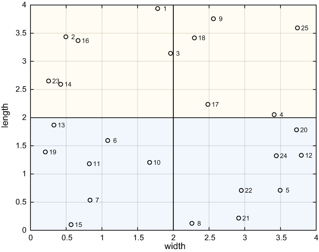
Data and classes in the test set.

We can create a decision tree by hand as shown Figure 7.6.
../images/420697_2_En_7_Chapter/420697_2_En_7_Fig6_HTML.png
Figure 7.6

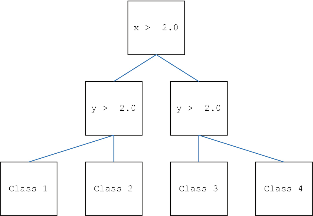
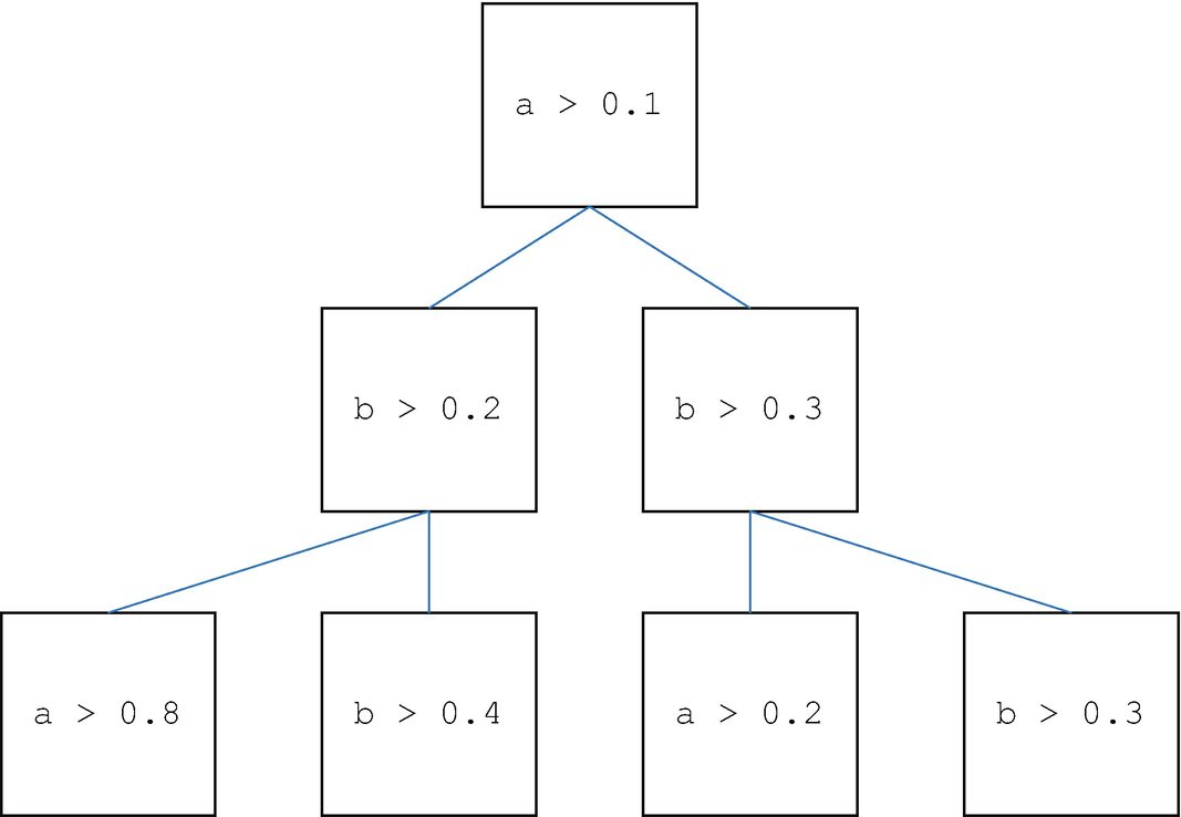
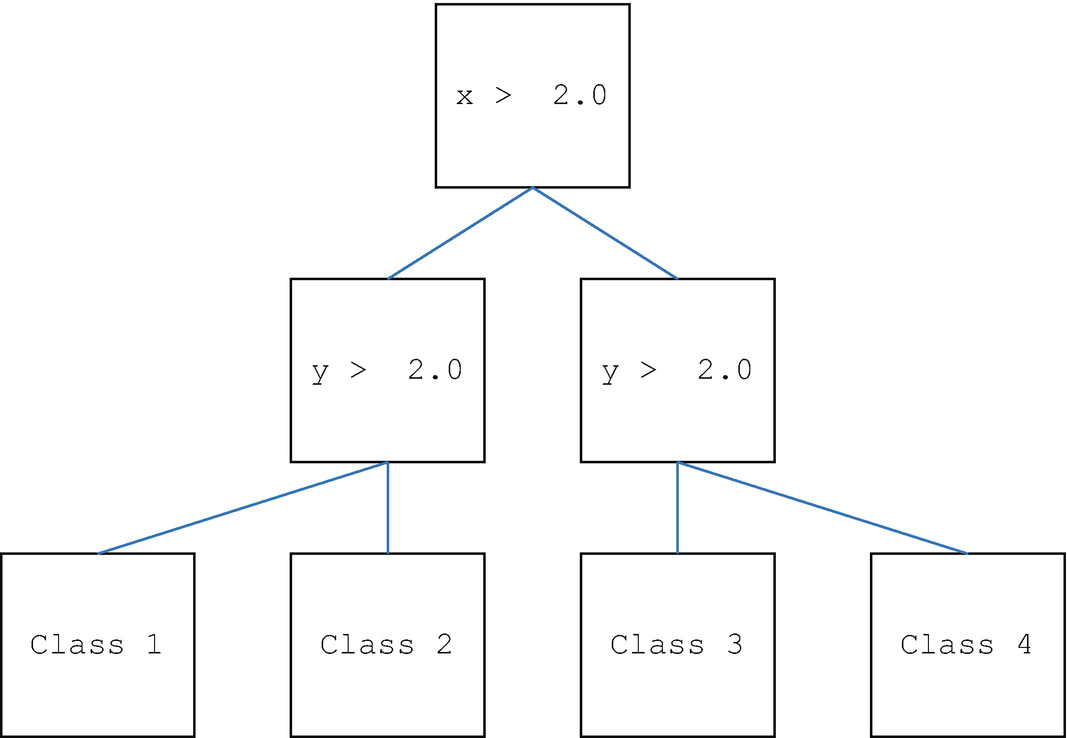
A manually created decision tree. The drawing is generated by DecisionTree. The last row of boxes is the data sorted into the four classes. The last nodes are the classes. Each box is a decision tree node.

The decision tree sorts the samples into the four sets. In this case, we know the boundaries and can use them to write the inequalities. In software, we will have to determine what values provide the shortest branches. The following is the output of SimpleClassifierDemo. The decision tree properly classifies all of the data.

 >> SimpleClassifierDemo
 Class 3
 4 6 9 13 18
 Class 2
 7 14 17 21
 Class 1
 1 2 5 8 10 11 12 23 25
 Class 4
 3 15 16 19 20 22 24  

7.6 Training and Testing

7.6.1 Problem

We want to train our decision tree and test the results.

7.6.2 Solution

We replicated the previous recipe, only this time we have DecisionTree create the decision tree instead of creating it by hand.

7.6.3 How It Works

TestDecisionTree trains and tests the decision tree. It is very similar to the code for the hand-built decision tree demo, SimpleClassifierDemo. Once again, we use rectangles for the regions.

  % Vertices for the sets
 v = [ 0 0; 0 4; 4 4; 4 0; 2 4; 2 2; 2 0; 0 2; 4 2];
  % Faces for the sets
 f = { [6 5 2 8] [6 7 4 9] [6 9 3 5] [1 7 6 8] };
  % Generate the training set
 pTrain = ClassifierSets( 40, [0 4], [0 4], { ’width’,  ’length’},...
   v, f,  ’Training Set’ );
  % Create the decision tree
 d      = DecisionTree;
 d      = DecisionTree(  ’train’, d, pTrain );
  % Generate the testing set
 pTest  = ClassifierSets( 5, [0 4], [0 4], { ’width’,  ’length’},...
   v, f,  ’Testing Set’ );
  % Test the tree
 [d, r] = DecisionTree(  ’test’,  d, pTest  );
 q = DrawBinaryTree;
 c =  ’xy’;
for k = 1:length(d.box)
    if( ~isempty(d.box(k).action) )
     q.box{k} =  sprintf ( ’%c %s %4.1f’,c(d.box(k).param),...
       d.box(k).action,d.box(k).value);
    else
     q.box{k} =  sprintf ( ’Class %d’,d.box(k).class);
    end
end
 DrawBinaryTree(q);
 m =  reshape (pTest.m,[],1);
for k = 1:length(r)
    fprintf(1, ’Class %d\n’,m(r{k}(1)));
    for j = 1:length(r{k})
      fprintf(1, ’%d ’,r{k}(j));
    end

It uses ClassifierSets to generate the training data. The output includes the coordinates and the sets in which they fall. We then create the default data structure and call DecisionTree in training mode.

The tree is shown in Figure 7.9. The training data are shown in Figure 7.7 and the testing data in Figure 7.8. We need enough testing data to fill the classes. Otherwise, the decision tree generator may draw the lines to encompass just the data in the training set.
../images/420697_2_En_7_Chapter/420697_2_En_7_Fig7_HTML.jpg
Figure 7.7

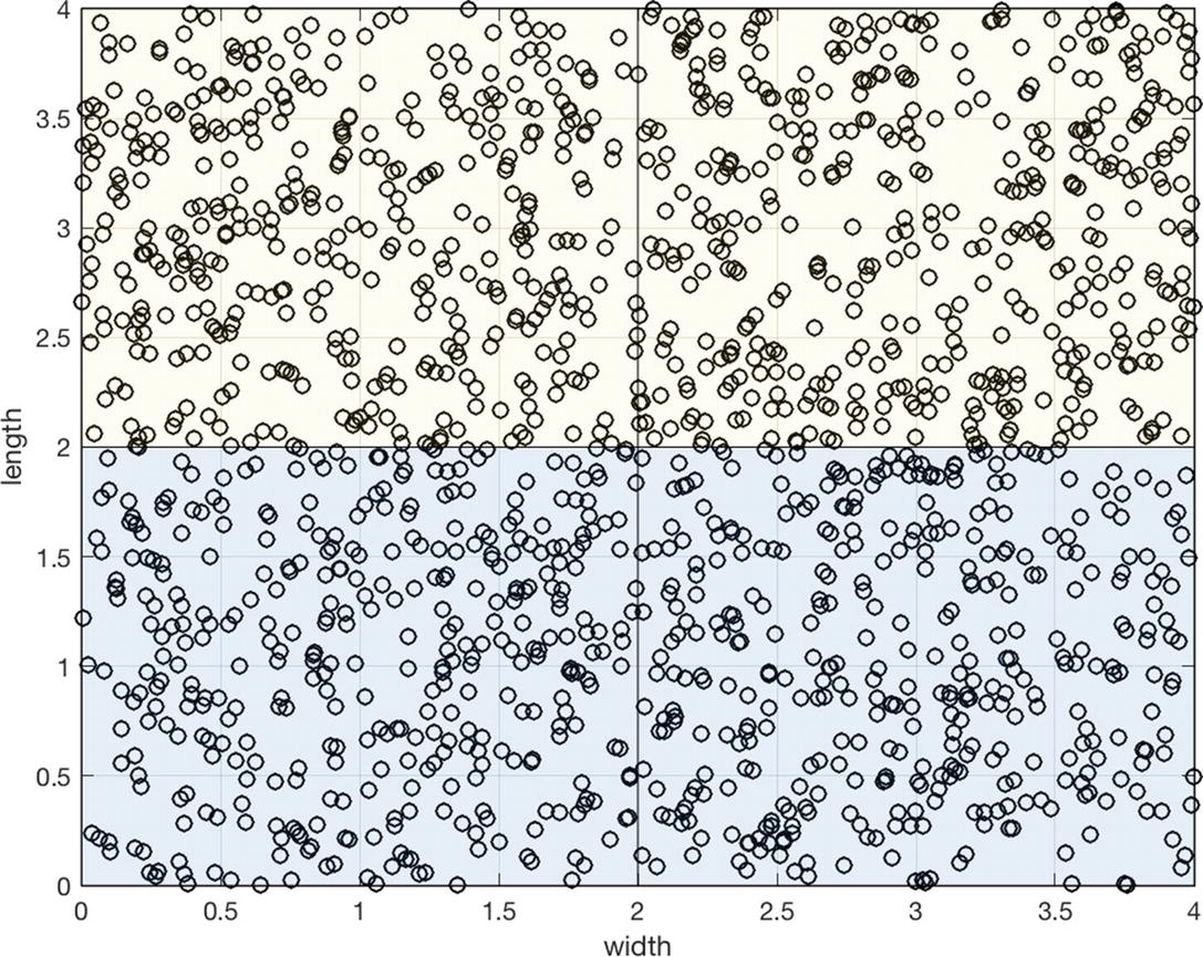
The training data. A large amount of data is needed to fill the classes.

../images/420697_2_En_7_Chapter/420697_2_En_7_Fig8_HTML.png
Figure 7.8

The testing data.

../images/420697_2_En_7_Chapter/420697_2_En_7_Fig9_HTML.png
Figure 7.9

The tree derived from the training data. It is essentially the same as the hand-derived tree. The values in the generated tree are not exactly 2.0.

The results are similar to the simple test.

 Class 3
 1 14 16 21 23
 Class 2
 2 4 5 6 9 13 17 18 19 20 25
 Class 1
 3 7 8 10 11 15 24
 Class 4
 12 22  

The generated tree separates the data effectively.

7.7 Summary

This chapter has demonstrated data classification using decision trees in MATLAB. We also wrote a new graphics function to draw decision trees. The decision tree software is not general purpose, but can serve as a guide to more general purpose code. Table 7.2 lists the functions and scripts included in the companion code.
Table 7.2

Chapter Code Listing

File

Description

ClassifierSets

Generate data for classification or training.

DecisionTree

Implements a decision tree to classify data.

DrawBinaryTree

Generates data for classification or training.

HomogeneityMeasure

Computes Gini impurity.

SimpleClassifierDemo

Demonstrates decision tree testing.

SimpleClassifierExample

Generates data for a simple problem.

TestDecisionTree

Tests a decision tree.