2.1 Introduction to MATLAB Data Types
2.1.1 Matrices
By default, all variables in MATLAB are double precision matrices. You do not need to declare a type for these variables. Matrices can be multidimensional and are accessed using 1-based indices via parentheses. You can address elements of a matrix using a single index, taken column-wise, or one index per dimension. To create a matrix variable, simply assign a value to it, such as this 2x2 matrix a:
TIP
A semicolon terminates an expression so that it does not appear in the command window. If you leave out the semicolon, it will print in the command window. Leaving out semicolons is a convenient way of debugging without using the MATLAB debugger, but it can be hard to find those missing semicolons later!
You can simply add, subtract, multiply, and divide matrices with no special syntax. The matrices must be the correct size for the linear algebra operation requested. A transpose is indicated using a single quote suffix, A’, and the matrix power uses the operator ̂.
By default, every variable is a numerical variable. You can initialize matrices to a given size using the zeros, ones, eye, or rand functions, which produce zeros, ones, identity matrices (ones on the diagonal), and random numbers respectively. Use isnumeric to identify numeric variables.
Key Functions for Matrices
Function | Purpose |
|---|---|
zeros | Initialize a matrix to zeros |
ones | Initialize a matrix to ones |
eye | Initialize an identity matrix |
rand, randn | Initialize a matrix of random numbers |
isnumeric | Identify a matrix or scalar numeric value |
isscalar | Identify a scalar value (a 1 x 1 matrix) |
size | Return the size of the matrix |
MATLAB can support n-dimensional arrays. A two-dimensional array is like a table. A three-dimensional array can be visualized as a cube where each box inside the cube contains a number. A four-dimensional array is harder to visualize, but we needn’t stop there!
2.1.2 Cell Arrays
One variable type unique to MATLAB is cell arrays. This is really a list container, and you can store variables of any type in elements of a cell array. Cell arrays can be multi-dimensional, just like matrices, and are useful in many contexts.
Cell arrays are indicated by curly braces, {}. They can be of any dimension and contain any data, including string, structures, and objects. You can initialize them using the cell function, recursively display the contents using celldisp, and access subsets using parentheses, just like for a matrix. A short example is below.
Using curly braces for access gives you the element data as the underlying type. When you access elements of a cell array using parentheses, the contents are returned as another cell array, rather than the cell contents. MATLAB help has a special section called Comma-Separated Lists, which highlights the use of cell arrays as lists. The code analyzer will also suggest more efficient ways to use cell arrays. For instance,
Replace
a = {b{:} c};
with
a = [b {c}];
Cell arrays are especially useful for sets of strings, with many of MATLAB’s string search functions optimized for cell arrays, such as strcmp.
Use iscell to identify cell array variables. Use deal to manipulate structure array and cell array contents.
Key Functions for Cell Arrays
Function | Purpose |
|---|---|
cell | Initialize a cell array |
cellstr | Create a cell array from a character array |
iscell | Identify a cell array |
iscellstr | Identify a cell array containing only strings |
celldisp | Recursively display the contents of a cell array |
2.1.3 Data Structures
Data structures in MATLAB are highly flexible, leaving it up to the user to enforce consistency in fields and types. You are not required to initialize a data structure before assigning fields to it, but it is a good idea to do so, especially in scripts, to avoid variable conflicts.
Replace
d.fieldName = 0;
with
In fact, we have found it generally a good idea to create a special function to initialize larger structures that are used throughout a set of functions. This is similar to creating a class definition. Generating your data structure from a function, instead of typing out the fields in a script, means that you always start with the correct fields. Having an initialization function also allows you to specify the types of variables and provide sample or default data. Remember, since MATLAB does not require you to declare variable types, doing so yourself with default data makes your code that much clearer.
TIP
Create an initialization function for data structures.
You make a data structure into an array simply by assigning an additional copy. The fields must be identically named (they are case-sensitive) and in the same order, which is yet another reason to use a function to initialize your structure. You can nest data structures with no limit on depth.
MATLAB now allows for dynamic field names using variables, i.e., structName.( dynamicExpression). This provides improved performance over getfield, where the field name is passed as a string. This allows for all sorts of inventive structure programming. Take our data structure array in the previous code snippet, and let’s get the values of field a using a dynamic field name; the values are returned in a cell array.
Use isstruct to identify structure variables and isfield to check for the existence of fields. Note that isempty will return false for a struct initialized with struct, even if it has no fields.
Key Functions for Structs
Function | Purpose |
|---|---|
struct | Initialize a structure with or without fields |
isstruct | Identify a structure |
isfield | Determine if a field exists in a structure |
fieldnames | Get the fields of a structure in a cell array |
rmfield | Remove a field from a structure |
deal | Set fields in a structure array to a value |
2.1.4 Numerics
Although MATLAB defaults to doubles for any data entered at the command line or in a script, you can specify a variety of other numeric types, including single, uint8, uint16, uint32, uint64, logical (i.e., an array of Booleans). Use of the integer types is especially relevant to using large data sets such as images. Use the minimum data type you need, especially when your data sets are large.
2.1.5 Images
MATLAB supports a variety of formats including GIF, JPG, TIFF, PNG, HDF, FITS, and BMP. You can read in an image directly using imread, which can determine the type automatically from the extension, or fitsread. (FITS stands for Flexible Image Transport System and the interface is provided by the CFITSIO library.) imread has special syntaxes for some image types, such as handling alpha channels for PNG, so you should review the options for your specific images. imformats manages the file format registry and allows you to specify handling of new user-defined types, if you can provide read and write functions.
You can display an image using either imshow, image, or imagesc, which scales the colormap for the range of data in the image.
For example, we use a set of images of cats in Chapter 7, on face recognition. The following is the image information for one of these sample images
These are the metadata that tell camera software, and image databases, where and how the image was generated. This is useful when learning from images as it allows you to correct for resolution (width and height) bit depth and other factors.
If we view this image using imshow, it will publish a warning that the image is too big to fit on the screen and that it is displayed at 33%. If we view it using image, there will be a visible set of axes. image is useful for displaying other two-dimensional matrix data such as individual elements per pixel. Both functions return a handle to an image object; only the axes’ properties are different.
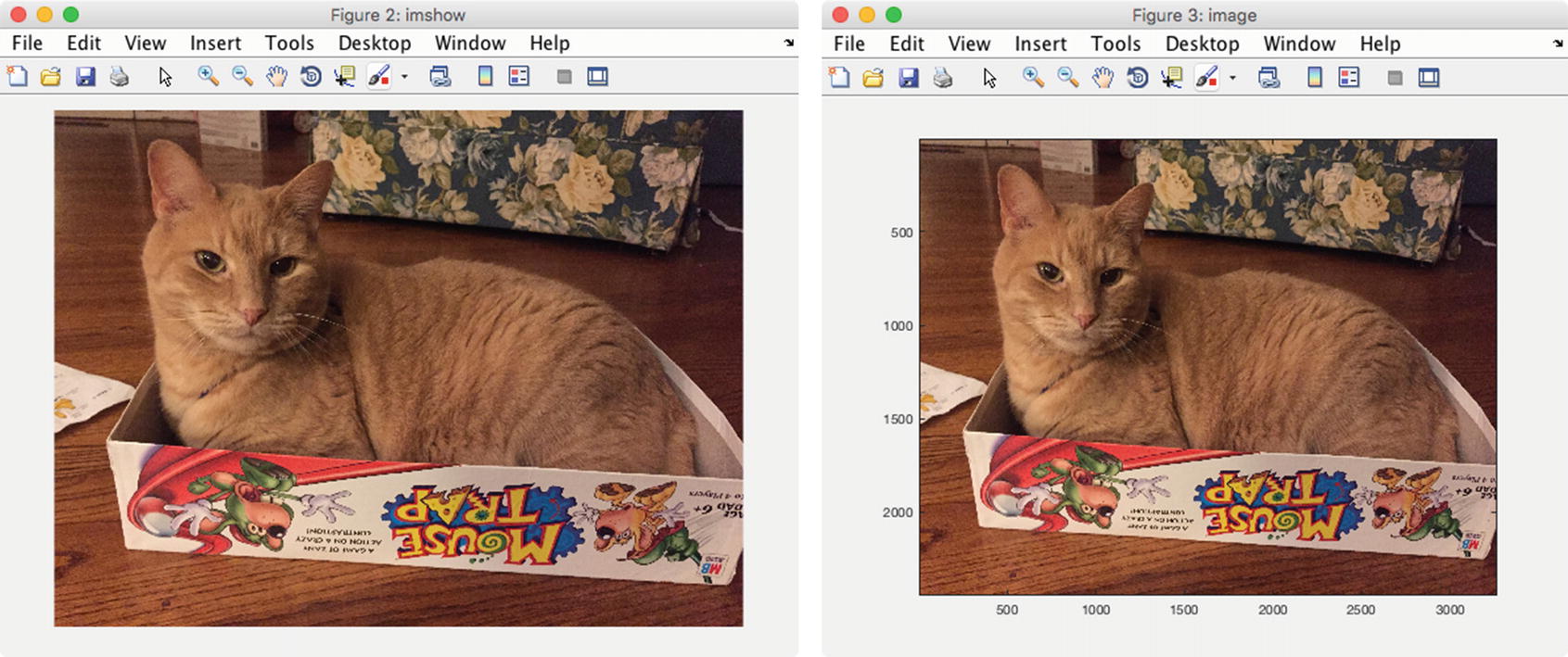
Image display options.
Key Functions for Images
Function | Purpose |
|---|---|
imread | Read an image in a variety of formats |
imfinfo | Gather information about an image file |
imformats | Determine if a field exists in a structure |
imwrite | Write data to an image file |
image | Display image from array |
imagesc | Display image data scaled to the current colormap |
imshow | Display an image, optimizing figure, axes, and image object properties, and taking an array or a filename as an input |
rgb2gray | Write data to an image file |
ind2rgb | Convert index data to RGB |
rgb2ind | Convert RGB data to indexed image data |
fitsread | Read a FITS file |
fitswrite | Write data to a FITS file |
fitsinfo | Information about a FITS file returned in a data structure |
fitsdisp | Display FITS file metadata for all HDUs in the file |
2.1.6 Datastore
Datastores allow you to interact with files containing data that are too large to fit in memory. There are different types of datastores for tabular data, images, spreadsheets, databases, and custom files. Each datastore provides functions to extract smaller amounts of data that fit in the memory for analysis. For example, you can search a collection of images for those with the brightest pixels or maximum saturation values. We will use our directory of cat images as an example.
Once the datastore is created, you use the applicable class functions to interact with it. Datastores have standard container-style functions such as read, partition, and reset. Each type of datastore has different properties. The DatabaseDatastore requires the Database Toolbox, and allows you to use SQL queries.
MATLAB provides the MapReduce framework for working with out-of-memory data in datastores. The input data can be any of the datastore types, and the output is a key-value datastore. The map function processes the datastore input in chunks and the reduce function calculates the output values for each key. mapreduce can be sped up by using it with the MATLAB Parallel Computing Toolbox, Distributed Computer Server, or Compiler.
Key Functions for Datastore
Function | Purpose |
|---|---|
datastore | Create a datastore |
read | Read a subset of data from the datastore |
readall | Read all of the data in the datastore |
hasdata | Check to see if there are more data in the datastore |
reset | Initialize a datastore with the contents of a folder |
partition | Excerpt a portion of the datastore |
numpartitions | Estimate a reasonable number of partitions |
ImageDatastore | Datastore of a list of image files. |
TabularTextDatastore | A collection of one or more tabular text files. |
SpreadsheetDatastore | Datastore of spreadsheets. |
FileDatastore | Datastore for files with a custom format, for which you provide a reader function. |
KeyValueDatastore | Datastore of key-value pairs. |
DatabaseDatastore | Database connection, requires the Database Toolbox. |
2.1.7 Tall Arrays
Tall arrays were introduced in R2016b Release of MATLAB. They are allowed to have more rows than will fit in the memory. You can use them to work with datastores that might have millions of rows. Tall arrays can use almost any MATLAB type as a column variable, including numeric data, cell arrays, strings, datetimes, and categoricals. The MATLAB documentation provides a list of functions that support tall arrays. Results for operations on the array are only evaluated when they are explicitly requested using the gather function. The histogram function can be used with tall arrays and will execute immediately.
Tall Arrays
Analysis of Big Data with Tall Arrays
Functions That Support Tall Arrays (A–Z)
Index and View Tall Array Elements
Visualization of Tall Arrays
Extend Tall Arrays with Other Products
Tall Array Support, Usage Notes, and Limitations
Key Functions for Tall Arrays
Function | Purpose |
|---|---|
tall | Initialize a tall array |
gather | Execute the requested operations |
summary | Display summary information to the command line |
head | Access the first rows of a tall array |
tail | Access the last rows of a tall array |
istall | Check the type of array to determine if it is tall |
write | Write the tall array to disk |
2.1.8 Sparse Matrices
Sparse matrices are a special category of matrix in which most of the elements are zero. They appear commonly in large optimization problems and are used by many such packages. The zeros are “squeezed” out and MATLAB stores only the nonzero elements along with index data such that the full matrix can be recreated. Many regular MATLAB functions, such as chol or diag, preserve the sparseness of an input matrix.
2.1.9 Tables and Categoricals
Key Functions for Sparse Matrices
Function | Purpose |
|---|---|
sparse | Create a sparse matrix from a full matrix or from a list of indices and values |
issparse | Determine if a matrix is sparse |
nnz | Number of nonzero elements in a sparse matrix |
spalloc | Allocate a nonzero space for a sparse matrix |
spy | Visualize a sparsity pattern |
spfun | Selectively apply a function to the nonzero elements of a sparse matrix |
full | Convert a sparse matrix to full form |
Categorical arrays allow for storage of discrete non-numeric data, and they are often used within a table to define groups of rows. For example, time data may have the day of the week, or geographic data may be organized by state or county. They can be leveraged to rearrange data in a table using unstack.
You can also combine multiple data sets into single tables using join, innerjoin, and outerjoin, which will be familiar to you if you have worked with databases.
Key Functions for Tables
Function | Purpose |
|---|---|
table | Create a table with data in the workspace |
readtable | Create a table from a file |
join | Merge tables by matching up variables |
innerjoin | Join tables A and B retaining only the rows that match |
outerjoin | Join tables including all rows |
stack | Stack data from multiple table variables into one variable |
unstack | Unstack data from a single variable into multiple variables |
summary | Calculate and display summary data for the table |
categorical | Arrays of discrete categorical data |
iscategorical | Create a categorical array |
categories | List of categories in the array |
iscategory | Test for a particular category |
addcats | Add categories to an array |
removecats | Remove categories from an array |
mergecats | Merge categories |
2.1.10 Large MAT-Files
You can access parts of a large MAT-file without loading the entire file into the memory by using the matfile function. This creates an object that is connected to the requested MAT-file without loading it. Data are only loaded when you request a particular variable, or part of a variable. You can also dynamically add new data to the MAT-file.
For example, we can load a MAT-file of neural net weights generated in a later chapter.
We can access a portion of the previously unloaded w variable, or add a new variable name, all using this object m.
There are some limits to the indexing into unloaded data, such as struct arrays and sparse arrays. Also, matfile requires MAT-files using version 7.3, which is not the default for a generic save operation as of R2016b Release of MATLAB. You must either create the MAT-file using matfile to take advantage of these features or use the -v7.3’ flag when saving the file.
2.2 Initializing a Data Structure Using Parameters
It’s always a good idea to use a special function to define a data structure you are using as a type in your codebase, similar to writing a class but with less overhead. Users can then overload individual fields in their code, but there is an alternative way of setting many fields at once: an initialization function that can handle a parameter pair input list. This allows you to do additional processing in your initialization function. Also, your parameter string names can be more descriptive than you would choose to make your field names.
2.2.1 Problem
We want to initialize a data structure so that the user clearly knows what he or she is entering.
2.2.2 Solution
The simplest way of implementing the parameter pairs is using varargin and a switch statement. Alternatively, you could write an inputParser, which allows you to specify required and optional inputs as well as named parameters. In that case, you have to write separate or anonymous functions for validation that can be passed to the inputParser, rather than just write out the validation in your code.
2.2.3 How It Works
We will use the data structure developed for the automobile simulation in Chapter 12 as an example. The header lists the input parameters along with the input dimensions and units, if applicable.
The function first creates the data structure using a set of defaults, then handles the parameter pairs entered by a user. After the parameters have been processed, two areas are calculated using the dimensions and the height.
To perform the same tasks with inputParser, you add a addRequired, addOptional, or addParameter call for every item in the switch statement. The named parameters require default values. You can optionally specify a validation function; in the example below we use isNumeric to limit the values to numeric data.
In this case, the results of the parsed parameters are stored in a Results substructure.
2.3 Performing MapReduce on an Image Datastore
2.3.1 Problem
We discussed the datastore class in the introduction to the chapter. Now let’s use it to perform analysis on the full set of cat images using mapreduce, which is scalable to very large numbers of images. This involves two steps; first a map step that operates on the datastore and creates intermediate values, and then a reduce step that operates on the intermediate values to produce a final output.
2.3.2 Solution
We create the datastore by passing in the path to the folder of cat images. We also need to create a map function and a reduce function, to pass into mapreduce. If you are using additional toolboxes such as the Parallel Computing Toolbox, you would specify the reduce environment using mapreducer.
2.3.3 How It Works
First, create the datastore using the path to the images.
Second, we write the map function. This must generate and store a set of intermediate values that will be processed by the reduce function. Each intermediate value must be stored as a key in the intermediate key-value datastore using add. In this case, the map function will receive one image each time it is called. We call it catColorMapper, since it processes the red, green, and blue values for each image using a simple average.
The reduce function will then receive the list of image files from the datastore once for each key in the intermediate data. It receives an iterator to the intermediate data store as well as an output data store. Again, each output must be a key-value pair. The hasnext and getnext functions used are part of the mapreduce ValueIterator class. In this case, we find the minimum value for each key across the set of images.
Finally, we call mapreduce using function handles to our two helper functions. Progress updates are printed to the command line, first for the mapping step, and then for the reduce step (once the mapping progress reaches 100%).
The results are stored in a MAT-file, for example, results_1_28-Sep-2016_16-28- 38_347. The store returned is a key-value store to this MAT-file, which in turn contains the store with the final key-value results.
You’ll notice that the image files are different file types. This is because they came from different sources. MATLAB can handle most image types quite well.
2.4 Creating a Table from a File
Often with big data we have complex data in many files. MATLAB provides functions to make it easier to handle massive sets of data. In this section, we will collect data from a set of weather files and perform a Fast Fourier Transform (FFT) on data from two years. First, we will write the FFT function.
2.4.1 Problem
We want do FFTs.
2.4.2 Solution
Write a function using fft and compute the energy from the FFT. The energy is just the real part of the product of the FFT output and its transpose.
2.4.3 How It Works
The following functions takes in data y with a sample time tSamp and performs an FFT
We get the energy using these two lines
Taking the real part just accounts for numerical errors. The product of a number and its complex conjugate should be real.
The function computes the resolution. Notice it is a function of the sampling period and number of points.
The built-in demo creates a series with a frequency at 1 rad/sec and a second at 2 rad/sec. The higher frequency one, with an amplitude of 2, has more energy as expected.
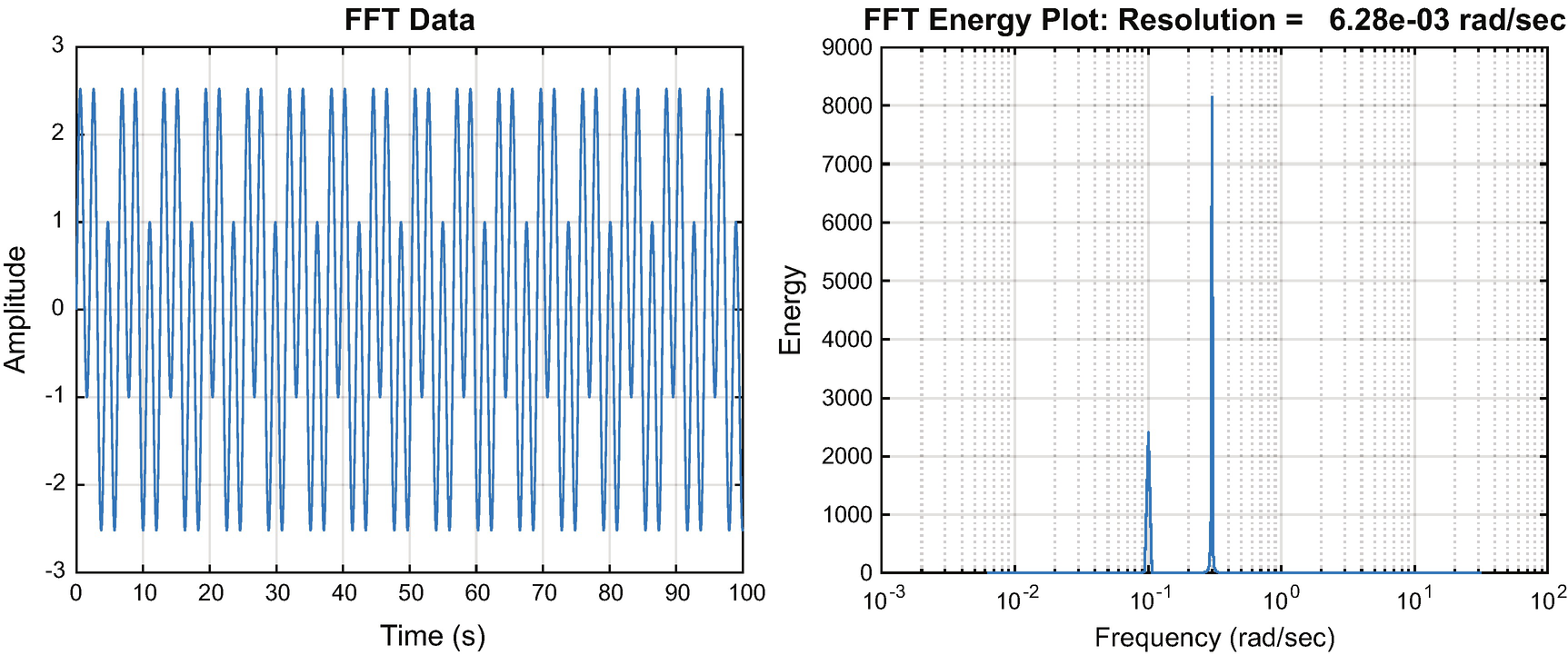
The input data for the FFT and the results.
2.5 Processing Table Data
2.5.1 Problem
We want to compare temperature frequencies in 1999 and 2015 using data from a table.
2.5.2 Solution
Use tabularTextDatastore to load the data and perform an FFT on the data.
2.5.3 How It Works
First, let us look at what happens when we read in the data from the weather files.
WeatherFFT selects the data to use. It finds all the data in the mess of data in the files. When running the script you need to be in the same folder as WeatherFFT.
If the data do not exist TabularTextDatastore puts NaN in the data points’ place. We happened to pick two years without any missing data. We use preview to see what we are getting.
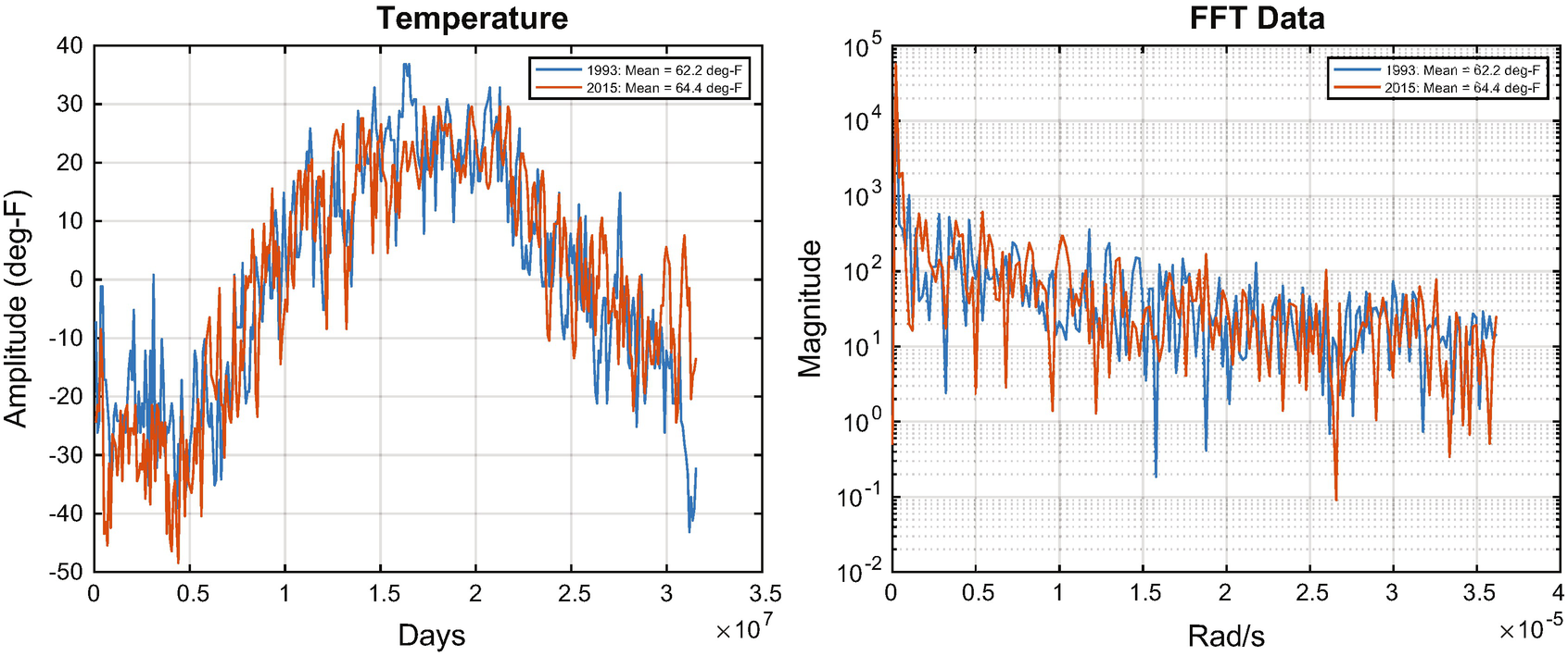
1993 and 2015 data.
We get a little fancy with plotset. Our legend entries are computed to include the mean temperatures.
2.6 Using MATLAB Strings
Machine learning often requires interaction with humans, which often means processing speech. Also, expert systems and fuzzy logic systems can make use of textual descriptions. MATLAB’s string data type makes this easier. Strings are bracketed by double quotes. In this section, we will give examples of operations that work with strings, but not with character arrays.
2.6.1 String Concatenation
2.6.1.1 Problem
We want to concatenate two strings.
2.6.1.2 Solution
Create the two strings and use the “+” operator.
2.6.1.3 How It Works
You can use the + operator to concatenate strings. The result is the second string after the first.
2.6.2 Arrays of Strings
2.6.2.1 Problem
We want any array of strings.
2.6.2.2 Solution
Create the two strings and put them in a matrix.
2.6.2.3 How It Works
We create the same two strings as above and use the matrix operator. If they were character arrays we would need to pad the shorter with blanks to be the same size as the longer.
You could have used a cell array for this, but strings are often more convenient.
2.6.3 Substrings
2.6.3.1 Problem
We want to get strings after a fixed prefix.
2.6.3.2 Solution
Create a string array and use extractAfter.
2.6.3.3 How It Works
Create a string array of strings to search and use extractAfter.
Most of the string functions work with char, but strings are a little cleaner. Here is the above example with cell arrays.
2.7 Summary
Chapter Code Listing
File | Description |
|---|---|
AutomobileInitialize | Data structure initialization example from Chapter 12. |
catReducer | Image datastore used with mapreduce. |
FFTEnergy | Computes the energy from an FFT. |
weatherFFT | Does an FFT of weather data. |