
Typically control systems are designed and implemented with all of the parameters hard coded into the software. This works very well in most circumstances, particularly when the system is well known during the design process. When the system is not well defined, or is expected to change significantly during operation, it may be necessary to implement learning control. For example, the batteries in an electric car degrade over time. This leads to less range. An autonomous driving system would need to learn that that range was decreasing. This would be done by comparing the distance traveled with the battery state of charge. More drastic, and sudden, changes can alter a system. For example, in an aircraft the air data system may fail owing to a sensor malfunction. If GPS were still operating, the plane would want to switch to a GPS-only system. In a multi-input-multi-output control system a branch may fail, because of a failed actuator or sensor. The system may have to modify to operating branches in that case.
Learning and adaptive control are often used interchangeably. In this chapter, you will learn a variety of techniques for adaptive control for different systems. Each technique is applied to a different system, but all are generally applicable to any control system.
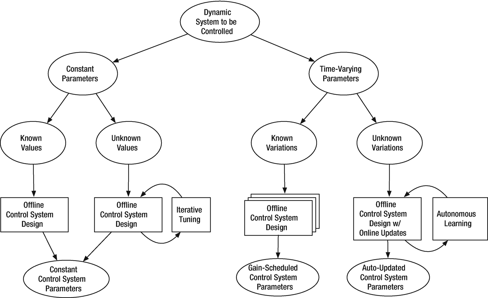
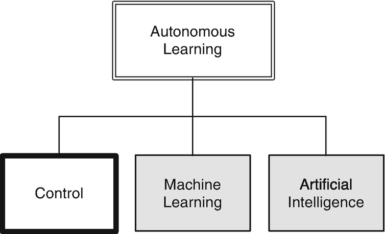
Taxonomy of adaptive or learning control.
The next example is for ship control. Your goal is to control the heading angle. The dynamics of the ship are a function of the forward speed. Although it isn’t really learning from experience, it is adapting based on information about its environment.
The last example is a spacecraft with variable inertia. This shows very simple parameter estimation.
5.1 Self Tuning: Modeling an Oscillator
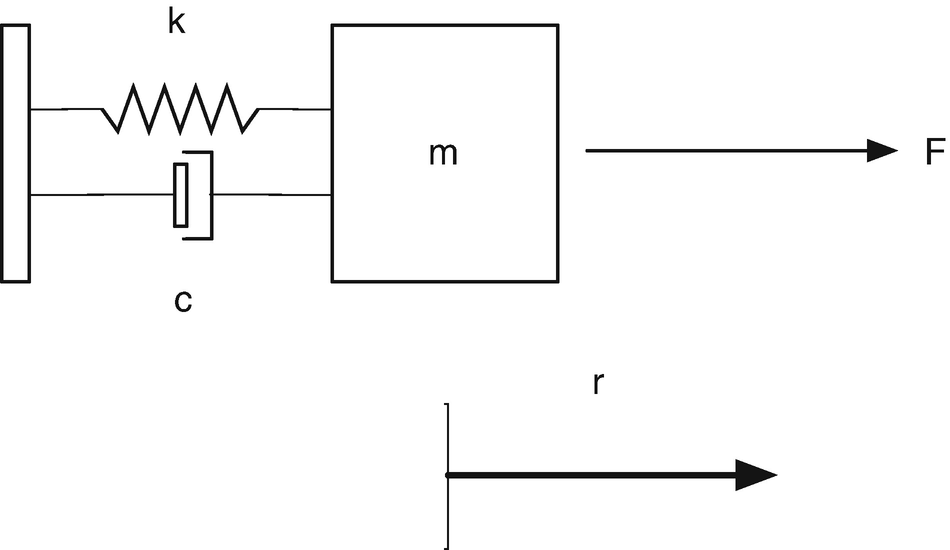
Spring-mass-damper system. The mass is on the right. The spring is on the top to the left of the mass. The damper is below. F is the external force, m is the mass, k is the stiffness, and c is the damping.


TIP
Weight is mass times the acceleration of gravity.


5.2 Self Tuning: Tuning an Oscillator
5.2.1 Problem
We want to identify the frequency of an oscillator and tune a control system to that frequency.
5.2.2 Solution
The solution is to have the control system measure the frequency of the spring. We will use an FFT to identify the frequency of the oscillation.
5.2.3 How It Works
The following script shows how an FFT identifies the oscillation frequency for a damped oscillator.


The following shows the simulation loop and FFTEnergy call.
FFTEnergy is shown below.
The FFT takes the sampled time sequence and computes the frequency spectrum. We compute the FFT using MATLAB’s fft function. We take the result and multiply it by its conjugate to get the energy. The first half of the result has the frequency information. aPeak is to indicate peaks for the output. It is just looking for values greater than a certain threshold.
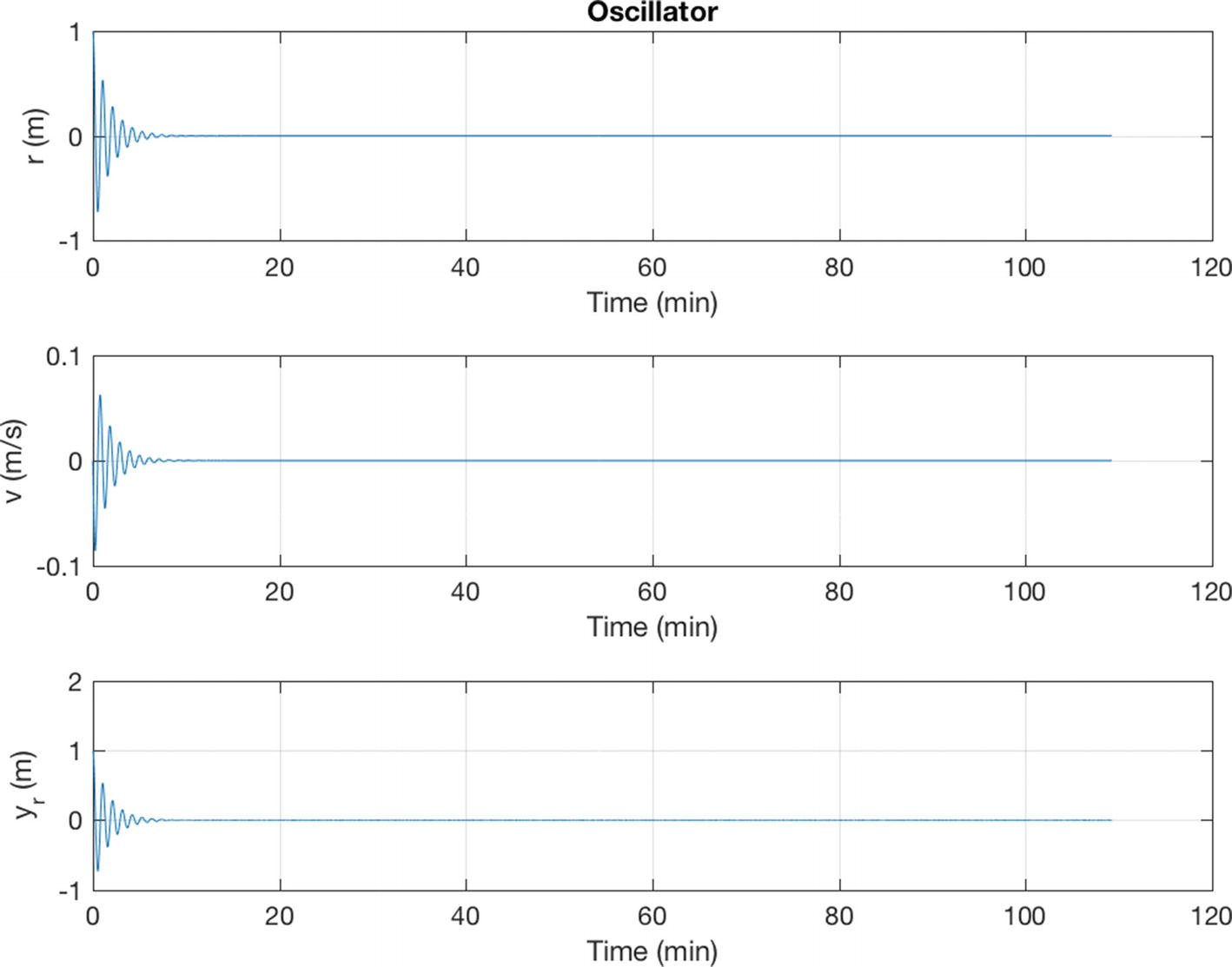
Simulation of the damped oscillator. The damping ratio, ζ is 0.5 and undamped natural frequency ω is 0.1 rad/s.
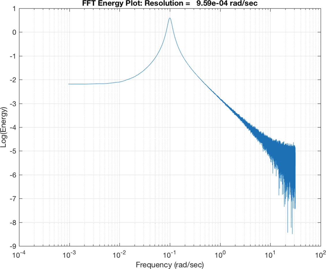
The frequency spectrum. The peak is at the oscillation frequency of 0.1 rad/s.
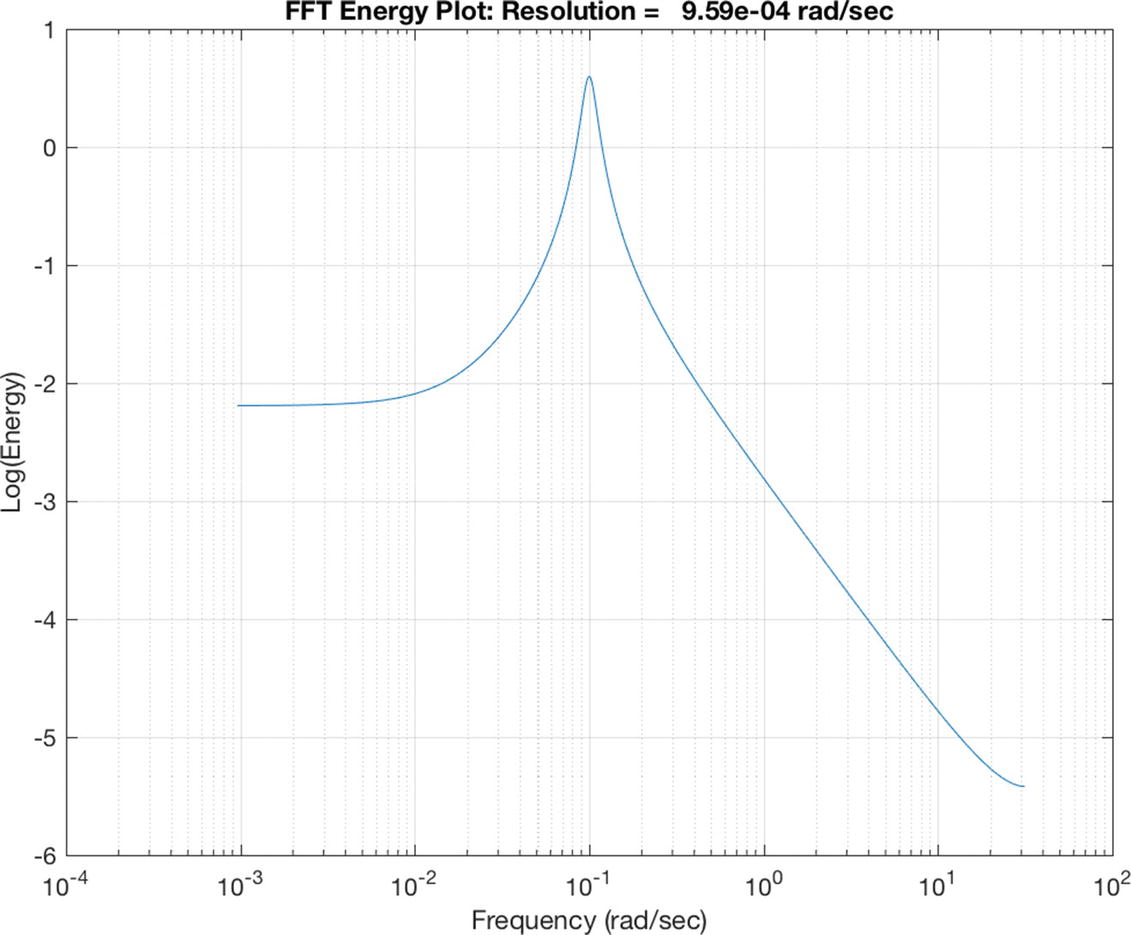
The frequency spectrum without noise. The peak of the spectrum is at 0.1 rad/s in agreement with the simulation.
- 1.
Excite the oscillator with a pulse
- 2.
Run it for 2n steps
- 3.
Do an FFT
- 4.
If there is only one peak, compute the damping gain
The script TuningSim calls FFTEnergy.m with aPeak set to 0.7. The value for aPeak is found by looking at a plot and picking a suitable number. The disturbances are Gaussian distributed accelerations and there is noise in the measurement.
The results in the command window are:
As you can see from the FFT plots in Figure 5.6, the spectra are “noisy” owing to the sensor noise and Gaussian disturbance. The criterion for determining that it is underdamped is a distinctive peak. If the noise is large enough we have to set lower thresholds to trigger the tuning. The top left FFT plot shows the 0.1 rad/s peak. After tuning, we damp the oscillator sufficiently so that the peak is diminished. The time plot in Figure 5.6 (the bottom plot) shows that initially the system is lightly damped. After tuning it oscillates very little. There is a slight transient every time the tuning is adjusted at 1.9, 3.6, and 5.5 s. The FFT plots (the top right and middle two) show the data used in the tuning.
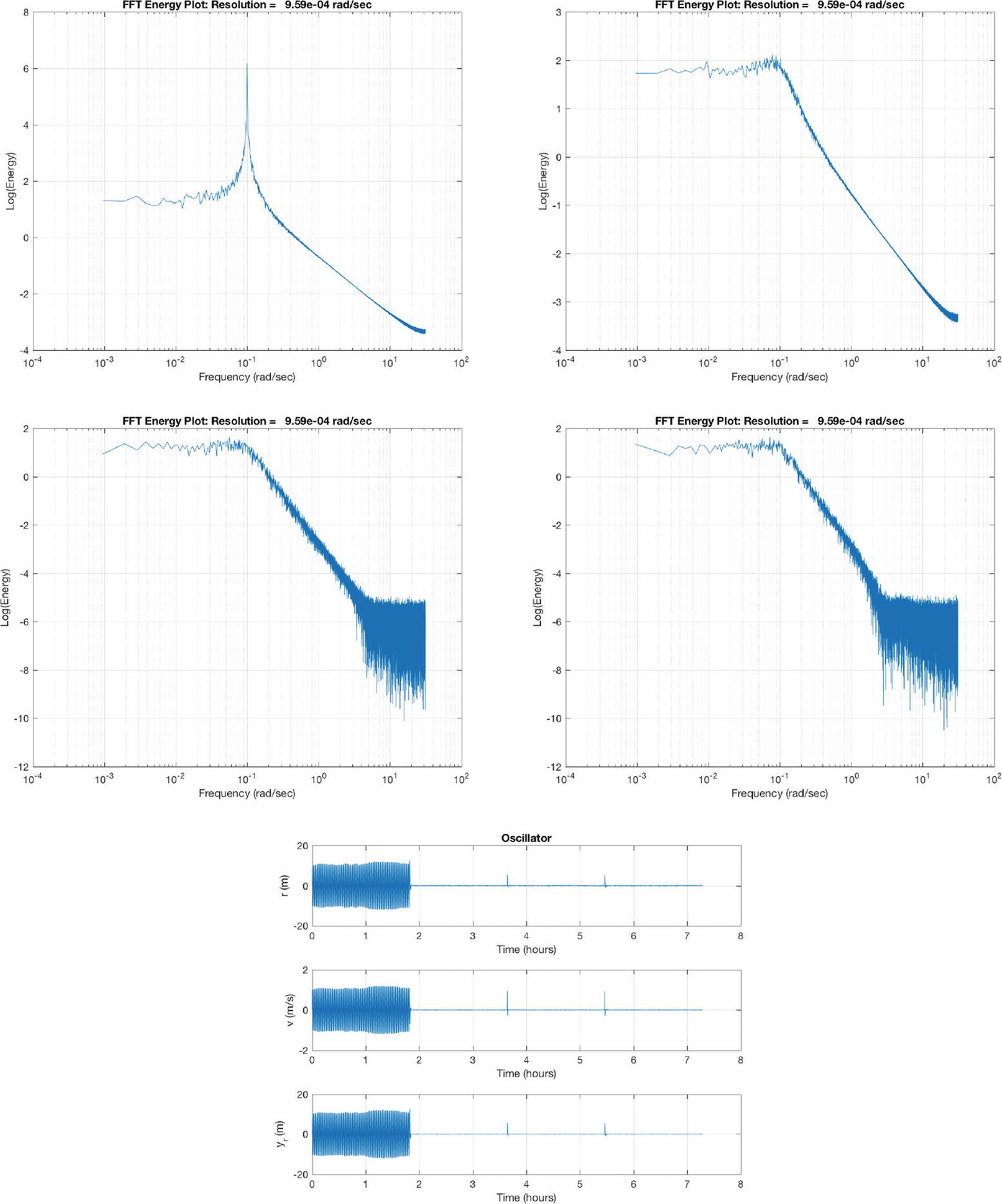
Tuning simulation results. The first four plots are the frequency spectrums taken at the end of each sampling interval; the last shows the results over time.
5.3 Implement Model Reference Adaptive Control


Speed control of a rotor for the Model Reference Adaptive Control demo.
5.3.1 Problem
We want to control a system to behave like a particular model. Our example is a simple rotor.
5.3.2 Solution
The solution is to implement an MRAC function.
5.3.3 How It Works
The idea is to have a dynamical model that defines the behavior of your system. You want your system to have the same dynamics. This desired model is the reference, hence the name Model Reference Adaptive Control. We will use the MIT rule [3] to design the adaptation system. The MIT rule was first developed at the MIT Instrumentation Laboratory (now Draper Laboratory), which developed the NASA Apollo and Space Shuttle guidance and control systems.


 . We then write:


Now that we have the MRAC controller done, we’ll write some supporting functions and then test it all out in RotorSim.
5.4 Generating a Square Wave Input
5.4.1 Problem
We need to generate a square wave to stimulate the rotor in the previous recipe.
5.4.2 Solution
For the purposes of simulation and testing our controller we will generate a square wave with a function.
5.4.3 How It Works
SquareWave generates a square wave. The first few lines are our standard code for running a demo or returning the data structure.
This function uses d.state to determine if it is in the high or low part of a square wave. The width of the low part of the wave is set in d.tLow. The width in the high part of the square wave is set in d.tHigh. It stores the time of the last switch in d.tSwitch.

Square wave.
We adjusted the y-axis limit and line width using the code:
TIP
h = get( gca,’children’) gives you access to the line data structure in a plot for the most recent axes.
5.5 Demonstrate MRAC for a Rotor
5.5.1 Problem
We want to create a recipe to control our rotor using MRAC.
5.5.2 Solution
The solution is to use implement our MRAC function in a MATLAB script from Recipe 5.3.
5.5.3 How It Works
Model Reference Adaptive Control is implemented in the script RotorSim. It calls MRAC to control the rotor. As in our other scripts, we use PlotSet for our 2D plots. Notice that we use two new options. One ’plot set’ allows you to put more than one line on a subplot. The other ’legend’ adds legends to each plot. The cell array argument to ’legend’ has a cell array for each plot. In this case, we have two plots each with two lines, so the cell array is:
Each plot legend is a cell entry within the overall cell array.
The rotor simulation script with MRAC is shown in the following listing. The square wave functions generates the command to the system that ω should track. RHSRotor, SquareWave, and MRAC all return default data structures. MRAC and SquareWave are called once per pass through the loop. The simulation right-hand side, that is the dynamics of the rotor, in RHSRotor, is then propagated using RungeKutta. Note that we pass a pointer to RHSRotor to RungeKutta.
TIP
Pass pointers @fun instead of strings ’fun’ to functions whenever possible.
RHSRotor is shown below.
The dynamics is just one line of code. The remaining returns the default data structure.
 .
.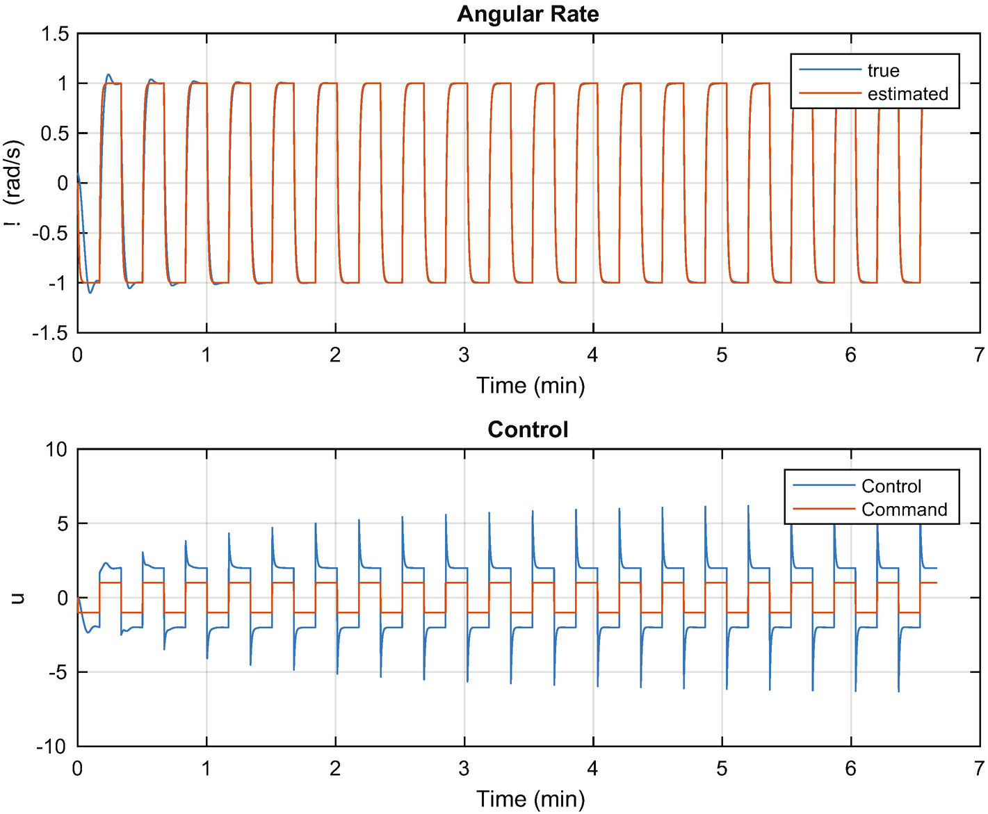
MRAC control of a rotor.
The first plot shows the estimated and true angular rates of the rotor on top and the control demand and actual control sent to the wheel on the bottom. The desired control is a square wave (generated by SquareWave). Notice the transient in the applied control at the transitions of the square wave. The control amplitude is greater than the commanded control. Notice also that the angular rate approaches the desired commanded square wave shape.
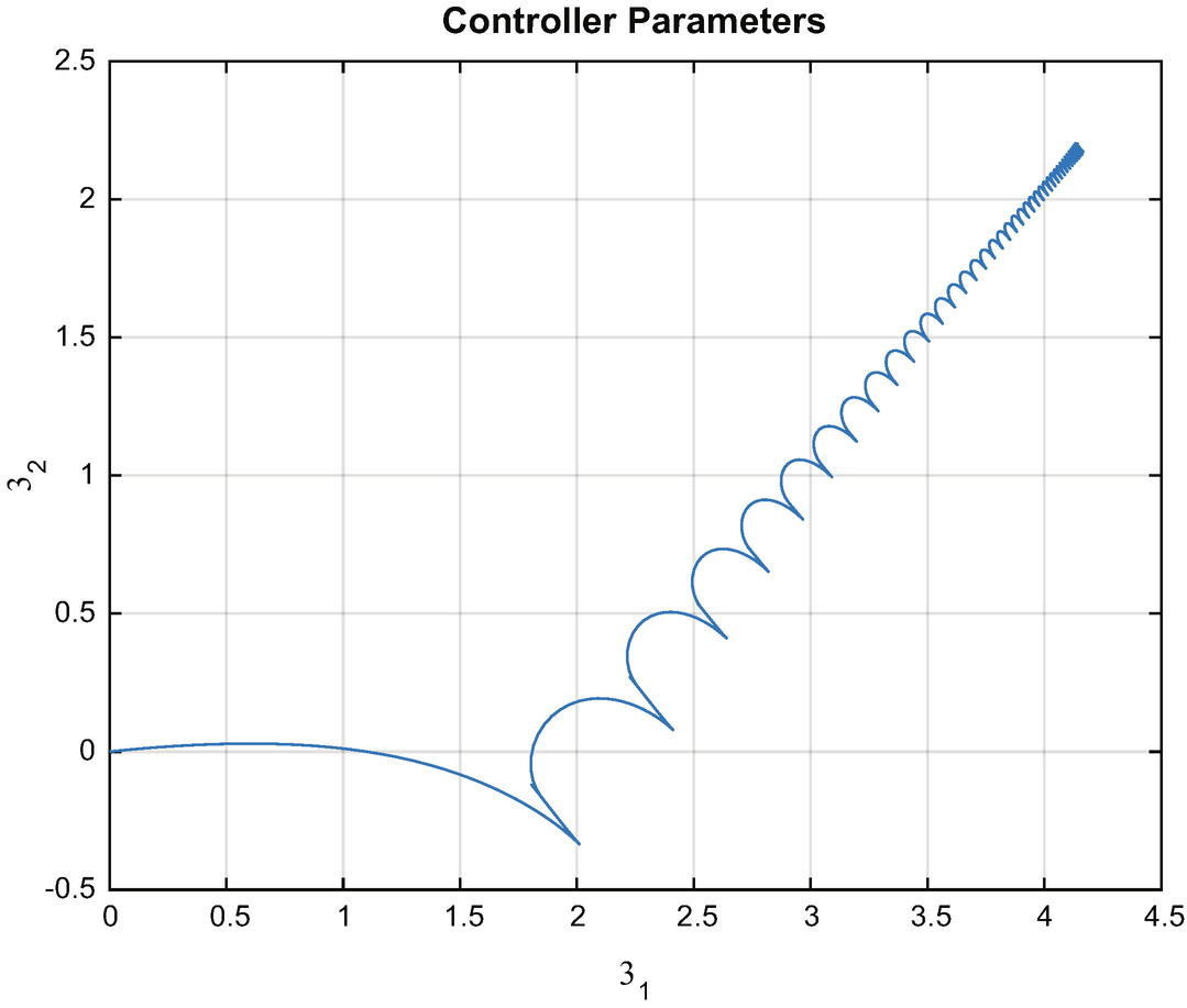
Gain convergence in the MRAC controller.
Model Reference Adaptive Control learns the gains of the system by observing the response to the control excitation. It requires excitation to converge. This is the nature of all learning systems. If there is insufficient stimulation, it isn’t possible to observe the behavior of the system, so there is not enough information for learning. It is easy to find an excitation for a first-order system. For higher order systems, or nonlinear systems, this can be more difficult.
5.6 Ship Steering: Implement Gain Scheduling for Steering Control of a Ship
5.6.1 Problem
We want to steer a ship at all speeds. The problem is that the dynamics are speed dynamics, making this a nonlinear problem
5.6.2 Solution
The solution is to use gain scheduling to set the gains based on speeds. The gain scheduling is learned by automatically computing gains from the dynamical equations of the ship. This is similar to the self-tuning example except that we are seeking a set of gains for all speeds, not just one. In addition, we assume that we know the model of the system.
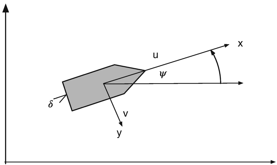
Ship heading control for gain scheduling control.
5.6.3 How It Works
![$$\displaystyle \begin{aligned} \left[ \begin{array}{l} \dot{v}\\ \dot{r}\\ \dot{\psi} \end{array} \right] = \left[ \begin{array}{rrr} \left(\frac{u}{l}\right)a_{11}&ua_{12}&0\\ \left(\frac{u}{l^2}\right)a_{21}&\left(\frac{u}{l}\right)a_{22}&0\\ 0&1&0 \end{array} \right] \left[ \begin{array}{l} v\\ r\\ \psi \end{array} \right] + \left[ \begin{array}{r} \left(\frac{u^2}{l}\right)b_1\\ \left(\frac{u^2}{l^2}\right)b_2\\ 0 \end{array} \right]\delta + \left[ \begin{array}{r} \alpha_v\\ \alpha_r\\ 0 \end{array} \right] \end{aligned} $$](../images/420697_2_En_5_Chapter/420697_2_En_5_Chapter_TeX_Equ40.png)
The disturbances only affect the dynamic states, r and v. The last state, ψ is a kinematic state and does not have a disturbance.
Ship Parameters [3]
Parameter | Minesweeper | Cargo | Tanker |
|---|---|---|---|
l | 55 | 161 | 350 |
a 11 | -0.86 | -0.77 | -0.45 |
a 12 | -0.48 | -0.34 | -0.44 |
a 21 | -5.20 | -3.39 | -4.10 |
a 22 | -2.40 | -1.63 | -0.81 |
b 1 | 0.18 | 0.17 | 0.10 |
b 2 | 1.40 | -1.63 | -0.81 |
In the ship simulation, ShipSim, we linearly increase the forward speed while commanding a series of heading psi changes. The controller takes the state space model at each time step and computes new gains, which are used to steer the ship. The controller is a linear quadratic regulator. We can use full state feedback because the states are easily modeled. Such controllers will work perfectly in this case, but are a bit harder to implement when you need to estimate some of the states or have unmodeled dynamics.
The quadratic regulator generator code is shown in the following lists. It generates the gain from the matrix Riccati equation. A Riccati equation is an ordinary differential equation that is quadratic in the unknown function. In steady state, this reduces to the algebraic Riccati equation, which is solved in this function.
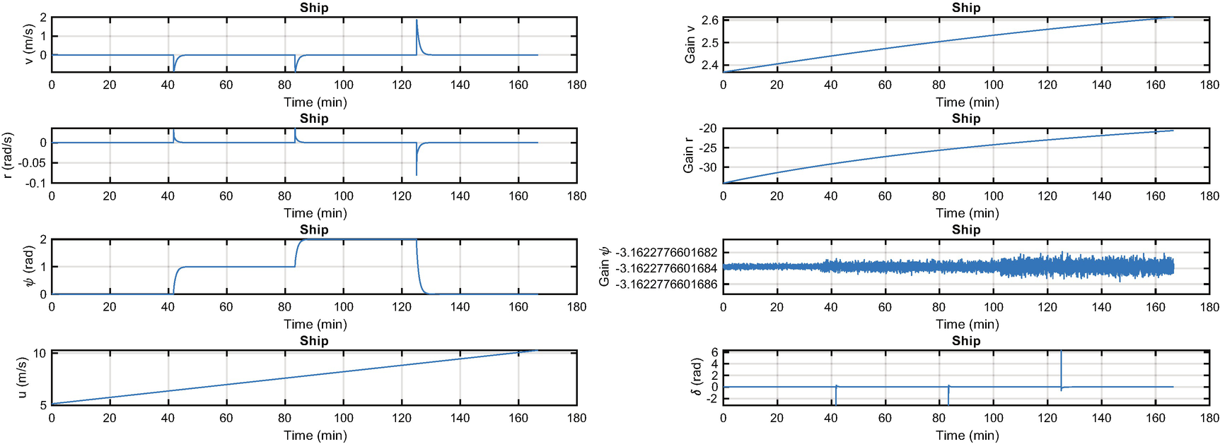
Ship steering simulation. The states are shown on the left with the forward velocity. The gains and rudder angle are shown on the right. Notice the “pulses” in the rudder to make the maneuvers.
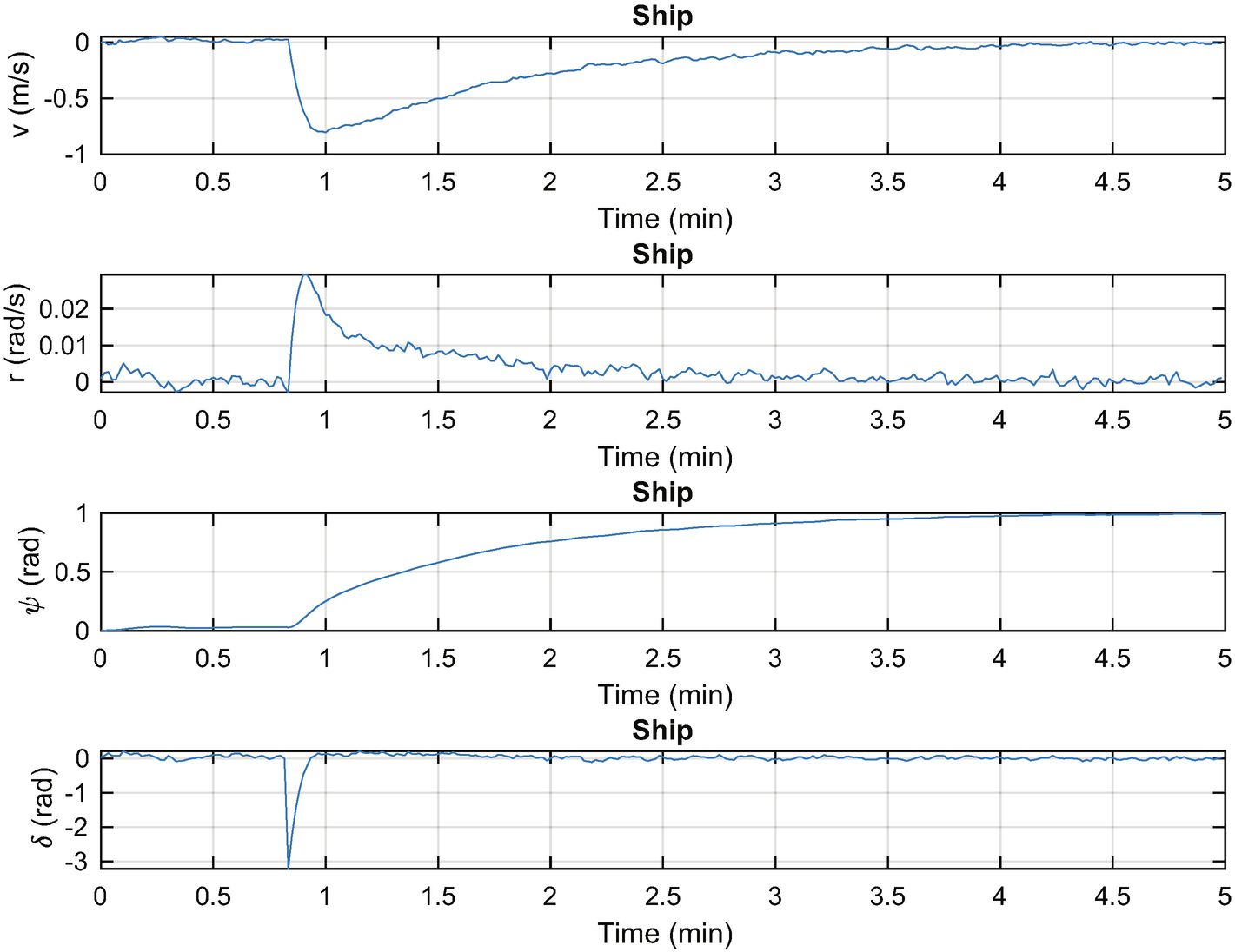
Ship steering simulation. The states are shown on the left with the rudder angle. The disturbances are Gaussian white noise.
5.7 Spacecraft Pointing
5.7.1 Problem
We want to control the orientation of a spacecraft with thrusters for control.
5.7.2 Solution
The solution is to use a parameter estimator to estimate the inertia and feed it into the control system.
5.7.3 How It Works
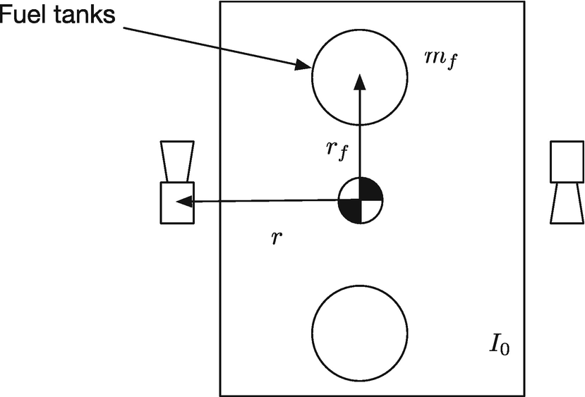
Spacecraft model.


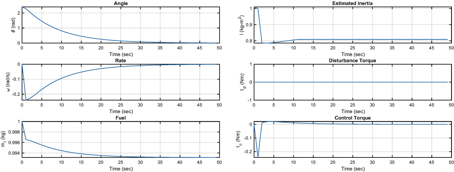
States and control outputs from the spacecraft simulation.
This algorithm appears crude, but it is fundamentally all we can do in this situation given just angular rate measurements. More sophisticated filters or estimators could improve the performance.
5.8 Summary
Chapter Code Listing
File | Description |
|---|---|
Combinations | Enumerates n integers for 1:n taken k at a time. |
FFTEnergy | Generates fast Fourier transform energy. |
FFTSim | Demonstration of the fast Fourier transform. |
MRAC | Implement model reference adaptive control. |
QCR | Generates a full state feedback controller. |
RHSOscillatorControl | Right-hand side of a damped oscillator with a velocity gain. |
RHSRotor | Right-hand side for a rotor. |
RHSShip | Right-hand side for a ship steering model. |
RHSSpacecraft | Right-hand side for a spacecraft model. |
RotorSim | Simulation of model reference adaptive control. |
ShipSim | Simulation of ship steering. |
ShipSimDisturbance | Simulation of ship steering with disturbances. |
SpacecraftSim | Time varying inertia demonstration. |
SquareWave | Generate a square wave. |
TuningSim | Controller tuning demonstration. |
WrapPhase | Keep angles between − π and π. |