
In Chapter 7, we looked at a traditional neural network (NN). One of the limitations of a traditional NN is that it is not translation invariant—that is, a cat image on the upper right-hand corner of an image would be treated differently from an image that has a cat in the center of the image. Convolutional neural networks (CNNs) are used to deal with such issues.
Given that a CNN can deal with translation in images, it is considered a lot more useful and CNN architectures are in fact among the current state-of-the-art techniques in object classification/detection.
Working details of CNN
How CNN improves over the drawbacks of neural network
The impact of convolutions and pooling on addressing image translation issues
How to implement CNN in Python, and R
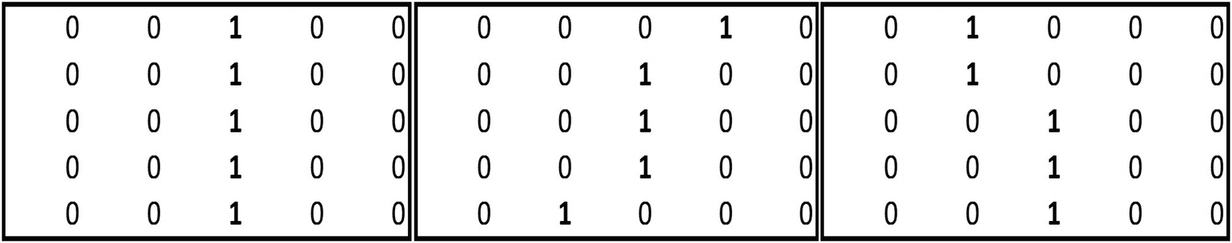
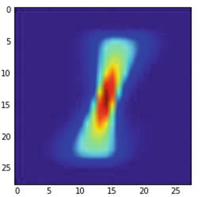
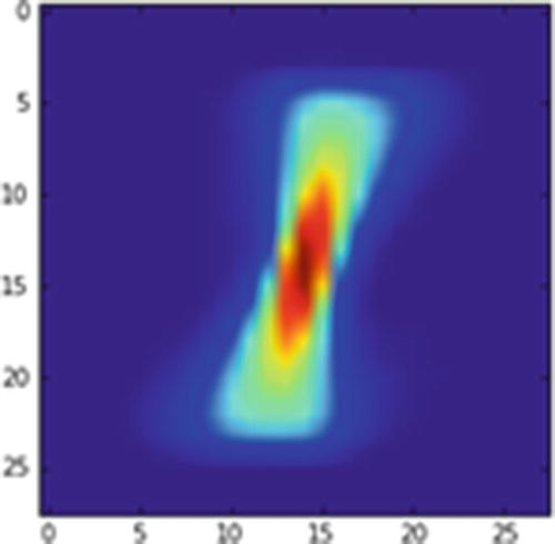
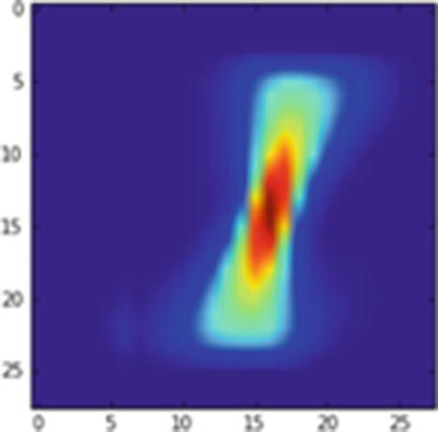
Image of pixels corresponding to images with label 1
In the image, the redder the pixel, the more often have people written on top of it; bluer means the pixel had been written on fewer times. The pixel in middle is the reddest, quite likely because most people would be writing over that pixel, regardless of the angle they use to write a 1—a vertical line or slanted towards the left or right. In the following section, you would notice that the neural network predictions are not accurate when the image is translated by a few units. In a later section, we will understand how CNN addresses the problem of image translation.
The Problem with Traditional NN
In the scenario just mentioned, a traditional neural network would highlight the image as a 1 only if the pixels around the middle are highlighted and the rest of the pixels in the image are not highlighted (since most people have highlighted the pixels in the middle).
- 1.
Download the dataset and extract the train and test datasets:
from keras.datasets import mnistimport matplotlib.pyplot as plt%matplotlib inline# load (downloaded if needed) the MNIST dataset(X_train, y_train), (X_test, y_test) = mnist.load_data()# plot 4 images as gray scaleplt.subplot(221)plt.imshow(X_train[0], cmap=plt.get_cmap('gray'))plt.subplot(222)plt.imshow(X_train[1], cmap=plt.get_cmap('gray'))plt.subplot(223)plt.imshow(X_train[2], cmap=plt.get_cmap('gray'))plt.subplot(224)plt.imshow(X_train[3], cmap=plt.get_cmap('gray'))# show the plotplt.show()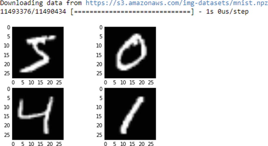
- 2.
Import the relevant packages:
import numpy as npfrom keras.datasets import mnistfrom keras.models import Sequentialfrom keras.layers import Densefrom keras.layers import Dropoutfrom keras.layers import Flattenfrom keras.layers.convolutional import Conv2Dfrom keras.layers.convolutional import MaxPooling2Dfrom keras.utils import np_utilsfrom keras import backend as K - 3.
Fetch the training set corresponding to the label 1 only:
X_train1 = X_train[y_train==1] - 4.
Reshape and normalize the dataset:
num_pixels = X_train.shape[1] * X_train.shape[2]X_train = X_train.reshape(X_train.shape[0],num_pixels ).astype('float32')X_test = X_test.reshape(X_test.shape[0],num_pixels).astype('float32')X_train = X_train / 255X_test = X_test / 255 - 5.
One-hot-encode the labels:
y_train = np_utils.to_categorical(y_train)y_test = np_utils.to_categorical(y_test)num_classes = y_train.shape[1] - 6.
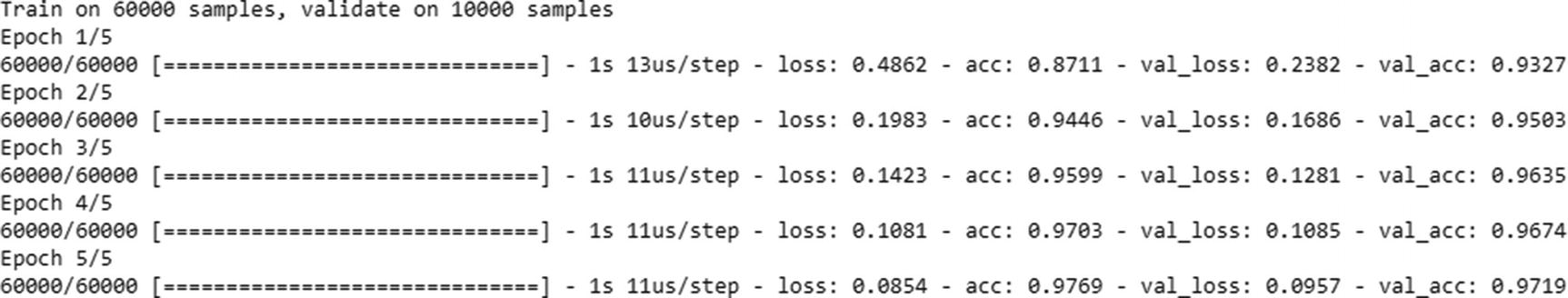
Build a model and run it:
model = Sequential()model.add(Dense(1000, input_dim=num_pixels, activation="relu"))model.add(Dense(num_classes, activation="softmax"))model.compile(loss='categorical_crossentropy', optimizer="adam", metrics=[''accuracy'])model.fit(X_train, y_train, validation_data=(X_test, y_test), epochs=5, batch_size=1024, verbose=1)
Let’s plot what an average 1 label looks like:
Average 1 image
Scenario 1
In this scenario, a new image is created (Figure 9-3) in which the original image is translated by 1 pixel toward the left:
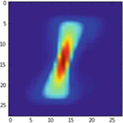
Average 1 image translated by 1 pixel to the left
Let’s go ahead and predict the label of the image in Figure 9-3 using the built model:

We see the wrong prediction of 8 as output.
Scenario 2
A new image is created (Figure 9-4) in which the pixels are not translated from the original average 1 image:
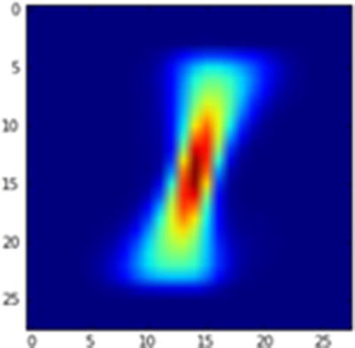
Average 1 image
The prediction of this image is as follows:

We see a correct prediction of 1 as output.
Scenario 3
A new image is created (Figure 9-5) in which the pixels of the original average 1 image are shifted by 1 pixel to the right:
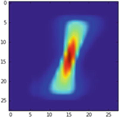
Average 1 image translated by 1 pixel to the right
Let us go ahead and predict the label of the above image using the built model:

We have a correct prediction of 1 as output.
Scenario 4
A new image is created (Figure 9-6) in which the pixels of the original average 1 image are shifted by 2 pixels to the right:
Average 1 image translated by 2 pixels to the right
We’ll predict the label of the image using the built model:

And we see a wrong prediction of 3 as output.
From the preceding scenarios, you can see that traditional NN fails to produce good results the moment there is translation in the data. These scenarios call for a different way of dealing with the network to address translation variance. And this is where a convolutional neural network (CNN) comes in handy.
Understanding the Convolutional in CNN
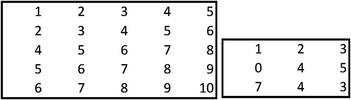
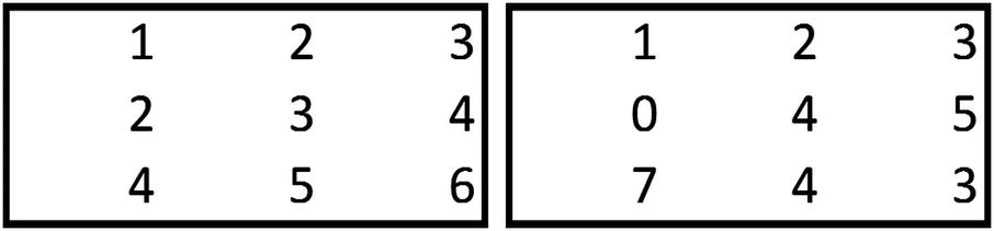
You already have a good idea of how a typical neural network works. In this section, let’s explore what the word convolutional means in CNN. A convolution is a multiplication between two matrices, with one matrix being big and the other smaller.
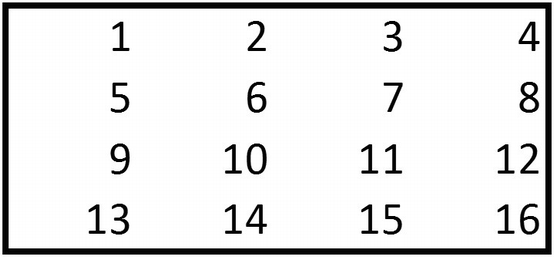
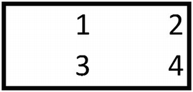
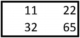
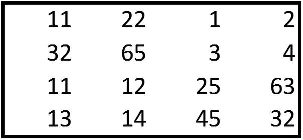
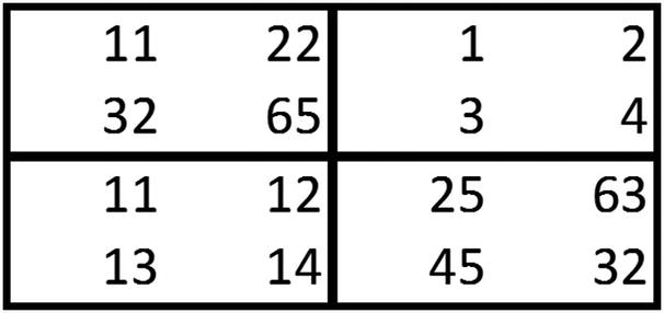
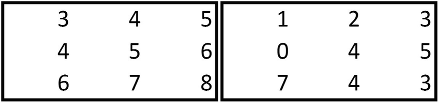
To see convolution, consider the following example.
- 1.
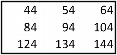
{1,2,5,6} of the bigger matrix is multiplied with {1,2,3,4} of the smaller matrix.
1 × 1 + 2 × 2 + 5 × 3 + 6 × 4 = 44
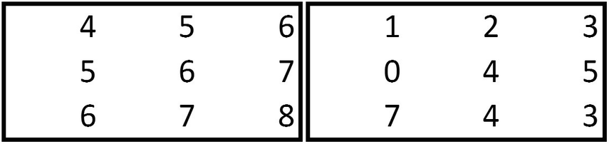
- 2.
{2,3,6,7} of the bigger matrix is multiplied with {1,2,3,4} of the smaller matrix:
2 × 1 + 3 × 2 + 6 × 3 + 7 × 4 = 54
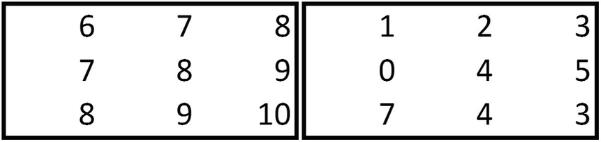
- 3.
{3,4,7,8} of the bigger matrix is multiplied with {1,2,3,4} of the smaller matrix:
3 × 1 + 4 × 2 + 7 × 3 + 8 × 4 = 64
- 4.
{5,6,9,10} of the bigger matrix is multiplied with {1,2,3,4} of the smaller matrix:
5 × 1 + 6 × 2 + 9 × 3 + 10 × 4 = 84
- 5.
{6,7,10,11} of the bigger matrix is multiplied with {1,2,3,4} of the smaller matrix:
6 × 1 + 7 × 2 + 10 × 3 + 11 × 4 = 94
- 6.
{7,8,11,12} of the bigger matrix is multiplied with {1,2,3,4} of the smaller matrix:
7 × 1 + 8 × 2 + 11 × 3 + 12 × 4 = 104
- 7.
{9,10,13,14} of the bigger matrix is multiplied with {1,2,3,4} of the smaller matrix:
9 × 1 + 10 × 2 + 13 × 3 + 14 × 4 = 124
- 8.
{10,11,14,15} of the bigger matrix is multiplied with {1,2,3,4} of the smaller matrix:
10 × 1 + 11 × 2 + 14 × 3 + 15 × 4 = 134
- 9.
{11,12,15,16} of the bigger matrix is multiplied with {1,2,3,4} of the smaller matrix:
11 × 1 + 12 × 2 + 15 × 3 + 16 × 4 = 144
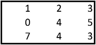
Conventionally, the smaller matrix is called a filter or kernel, and the smaller matrix values are arrived at statistically through gradient descent (more on gradient descent a little later). The values within the filter can be considered as the constituent weights.
From Convolution to Activation
In a traditional NN, a hidden layer not only multiplies the input values by the weights, but also applies a non-linearity to the data—it passes the values through an activation function. A similar activity happens in a typical CNN too, where the convolution is passed through an activation function. CNN supports the traditional activations functions we have seen so far: sigmoid, ReLU, Tanh.
For the preceding output, note that the output remains the same when passed through a ReLU activation function , as all the numbers are positive.
From Convolution Activation to Pooling
So far, we have looked at how convolutions work. In this section, we will consider the typical next step after a convolution: pooling.
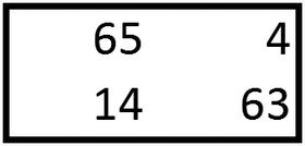
Note that, in practice, it is not necessary to always have a 2 × 2 filter.
The other types of pooling involved are sum and average. Again, in practice we see a lot of max pooling when compared to other types of pooling.
How Do Convolution and Pooling Help?
One of the drawbacks of traditional NN in the MNIST example we looked at earlier was that each pixel is associated with a distinct weight. Thus, if an adjacent pixel other than the original pixel became highlighted, the output would not be very accurate (the example of scenario 1, where the 1s were slightly to the left of the middle).
This scenario is now addressed, as the pixels share weights that are constituted within each filter. All the pixels are multiplied by all the weights that constitute a filter, and in the pooling layer only the values that are activated the highest are chosen. This way, regardless of whether the highlighted pixel is at the center or is slightly away from the center, the output would more often than not be the expected value. However, the issue remains the same when the highlighted pixels are far away from the center.
Creating CNNs with Code
From the preceding traditional NN scenario, we saw that a NN does not work if the pixels are translated by 1 unit to the left. Practically, we can consider the convolution step as identifying the pattern and pooling step as the one that results in translation variance.
- 1.
Import and reshape the data to fit a CNN:
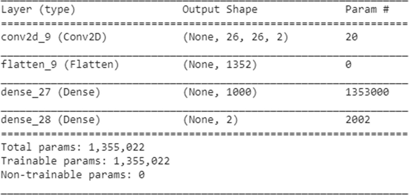
(X_train, y_train), (X_test, y_test) = mnist.load_data()X_train = X_train.reshape(X_train.shape[0],X_train.shape[1],X_train.shape[1],1 ).astype('float32')X_test = X_test.reshape(X_test.shape[0],X_test.shape[1],X_test.shape[1],1).astype('float32')X_train = X_train / 255X_test = X_test / 255y_train = np_utils.to_categorical(y_train)y_test = np_utils.to_categorical(y_test)num_classes = y_test.shape[1]Step 2: Build a modelmodel = Sequential()model.add(Conv2D(10, (3,3), input_shape=(28, 28,1), activation="relu"))model.add(MaxPooling2D(pool_size=(2, 2)))model.add(Flatten())model.add(Dense(1000, activation="relu"))model.add(Dense(num_classes, activation="softmax"))model.compile(loss='categorical_crossentropy', optimizer="adam", metrics=['accuracy'])model.summary()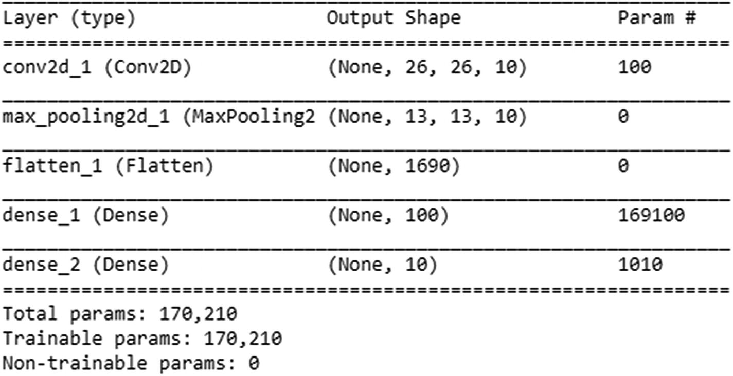
- 2.
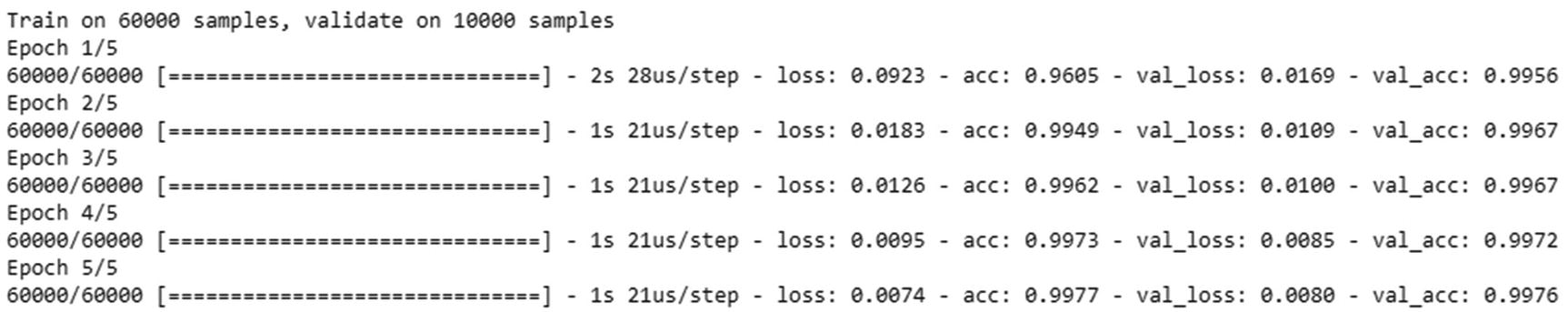
Fit the model:
model.fit(X_train, y_train, validation_data=(X_test, y_test), epochs=5, batch_size=1024, verbose=1)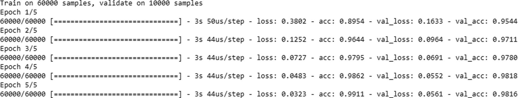
For the preceding convolution, where one convolution is followed by one pooling layer, the output prediction works out well if the pixels are translated by 1 unit to the left or right, but does not work when the pixels are translated by more than 1 unit (Figure 9-7):
Average 1 image translated by 1 pixel to the left
Let’s go ahead and predict the label of Figure 9-7:

We see a correct prediction of 1 as output.
In the next scenario (Figure 9-8), we move the pixels by 2 units to the left:
Average 1 image translated by 2 pixels to the left
Let’s predict the label of Figure 9-8 per the CNN model we built earlier:

We have an incorrect prediction when the image is translated by 2 pixels to the left.
Note that when the number of convolution pooling layers in the model is the same as the amount of translation in an image, the prediction is correct. But prediction is more likely to be incorrect if there are less convolution pooling layers when compared to the translation in image.
Working Details of CNN
- 1.
Import the relevant packages:
# import relevant packagesfrom keras.datasets import mnistimport matplotlib.pyplot as plt%matplotlib inlineimport numpy as npfrom keras.datasets import mnistfrom keras.models import Sequentialfrom keras.layers import Densefrom keras.layers import Dropoutfrom keras.utils import np_utilsfrom keras.layers import Flattenfrom keras.layers.convolutional import Conv2Dfrom keras.layers.convolutional import MaxPooling2Dfrom keras.utils import np_utilsfrom keras import backend as Kfrom keras import regularizers - 2.
Create a simple dataset:
# Create a simple datasetX_train=np.array([[[1,2,3,4],[2,3,4,5],[5,6,7,8],[1,3,4,5]],[[-1,2,3,-4],[2,-3,4,5],[-5,6,-7,8],[-1,-3,-4,-5]]])y_train=np.array([0,1]) - 3.
Normalize the inputs by dividing each value with the maximum value in the dataset:
X_train = X_train / 8 - 4.
One-hot-encode the outputs:
y_train = np_utils.to_categorical(y_train) - 5.
Once the simple dataset of just two inputs that are 4 × 4 in size and the two outputs are in place, let’s first reshape the input into the required format (which is: number of samples, height of image, width of image, number of channels of the image):
X_train = X_train.reshape(X_train.shape[0],X_train.shape[1],X_train.shape[1],1 ).astype('float32') - 6.
Build a model:
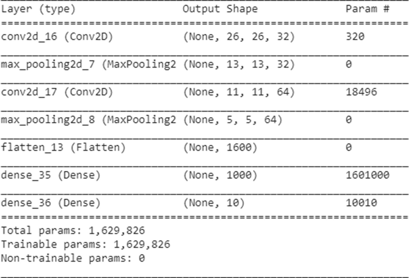
model = Sequential()model.add(Conv2D(1, (3,3), input_shape=(4,4,1), activation="relu"))model.add(MaxPooling2D(pool_size=(2, 2)))model.add(Flatten())model.add(Dense(10, activation="relu"))model.add(Dense(2, activation="softmax"))model.compile(loss='categorical_crossentropy', optimizer="adam", metrics=['accuracy'])model.summary()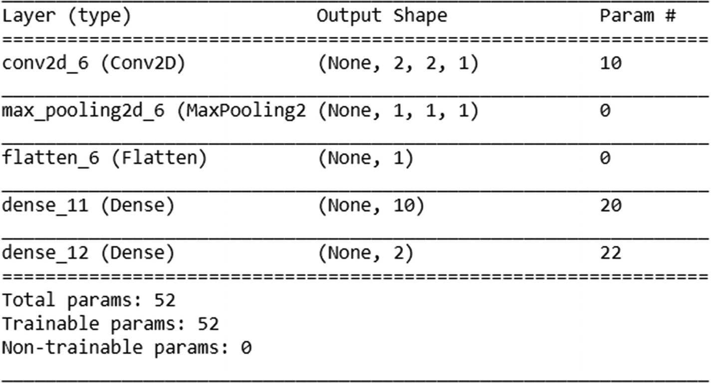
- 7.
Fit the model:
model.fit(X_train, y_train, epochs=100, batch_size=2, verbose=1)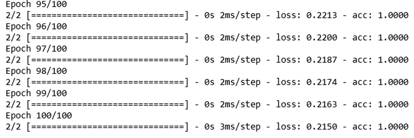
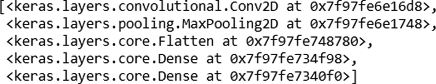
The various layers of the preceding model are as follows:
The name and shape corresponding to various layers are as follows:
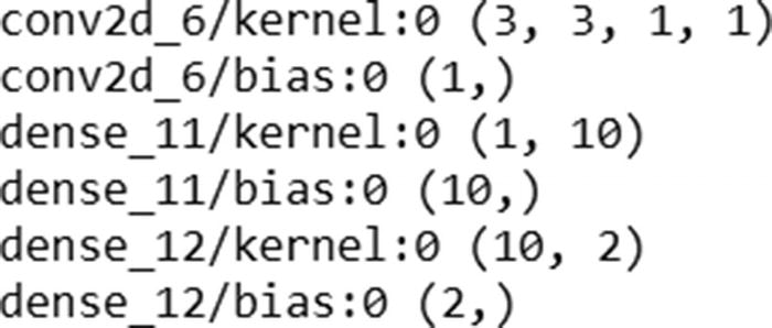
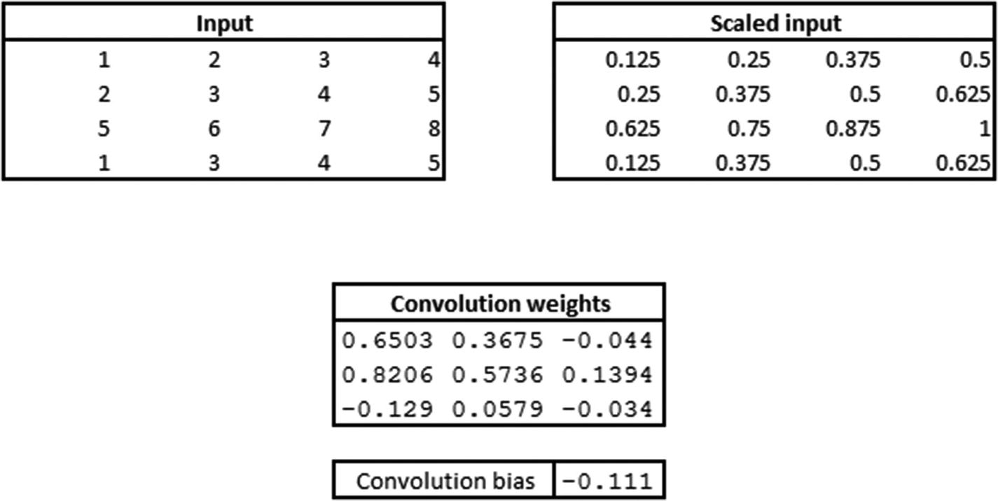
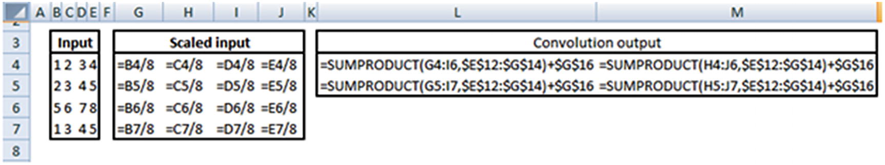
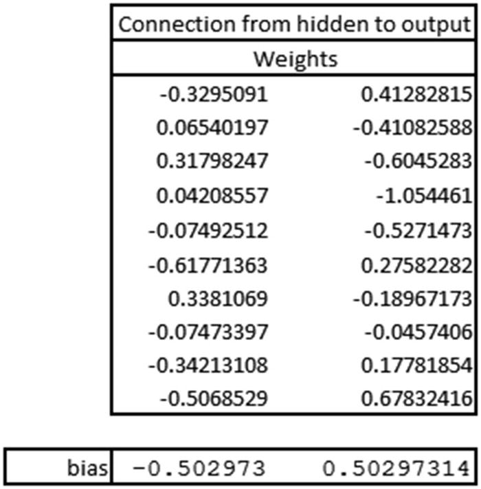
The weights corresponding to a given layer can be extracted as follows:
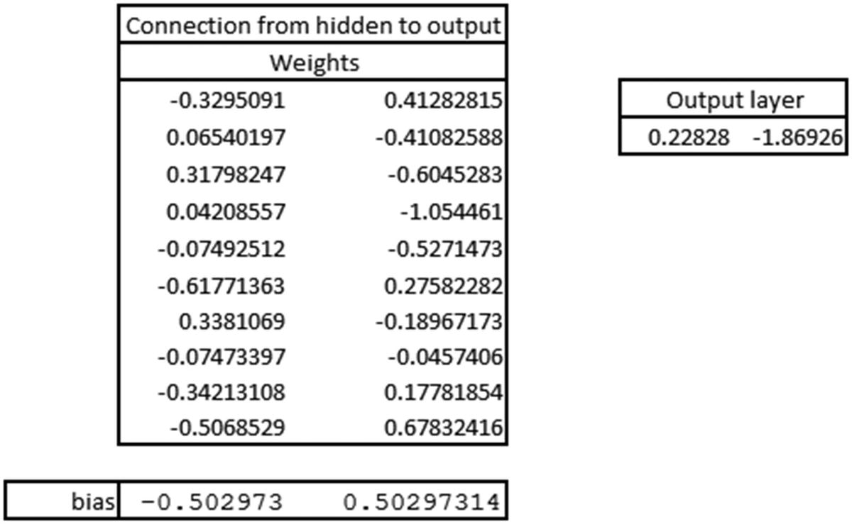
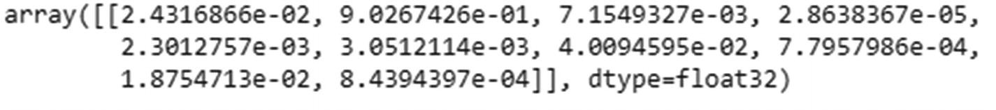
The prediction for the first input can be calculated as follows:

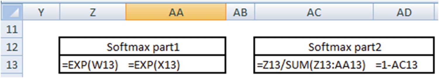
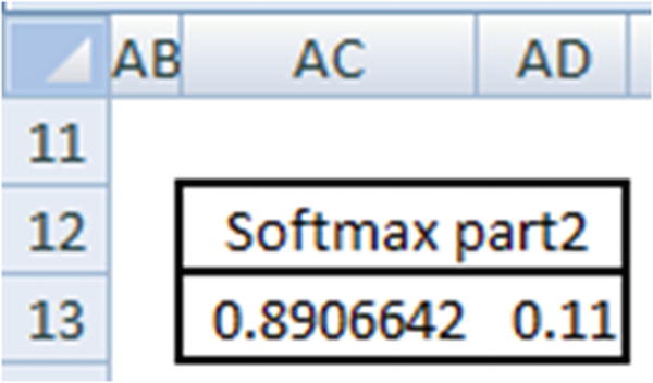
Now that we know the probability of 0 for the preceding prediction is 0.89066, let’s validate our intuition of CNN so far by matching the preceding prediction in Excel (available as “CNN simple example.xlsx” in github).
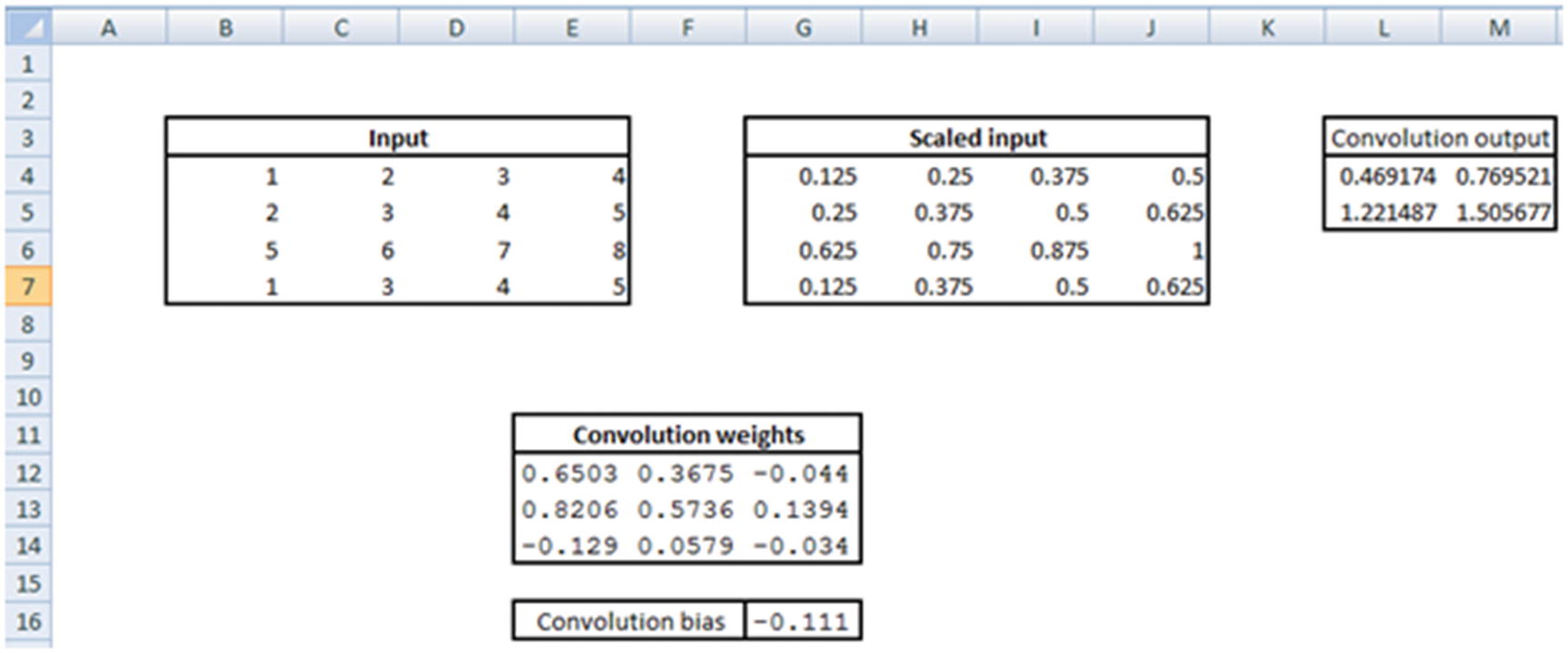
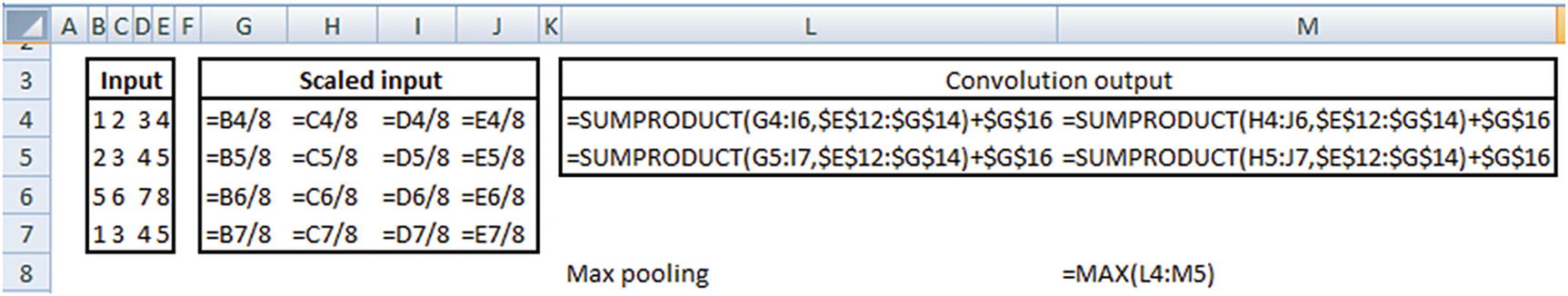
Once the pooling is performed, all the outputs are flattened (per the specification in our model). However, given that our pooling layer has only one output, flattening would also result in a single output.
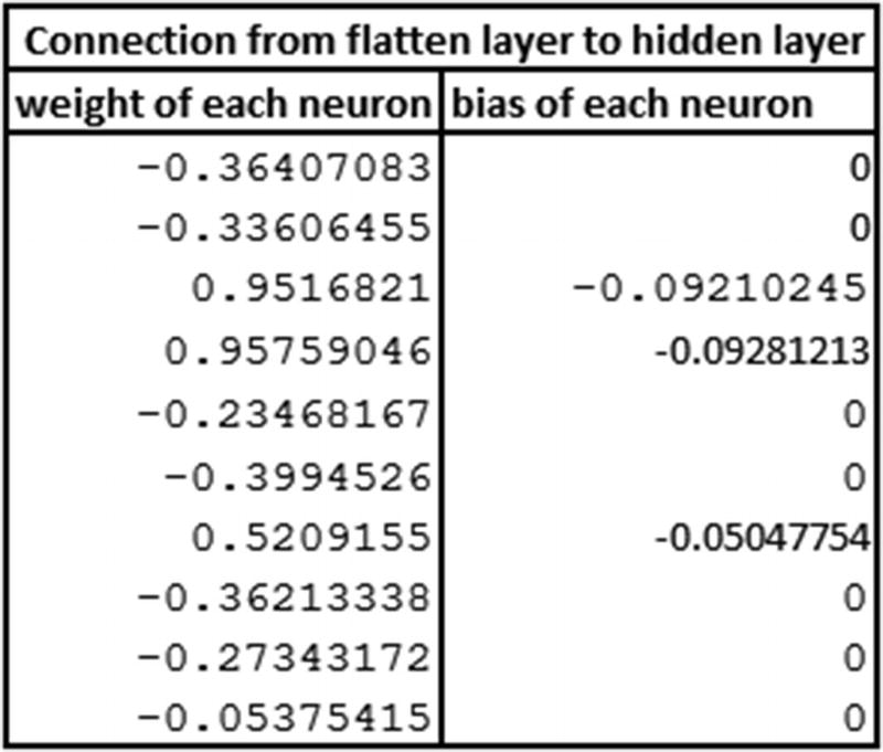
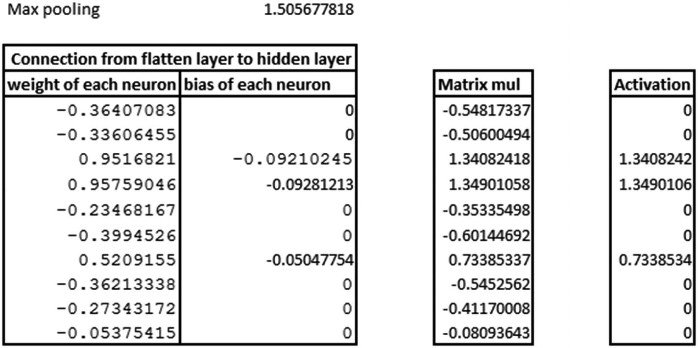
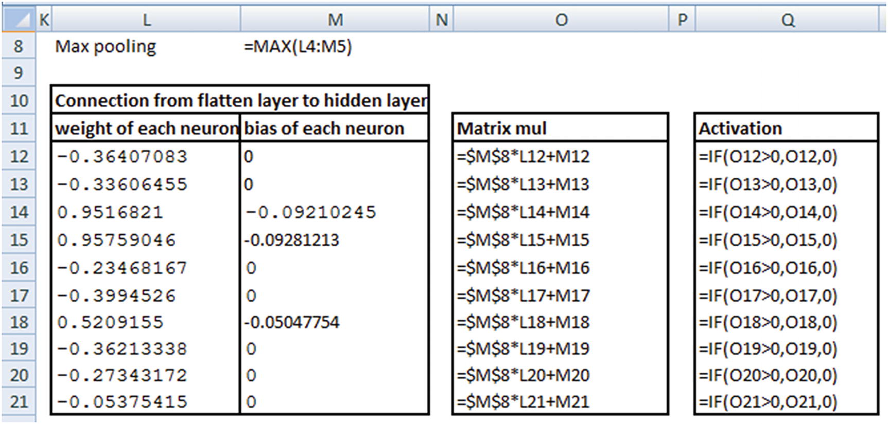
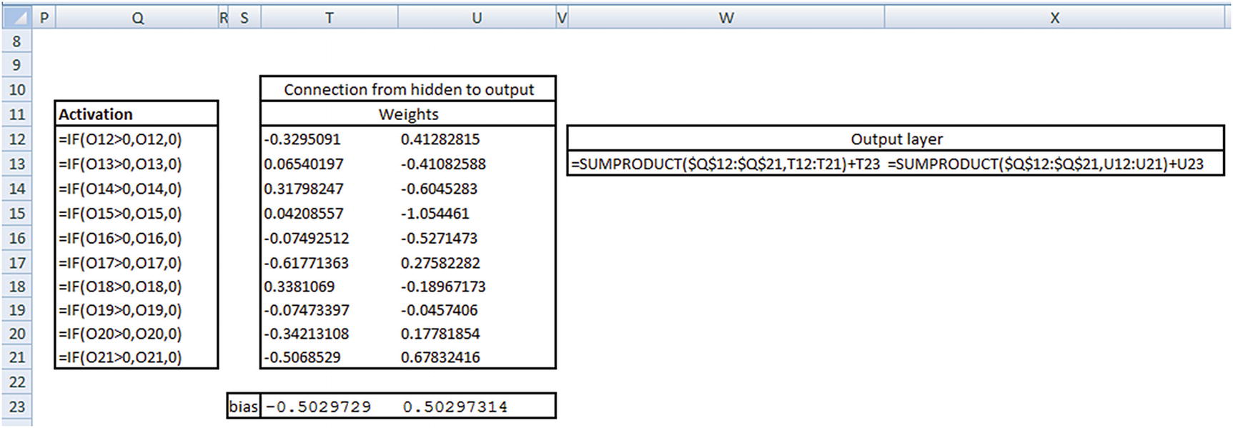
Thus, we have a validation about the intuition laid out in the previous sections.
Deep Diving into Convolutions/Kernels
To see how kernels/filters help, let’s go through another scenario. From the MNIST dataset, let’s modify the objective in such a way that we are only interested in predicting whether an image is a 1 or not a 1:
We will come up with a simple CNN where there are only two convolution filters:
Now we’ll go ahead and run the model as follows:
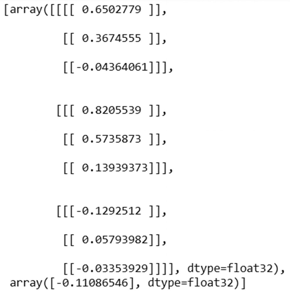
We can extract the weights corresponding to the filters in the following way:
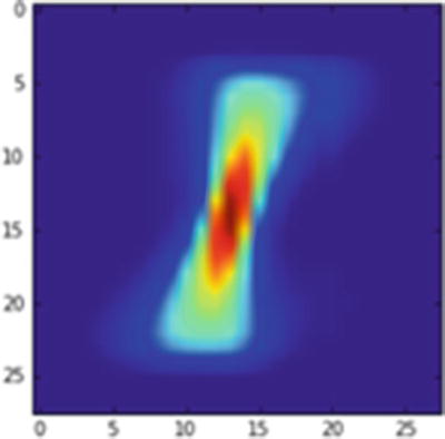
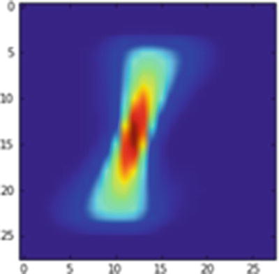
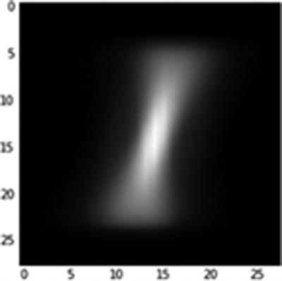
Let’s manually convolve and apply the activation by using the weights derived in the preceding step (Figure 9-9):
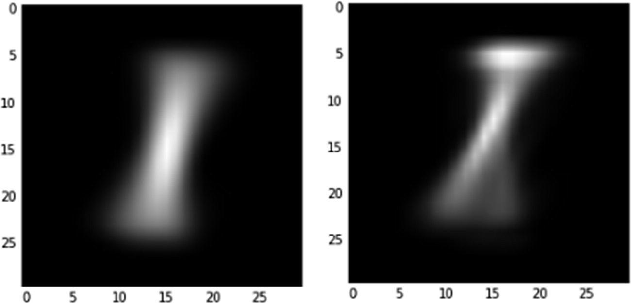
Average filter activations when 1 label images are passed
In the figure, note that the filter on the left activates a 1 image a lot more than the filter on the right. Essentially, the first filter helps in predicting label 1 more, and the second filter augments in predicting the rest.
From Convolution and Pooling to Flattening: Fully Connected Layer
The outputs we have seen so far until pooling layer are images . In traditional neural network, we would consider each pixel as an independent variable. This is precisely what we are going to perform in the flattening process .

From One Fully Connected Layer to Another
In a typical neural network, the input layer is connected to the hidden layer. In a similar manner, in a CNN the fully connected layer is connected to another fully connected layer that typically has more units.
From Fully Connected Layer to Output Layer
Similar to the traditional NN architecture, the hidden layer is connected to the output layer and is passed through a sigmoid activation to get the output as a probability. An appropriate loss function is also chosen, depending on the problem being solved.
Connecting the Dots: Feed Forward Network
- 1.
Convolution
- 2.
Pooling
- 3.
Flattening
- 4.
Hidden layer
- 5.
Calculating output probability
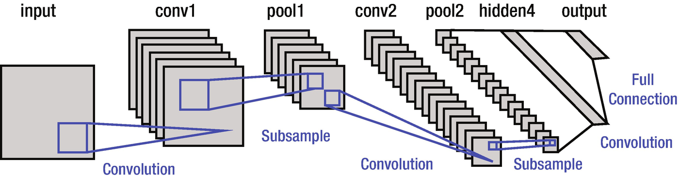
A typical CNN looks is shown in Figure 9-10 (the most famous—the one developed by the inventor himself, LeNet, as an example):
The subsample written in Figure 9-10 is equivalent to the max pooling step we saw earlier.
Other Details of CNN
A LeNet
- 1.
Let’s say we have a greyscale image that is 28 × 28 in dimension. Six filters that are 3 × 3 in size would generate images that are 26 × 26 in size. Thus, we are left with six images of size 26 × 26.
- 2.
A typical color image would have three channels (RGB). For simplicity, we can assume that the output image we had in step 1 has six channels - one each for the six filters (though we can’t name them as RGB like the three-channel version). In this step, we would perform max pooling on each of the six channels separately. This would result in six images (channels) that are 13 × 13 in dimension.
- 3.
In the next convolution step, we multiply the six channels of 13 × 13 images with weights of dimensions 3 × 3 × 6. That’s a 3-dimensional weight matrix convolving over a 3-dimensional image (where the image has dimensions 13 × 13 × 6). This would result in an image of 11 × 11 in dimension for each filter.
Let’s say we’ve considered ten different weight matrices (cubes, to be precise). This would result in an image that is 11 × 11 × 10 in dimension.
- 4.
Max pooling on each of the 11 × 11 images (which are ten in number) would result in a 5 × 5 image. Note that, when the max pooling is performed on an image that has odd number of dimensions, pooling gives us the rounded-down image—that is, 11/2 is rounded down to 5.
Note that the output of the convolution is a 2 × 2 matrix when the stride is 2 for the matrices of the given dimensions here.
Padding
Note that the size of the resulting image is reduced when a convolution is performed on top of it. One way to get rid of the size-reduction issue is to pad the original image with zeroes on the four borders. This way, a 28 × 28 image would be translated into a 30 × 30 image. Thus, when the 30 × 30 image is convolved by a 3 × 3 filter, the resulting image would be a 28 × 28 image.
Backward Propagation in CNN
Backward propagation in CNN is done in similarly to a typical NN, where the impact of changing a weight by a small amount on the overall weight is calculated. But in place of weights, as in NN, we have filters/matrices of weights that need to be updated to minimize the overall loss.
Sometimes, given that there are typically millions of parameters in a CNN, having regularization can be helpful. Regularization in CNN can be achieved using the dropout method or the L1 and L2 regularizations. Dropout is done by choosing not to update some weights (typically a randomly chosen 20% of total weights) and training the entire network over the whole number of epochs .
Putting It All Together
The following code implements a three-convolution pooling layer followed by flattening and a fully connected layer:
In the next step, we build the model, as follows:
Finally, we fit the model, as follows:
Note that the accuracy of the model trained using the preceding code is ~98.8%. But note that although this model works best on the test dataset, an image that is translated or rotated from the test MNIST dataset would not be classified correctly (In general, CNN could only help when the image is translated by the number of convolution pooling layers). That can be verified by looking at the prediction when the average 1 image is translated by 2 pixels to the left once, and in another scenario, 3 pixels to the left, as follows:
Note that, in this case, where the image is translated by 2 units to the left, the predictions are accurate:

Note that here, when the image is translated by more pixels than convolution pooling layers, the prediction is not accurate. This issue is solved by using data augmentation, the topic of the next section.
Data Augmentation
Technically, a translated image is the same as a new image that is generated from the original image . New data can be generated by using the ImageDataGenerator function in keras:
From that code, we have generated 50,000 random shufflings from our original data , where the pixels are shuffled by 20%.
As we plot the image of 1 now (Figure 9-11), note that there is a wider spread for the image:
Average 1 post data augmentation
Now the predictions will work even when we don’t do convolution pooling for the few pixels that are to the left or right of center. However, for the pixels that are far away from the center, correct predictions will come once the model is built using the convolution and pooling layers.
So, data augmentation helps in further generalizing for variations of the image across the image boundaries when using the CNN model, even with fewer convolution pooling layers.
Implementing CNN in R
To implement CNN in R, we will leverage the same package we used to implement neural network in R—kerasR (code available as “kerasr_cnn_code.r” in github):
The preceding code results in an accuracy of ~97%.
Summary
In this chapter, we saw how convolutions help us identify the structure of interest and how pooling helps ensure that the image is recognized even when translation happens in the original image. Given that CNN is able to adapt to image translation through convolution and pooling, it’s in a position to give better results than the traditional neural network.