Word2vec is a neural network–based approach that comes in very handy in traditional text mining analysis.
One of the problems with a traditional text mining approach is an issue with the dimensionality of data. Given the high number of distinct words within a typical text, the number of columns that are built can become very high (where each column corresponds to a word, and each value in the column specifies whether the word exists in the text corresponding to the row or not—more about this later in the chapter).
Word2vec helps represent data in a better way: words that are similar to each other have similar vectors, whereas words that are not similar to each other have different vectors. In this chapter, we will explore the different ways in which word vectors are calculated.
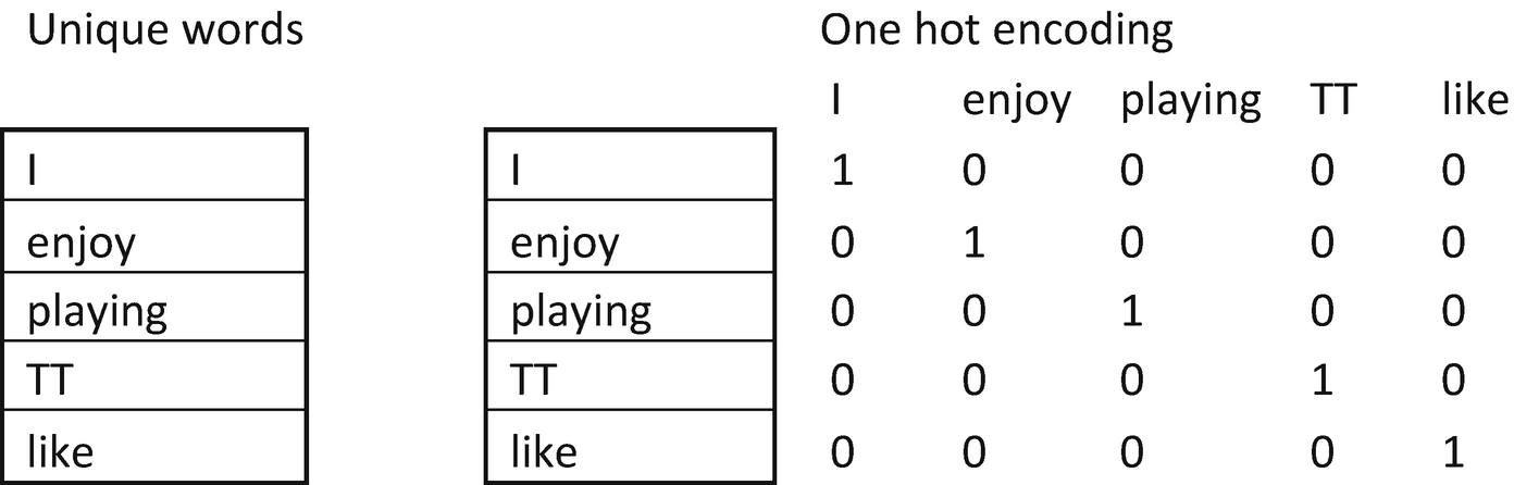
Notice that one-hot encoding results in each word being assigned a column. The major issue with one-hot-encoding is that the eucledian distance between the words {I, enjoy} is the same as the distance between the words {enjoy, like}. But we know that the distance between {I, enjoy} should be greater than the distance between {enjoy, like} because enjoy and like are more synonymous to each other.
Hand-Building a Word Vector
Before building a word vector, we’ll formulate the hypothesis as follows:
“Words that are related will have similar words surrounding them.”
For example, the words king and prince will have similar words surrounding them more often than not. Essentially, the context (the surrounding words) of the words would be similar.
By using the context words as input, we are trying to predict the given word as output.
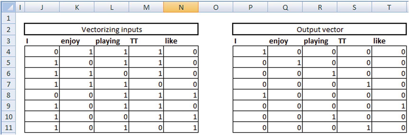
Note that, given the input words—{enjoy, playing, TT}—the vector form is {0,1,1,1,0} because the input doesn’t contain both I and like, so the first and last indices are 0 (note the one-hot encoding done in the first page).
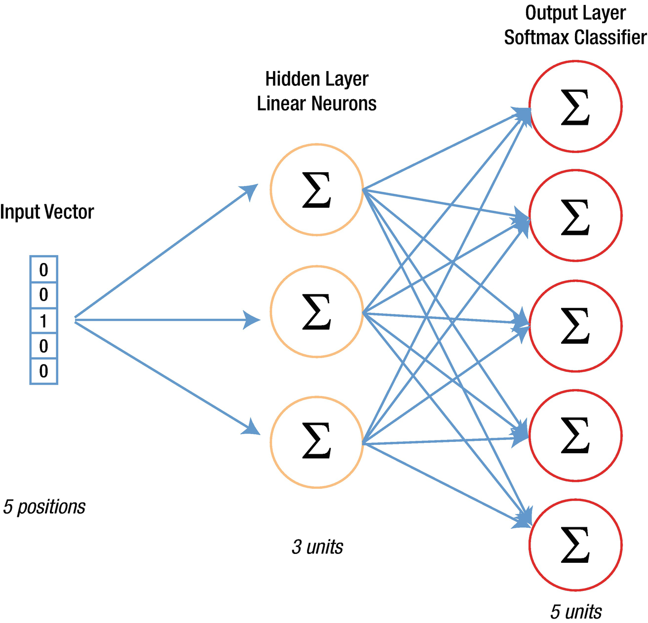
Our neural network
Layer | Size | Commentary |
|---|---|---|
Input layer | 8 × 5 | Because there are 8 inputs and 5 indices (unique words) |
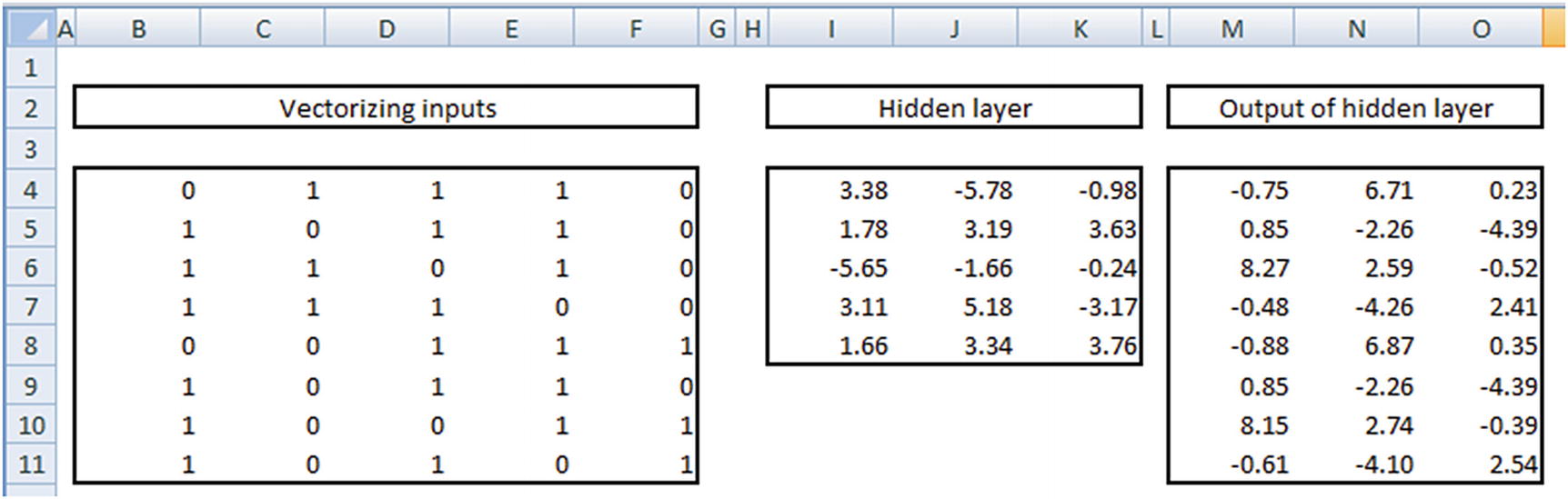
Weights at hidden layer | 5 × 3 | Because there are 5 inputs each to the 3 neurons |
Output of hidden layer | 8 × 3 | Matrix multiplication of input and hidden layer |
Weights from hidden to output | 3 × 5 | 3 output columns from hidden layer mapped to the 5 original output columns |
Output layer | 8 × 5 | Matrix multiplication between output of hidden layer and the weights from hidden to output layer |
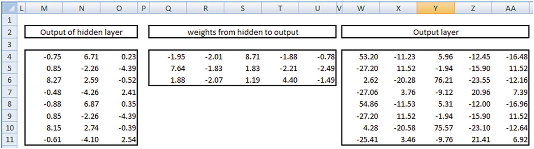
Once we have the output of the hidden layer, we multiply them with a matrix of weights from hidden to output layer. Given that the output of hidden layer is 8 × 3 in size and the hidden layer to output is 3 × 5 in size, our output layer is 8 × 5. But note that the output layer has a range of numbers, both positive and negative, as well as numbers that are >1 or <–1.
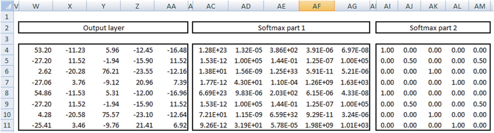
- 1.
Apply exponential to the number.
- 2.
Divide the output of step 1 by the row sum of the output of step 1.
In the preceding output, we see that the output of the first column is very close to 1 in the first row, and the output of the second column is 0.5 in the second row and so on.
Cross entropy loss = –∑ Actual value × Log (probability, 2)
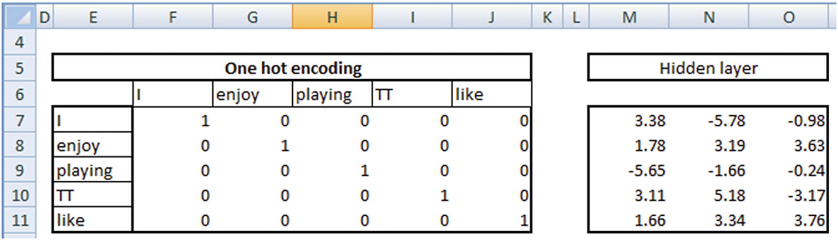
Now that we have the input words and the hidden layer weights calculated, the words can now be represented in a lower dimension by multiplying the input word with the hidden layer representation.
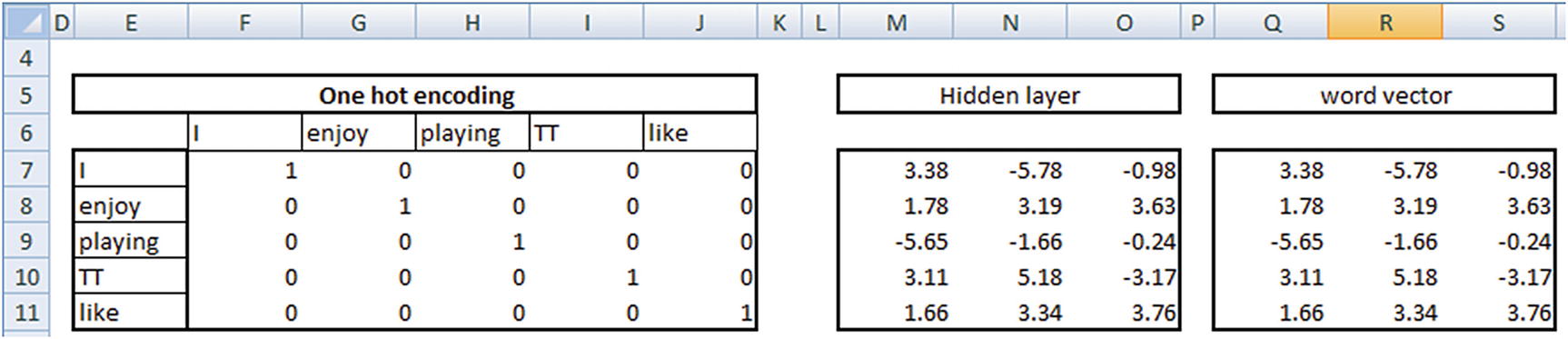
If we now consider the words {enjoy, like} we should notice that the vectors of the two words are very similar to each other (that is, the distance between the two words is small).
This way, we have converted the original input one-hot-encoded vector, where the distance between {enjoy, like} was high to the transformed word vector, where the distance between {enjoy, like} is small.
Methods of Building a Word Vector
The method we have adopted in building a word vector in the previous section is called the continuous bag of words (CBOW) model.
- 1.
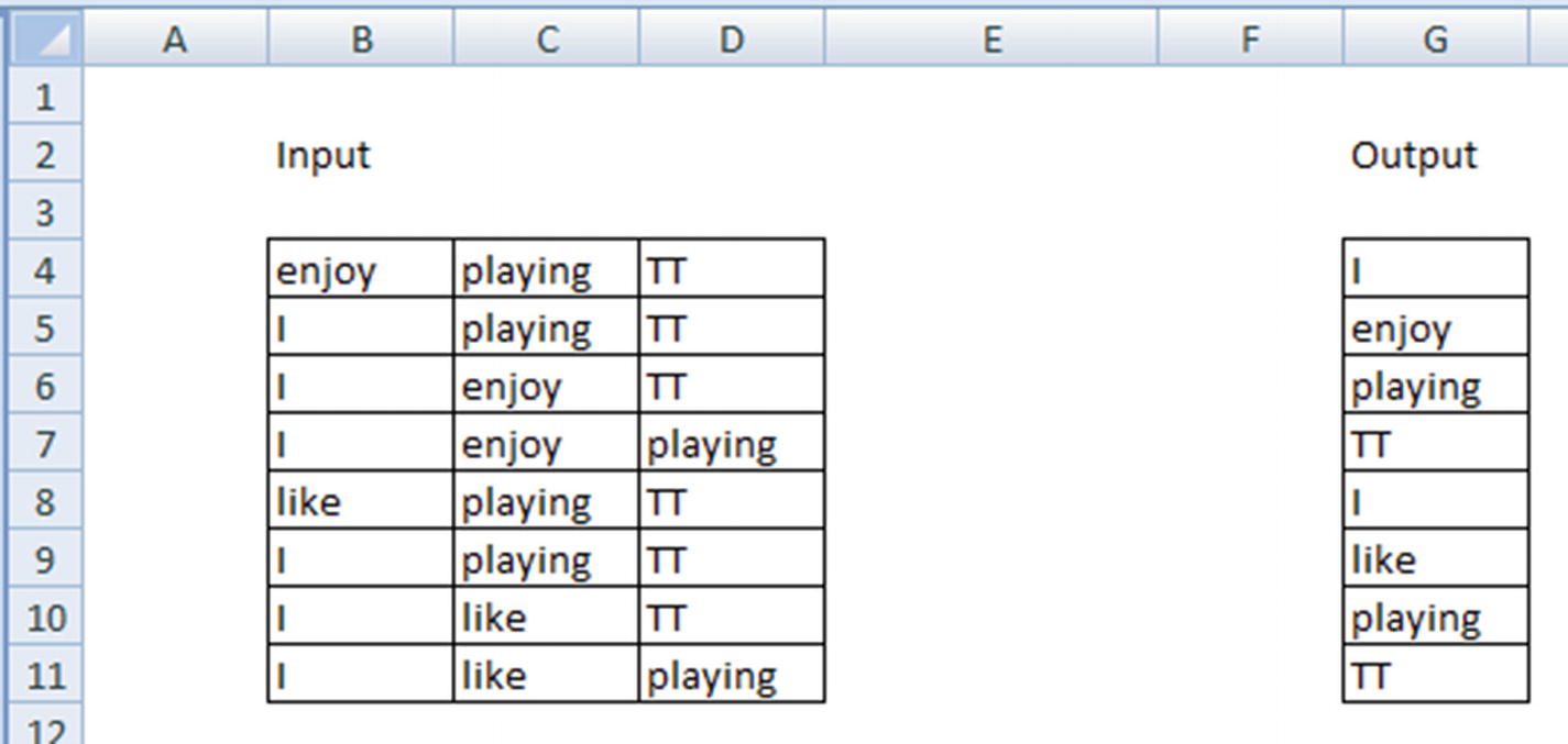
Fix a window size. That is, select n words to the left and right of a given word. For example, let’s say the window size is 2 words each to the left and right of the given word.
- 2.
Given the window size, the input and output vectors would look like this:
Input words | Output word |
|---|---|
{The, quick, fox, jumped} | {brown} |
{quick, brown, jumped, over} | {fox} |
{brown, fox, over, the} | {jumped} |
{fox, jumped, the, dog} | {over} |
Input words | Output word |
|---|---|
{brown} | {The, quick, fox, jumped} |
{fox} | {quick, brown, jumped, over} |
{jumped} | {brown, fox, over, the} |
{over} | {fox, jumped, the, dog} |
The approach to arrive at the hidden layer vectors remains the same, irrespective of whether it is a skip-gram model or a CBOW model.
Issues to Watch For in a Word2vec Model
For the way of calculation discussed so far, this section looks at some of the common issues we might be facing.
Frequent Words
Typical frequent words like the appear quite often in vocabulary. In such cases, the output has the words like the occurring a lot more often. If not treated, this might result in a majority of the output being the most frequent words, like the, more than other words. We need to have a way to penalize for the number of times a frequently occurring word can be seen in the training dataset.

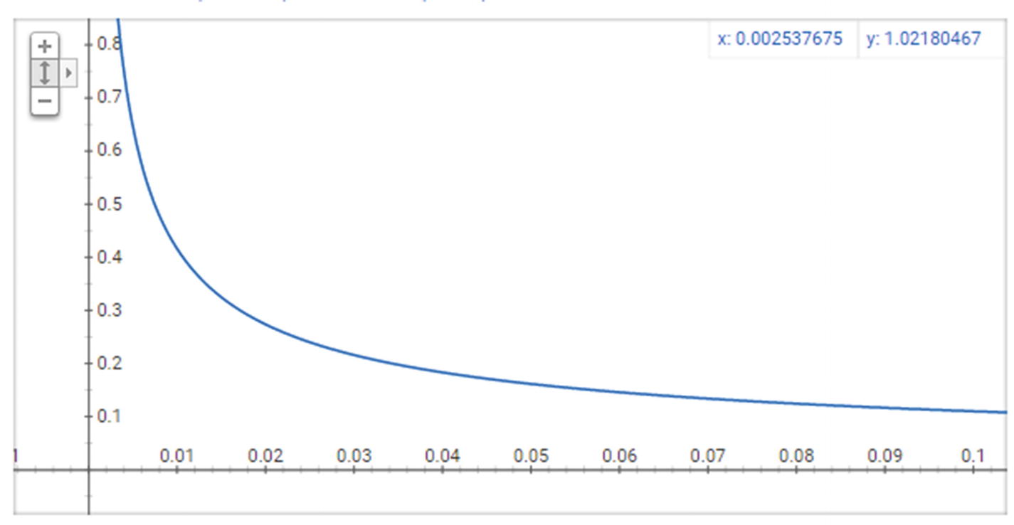
The resultant curve
Note that as z(w) (x-axis) increases, the probability of selection (y-axis) decreases drastically.
Negative Sampling
Let’s assume there are a total of 10,000 unique words in our dataset—that is, each vector is of 10,000 dimensions. Let’s also assume that we are creating a 300-dimensional vector from the original 10,000-dimensional vector. This means, from the hidden layer to the output layer, there are a total of 300 × 10,000 = 3,000,000 weights.
One of the major issues with such a high number of weights is that it might result in overfitting on top of the data. It also might result in a longer training time.
Negative sampling is one way to overcome this problem. Let’s say that instead of checking for all 10,000 dimensions, we pick the index at which the output is 1 (the correct label) and five random indices where the label is 0. This way, we are reducing the number of weights to be updated in a single iteration from 3 million to 300 × 6 = 1800 weights.
I said that the selection of negative indices is random, but in actual implementation of Word2vec, the selection is based on the frequency of a word when compared to the other words. The words that are more frequent have a higher chance of getting selected when compared to words that are less frequent.

Once the probabilities of each word are calculated, the word selection happens as follows: Higher-frequency words are repeated more often, and lower-frequent words are repeated less often and are stored in a table. Given that high-frequency words are repeated more often, the chance of them getting picked up is higher when a random selection of five words is made from the table.
Implementing Word2vec in Python
Word2vec can be implemented in Python using the gensim package (the Python implementation is available in github as “word2vec.ipynb”).
logging essentially helps us in tracking the extent to which the word vector calculation is complete.
num_features is the number of neurons in the hidden layer.
min_word_count is the cut-off of the frequency of words that get accepted for the calculation.
context is the window size
downsampling helps in assigning a lower probability of picking the more frequent words.
Note that all the input sentences are tokenized.
Once a model is trained, the vector of weights for any word in the vocabulary that meets the specified criterion can be obtained as follows:
Similarly, the most similar word to a given word can be obtained like this:
Summary
Word2vec is an approach that can help convert text words into numeric vectors.
This acts as a powerful first step for multiple approaches downstream—for example, one can use the word vectors in building a model.
Word2vec comes up with the vectors using one the CBOW or skip-gram model, which have a neural network architecture that helps in coming up with vectors.
The hidden layer in neural network is the key to generating the word vectors.