V Kishore AyyadevaraPro Machine Learning Algorithms https://doi.org/10.1007/978-1-4842-3564-5_7

7. Artificial Neural Network

V Kishore Ayyadevara¹

(1)

Hyderabad, Andhra Pradesh, India

Artificial neural network is a supervised learning algorithm that leverages a mix of multiple hyper-parameters that help in approximating complex relation between input and output. Some of the hyper-parameters in artificial neural network include the following:

Number of hidden layers
Number of hidden units
Activation function
Learning rate

In this chapter, you will learn the following:

Working details of neural networks
The impact of various hyper-parameters on neural networks
Feed-forward and back propagation
The impact of learning rate on weight updates
Ways to avoid Over-fitting in neural networks
How to implement neural network in Excel, Python, and R

Neural networks came about from the fact that not everything can be approximated by a linear/logistic regression—there may be potentially complex shapes within data that can only be approximated by complex functions. The more complex the function (with some way to take care of overfitting), the better is the accuracy of predictions. We’ll start by looking at how neural networks work toward fitting data into a model.

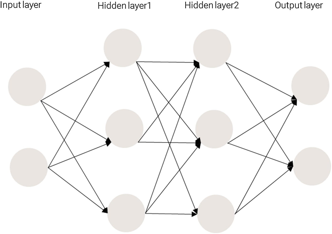
Structure of a Neural Network

The typical structure of a neural network is shown in Figure 7-1.

../images/463052_1_En_7_Chapter/463052_1_En_7_Fig1_HTML.jpg — Figure 7-1
Neural network structure

The input level/layer in the figure is typically the independent variables that are used to predict the output (dependent variable) level/layer. Typically in a regression problem, there will be only one node in output layer and in a classification problem, the output layer contains as many nodes as the number of classes (distinct values) present in dependent variable. The hidden level/layer is used to transform the input variables into a higher order function. The way the hidden layer transforms the output is shown in Figure 7-2.

../images/463052_1_En_7_Chapter/463052_1_En_7_Fig2_HTML.jpg — Figure 7-2
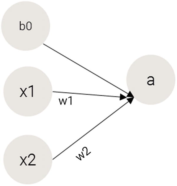
Transforming the output

In Figure 7.2, x1 and x2 are the independent variables, and b0 is the bias term (similar to the bias in linear/logistic regression). w1 and w2 are the weights given to each of the input variables. If a is one of the units/neurons in hidden layer, it is equal to the following:

$a=f\left(\sum \limits_{i=0}^N{w}_i{x}_i\right)$

The function in the preceding equation is the activation function we are applying on top of the summation so that we attain non-linearity (we need non-linearity so that our model can now learn complex patterns). The different activation functions are discussed in more detail in a later section.

Moreover, having more than one hidden layer helps in achieving high non-linearity. We want to achieve high non-linearity because without it, a neural network would be a giant linear function.

Hidden layers are necessary when the neural network has to make sense of something very complicated, contextual, or non-obvious, like image recognition. The term deep learning comes from having many hidden layers. These layers are known as hidden because they are not visible as a network output.

Working Details of Training a Neural Network

Training a neural network basically means calibrating all the weights by repeating two key steps: forward propagation and back propagation.

In forward propagation , we apply a set of weights to the input data and calculate an output. For the first forward propagation, the set of weights’ values are initialized randomly.

In back propagation , we measure the margin of error of the output and adjust the weights accordingly to decrease the error.

Neural networks repeat both forward and back propagation until the weights are calibrated to accurately predict an output.

Forward Propagation

Let’s go through a simple example of training a neural network to function as an exclusive or (XOR) operation to illustrate each step in the training process. The XOR function can be represented by the mapping of the inputs and outputs, as shown in the following table, which we’ll use as training data. It should provide a correct output given any input acceptable by the XOR function.

Input	Output
(0,0)	0
(0,1)	1
(1,0)	1
(1,1)	0

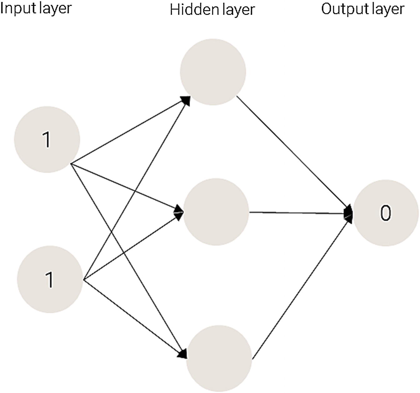
Let’s use the last row from the preceding table, (1,1) => 0, to demonstrate forward propagation, as shown in Figure 7-3. Note that, while this is a classification problem, we will still treat it as a regression problem, only to understand how forward and back propagation work.

../images/463052_1_En_7_Chapter/463052_1_En_7_Fig3_HTML.jpg — Figure 7-3
Applying a neural network

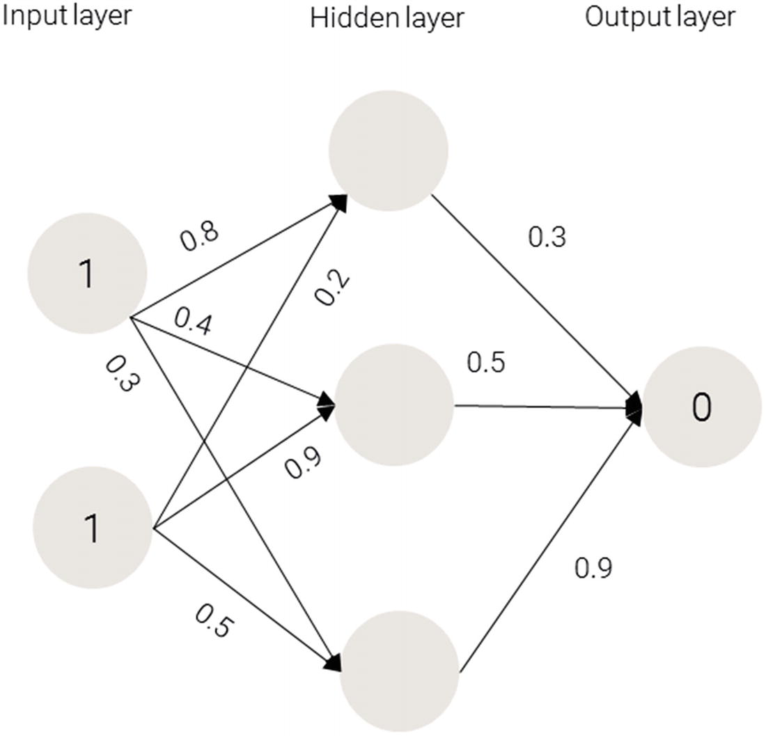
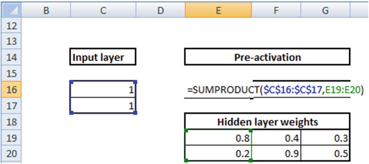
We now assign weights to all the synapses. Note that these weights are selected randomly (the most common way is based on Gaussian distribution) since it is the first time we’re forward propagating. The initial weights are randomly assigned to be between 0 and 1 (but note that the final weights don’t need to be between 0 and 1), as shown in Figure 7-4.

../images/463052_1_En_7_Chapter/463052_1_En_7_Fig4_HTML.jpg — Figure 7-4
Weights on the synapses

We sum the product of the inputs with their corresponding set of weights to arrive at the first values for the hidden layer (Figure 7-5). You can think of the weights as measures of influence that the input nodes have on the output:

1 × 0.8 + 1 × 0.2 = 1
1 × 0.4 + 1 × 0.9 = 1.3
1 × 0.3 + 1 × 0.5 = 0.8

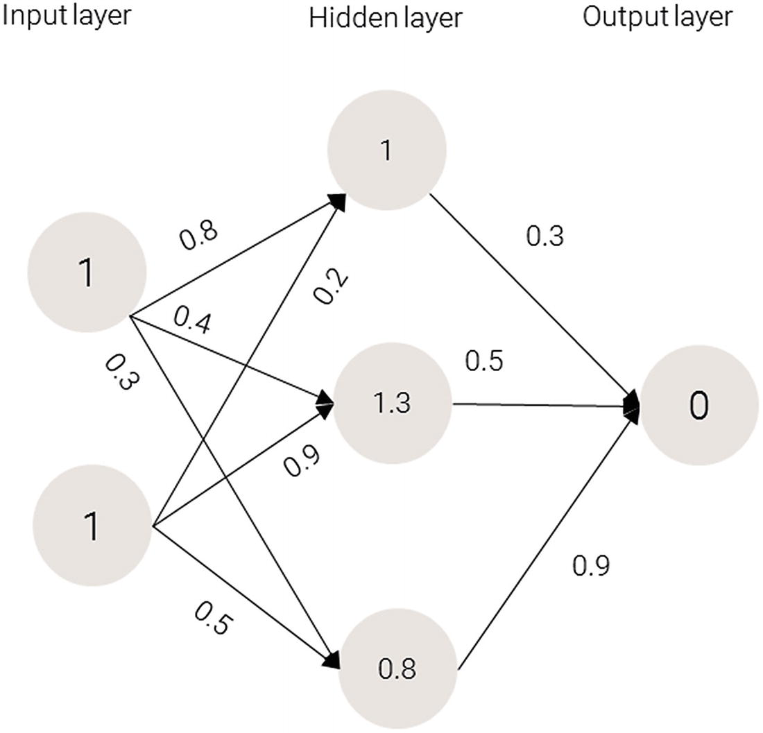
../images/463052_1_En_7_Chapter/463052_1_En_7_Fig5_HTML.jpg — Figure 7-5
Values for the hidden layer

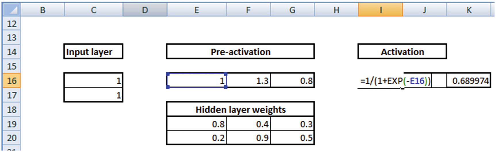
Applying the Activation Function

Activation functions are applied at the hidden layer of a neural network. The purpose of an activation function is to transform the input signal into an output signal. They are necessary for neural networks to model complex non-linear patterns that simpler models might miss.

Some of the major activation functions are as follows:

$\mathrm{Sigmoid}=1/\left(1+{e}^{-x}\right)$

$Tanh=\frac{e^x-{e}^{-x}}{e^x+{e}^{-x}}$

Rectified linear unit = x if x > 0, else 0

For our example, let’s use the sigmoid function for activation. And applying Sigmoid(x) to the three hidden layer sums, we get Figure 7-6:

Sigmoid(1.0) = 0.731
Sigmoid(1.3) = 0.785
Sigmoid(0.8) = 0.689

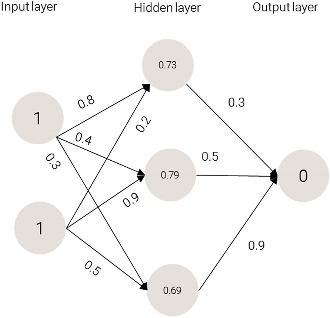
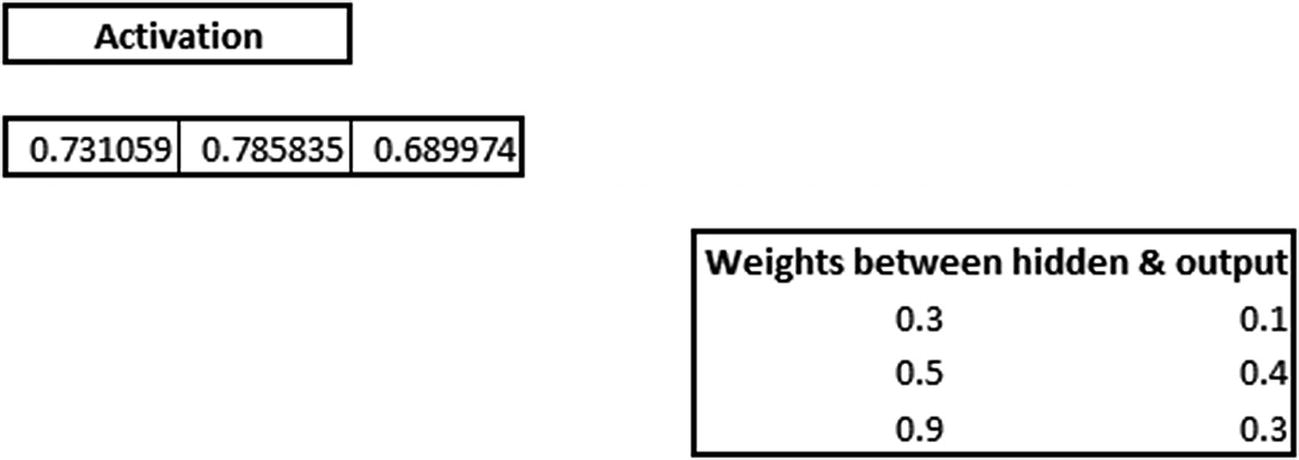
../images/463052_1_En_7_Chapter/463052_1_En_7_Fig6_HTML.jpg — Figure 7-6
Applying sigmoid to the hidden layer sums

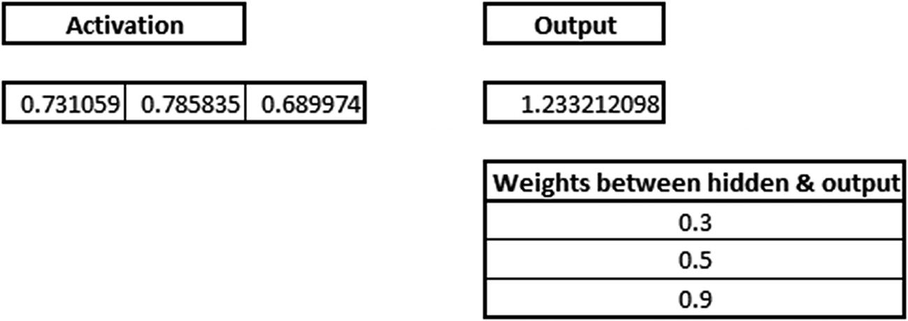
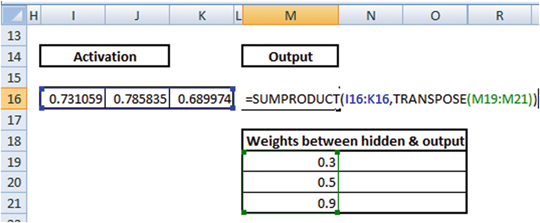
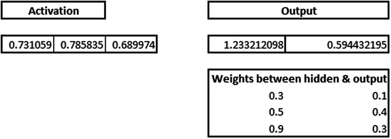
Then we sum the product of the hidden layer results with the second set of weights (also determined at random the first time around) to determine the output sum:

0.73 × 0.3 + 0.79 × 0.5 + 0.69 × 0.9 = 1.235

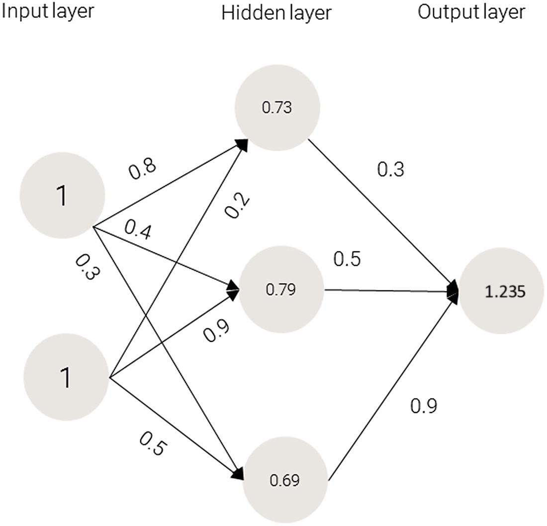
../images/463052_1_En_7_Chapter/463052_1_En_7_Fig7_HTML.jpg — Figure 7-7
Applying the activation function

Because we used a random set of initial weights, the value of the output neuron is off the mark—in this case, by 1.235 (since the target is 0).

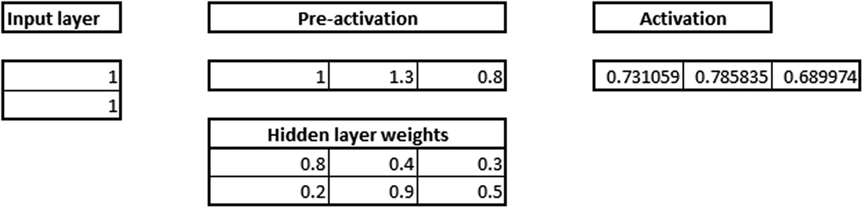
In Excel, the preceding would look as follows (the excel is available as “NN.xlsx” in github):

1.
The input layer has two inputs (1,1), thus input layer is of dimension of 1 × 2 (because every input has two different values).
2.
The 1 × 2 hidden layer is multiplied with a randomly initialized matrix of dimension 2 × 3.
3.
The output of input to hidden layer is a 1 × 3 matrix:

../images/463052_1_En_7_Chapter/463052_1_En_7_Figa_HTML.jpg

The formulas for the preceding outputs are as follows:

../images/463052_1_En_7_Chapter/463052_1_En_7_Figb_HTML.jpg

../images/463052_1_En_7_Chapter/463052_1_En_7_Figc_HTML.jpg

The output of the activation function is multiplied by a 3 × 1 dimensional randomly initialized matrix to get an output that is 1 × 1 in dimension:

../images/463052_1_En_7_Chapter/463052_1_En_7_Figd_HTML.jpg

The way to obtain the preceding output is per the following formula:

../images/463052_1_En_7_Chapter/463052_1_En_7_Fige_HTML.jpg

Again, while this is a classification exercise, where we use cross entropy error as loss function, we will still use squared error loss function only to make the back propagation calculations easier to understand. We will understand about how classification works in neural network in a later section.

Once we have the output, we calculate the squared error (Overall error) - which is (1.233-0)², as follows:

../images/463052_1_En_7_Chapter/463052_1_En_7_Figf_HTML.jpg

The various steps involved in obtaining squared error from an input layer, collectively form a forward propagation.

Back Propagation

In forward propagation, we took a step from input to hidden to output. In backward propagation , we take the reverse approach: essentially, change each weight starting from the last layer by a small amount until the minimum possible error is reached. When a weight is changed, the overall error either decreases or increases. Depending on whether error increased or decreased, the direction in which a weight is updated is decided. Moreover, in some scenarios, for a small change in weight, error increases/decreases by quite a bit, and in some cases error changes only by a small amount.

Summing it up, by updating weights by a small amount and measuring the change in error, we are able to do the following:

1.
Decide the direction in which weight needs to be updated
2.
Decide the magnitude by which the weights need to be updated

Before proceeding with implementing back propagation in Excel, let’s look at one additional aspect of neural networks: the learning rate . Learning rate helps us in building trust in our decision of weight updates. For example, while deciding on the magnitude of weight update, we would potentially not change everything in one go but rather take a more careful approach in updating the weights more slowly. This results in obtaining stability in our model. A later section discusses how learning rate helps in stability.

Working Out Back Propagation

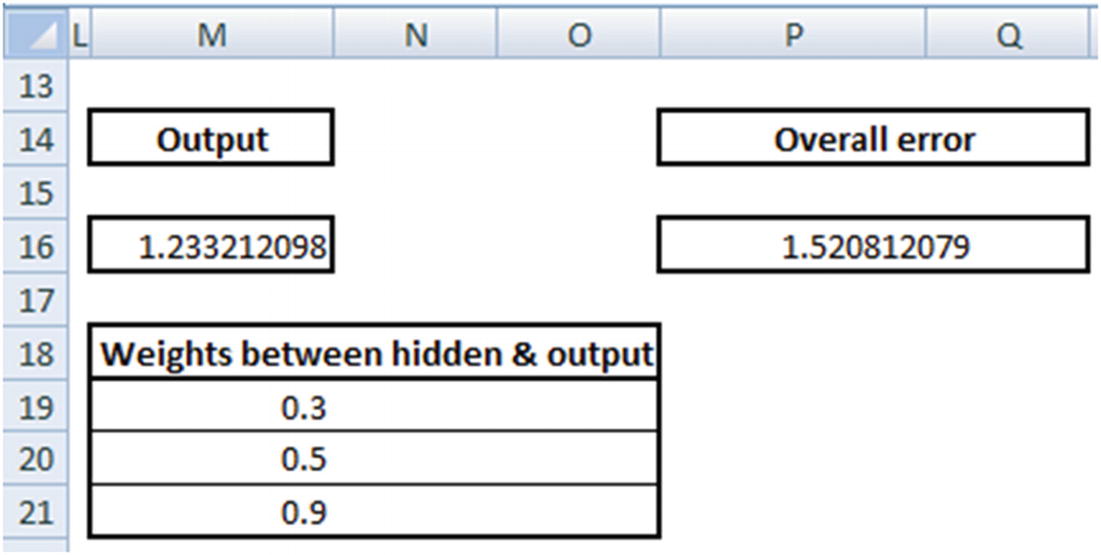
To see how back propagation works, let’s look at updating the randomly initialized weight values in the previous section.

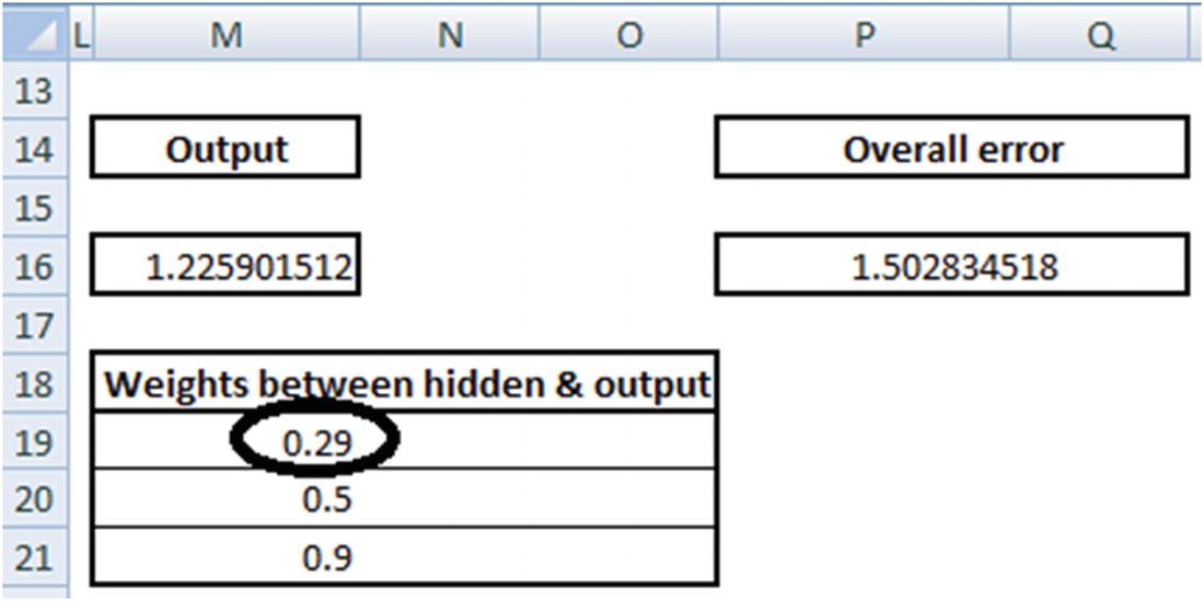
The overall error of the network with the randomly initialized weight values is 1.52. Let’s change the weight between hidden to output layer from 0.3 to 0.29 and see the impact on overall error:

../images/463052_1_En_7_Chapter/463052_1_En_7_Figg_HTML.jpg

Note that with a small decrease in weight, the overall error decreases from 1.52 to 1.50. Thus, from the two points mentioned earlier, we conclude that 0.3 needs to be reduced to a lower number. The question we need to answer after deciding the direction in which the weight needs to be updated is: “What is the magnitude of weight update?”

If error decreases by a lot from changing the weight by a small amount (0.01), then potentially, weights can be updated by a bigger amount. But if error decreases only by a small amount when weights get updated by a small amount, then weights need to be updated slowly. Thus the weight with a value of 0.3 between the hidden to output layer gets updated as follows:

0.3 – 0.05 × (Reduction in error because of change in weight)

The 0.05 there is the learning parameter, which is to be given as input by user - more on learning rate in the next section. Thus the weight value gets updated to 0.3 – 0.05 × ((1.52 - 1.50) / 0.01) = 0.21.

Similarly, the other weights get updated to 0.403 and 0.815:

../images/463052_1_En_7_Chapter/463052_1_En_7_Figh_HTML.jpg

Note that the overall error decreased by quite a bit by just changing the weights connecting the hidden layer to the output layer.

Now that we have updated the weights in one layer, we’ll update weights that exist in the earlier part of the network—that is, between input and hidden layer activation. Let’s change the weight values and calculate the change in error:

Original weight	Updated weight	Decrease in error
0.8	0.7957	0.0009
0.4	0.3930	0.0014
0.3	0.2820	0.0036
0.2	0.1957	0.0009
0.9	0.8930	0.0014
0.5	0.4820	0.0036

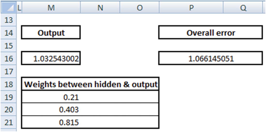
Given that error is decreasing every time when the weights are decreased by a small value, we will reduce all the weights to the value calculated above.

Now that the weights are updated, note that the overall error decreased from 1.52 to 1.05. We keep repeating the forward and backward propagation until the overall error is minimized as much as possible.

Stochastic Gradient Descent

Gradient descent is the way in which error is minimized in the scenario just discussed. Gradient stands for difference (the difference between actual and predicted) and descent means to reduce. Stochastic stands for the subset of training data considered to calculate error and thereby weight update (more on the subset of data in a later section).

Diving Deep into Gradient Descent

To further our understanding of gradient descent neural networks, let’s start with a known function and see how the weights could be derived: for now, we will have the known function as y = 6 + 5x.

The dataset would look as follows (available as “gradient descent batch size.xlsx” in github):

x	y
1	11
2	16
3	21
4	26
5	31
6	36
7	41
8	46
9	51
10	56

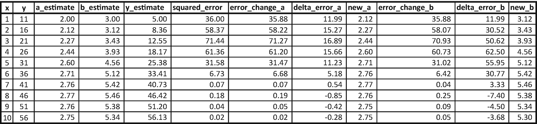
Let’s randomly initialize the parameters a and b to values of 2 and 3 (the ideal values of which are 5 and 6). The calculations of weight updates would be as follows:

../images/463052_1_En_7_Chapter/463052_1_En_7_Figx_HTML.png

Note that we started with the random initialization of a_estimate and b_estimate estimate with 2 and 3 (row 1, columns 3 and 4).

We calculate the following:

Calculate the estimate of y using the randomly initialized values of a and b: 5.
Calculate the squared error corresponding to the values of a and b (36 in row 1).
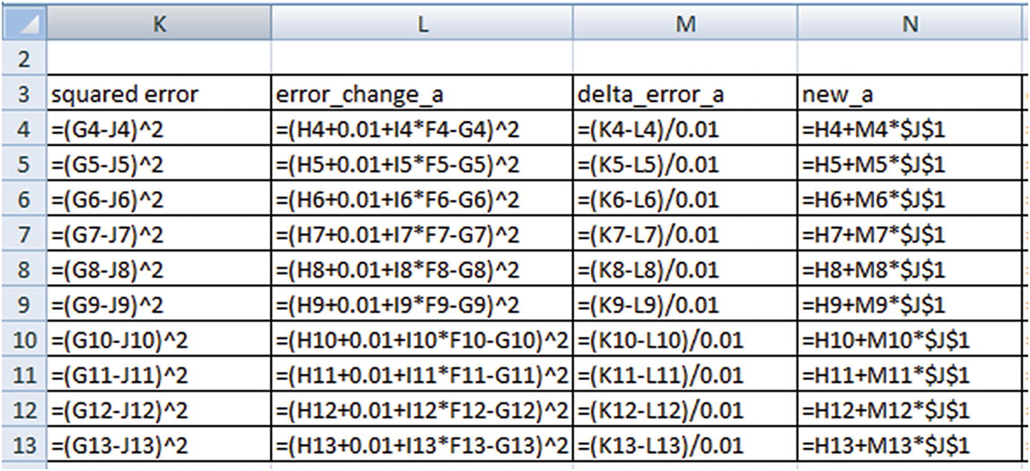
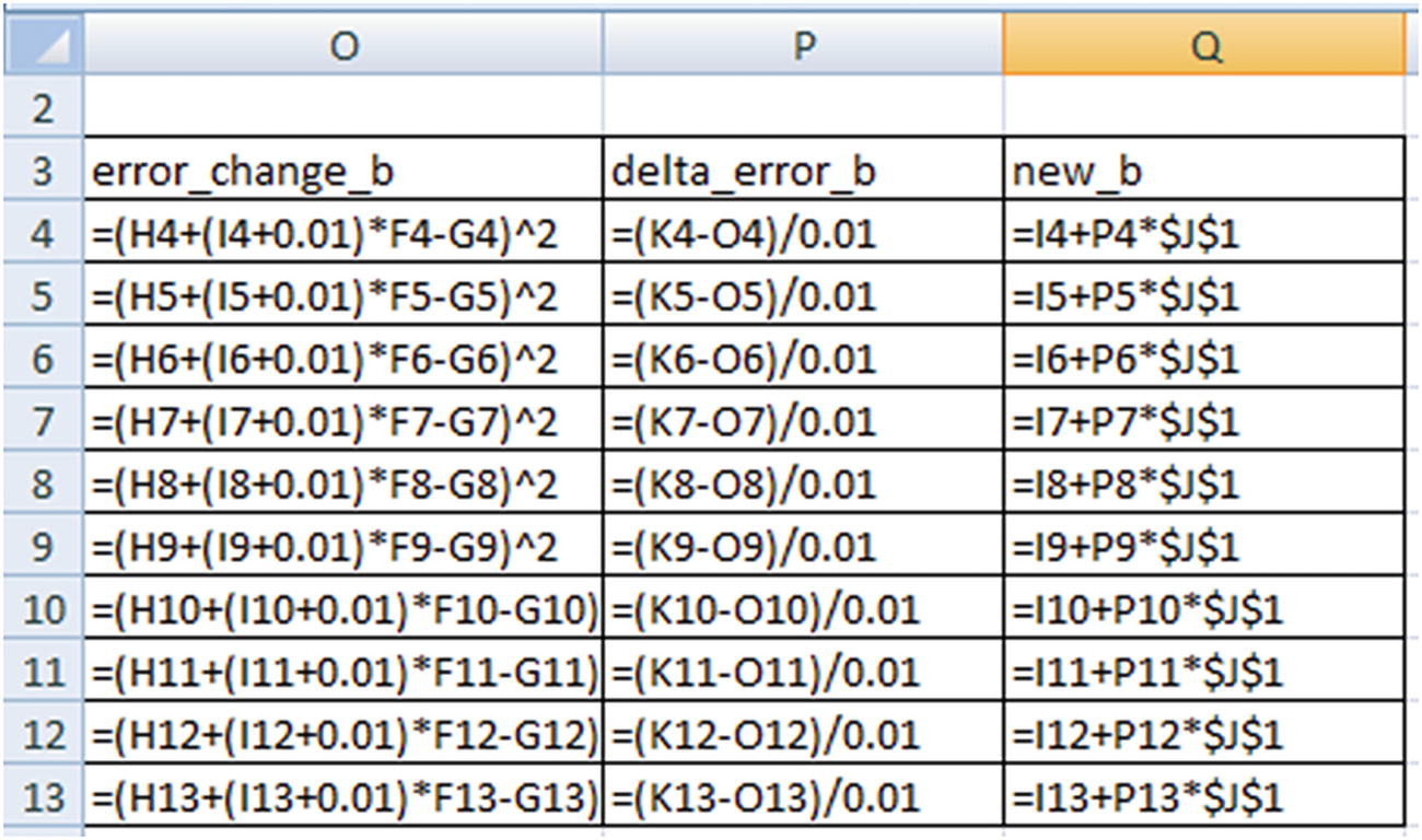
Change the value of a slightly (increase it by 0.01) and calculate the squared error corresponding to the changed a value. This is stored as the error_change_a column.
Calculate the change in error in delta_error_a (which is change in error / 0.01). Note that the delta would be very similar if we perform differentiation over loss function with respect to a.
Update the value of a based on: new_a = a_estimate + (delta_error_a) × learning_rate.

We consider the learning rate to be 0.01 in this analysis. Do the same analysis for the updated estimate of b. Here are the formulas corresponding to the calculations just described:

../images/463052_1_En_7_Chapter/463052_1_En_7_Figj_HTML.jpg

../images/463052_1_En_7_Chapter/463052_1_En_7_Figk_HTML.jpg

Once the values of a and b are updated (new_a and new_b are calculated in the first row), perform the same analysis on row 2 (Note that we start off row 2 with the updated values of a and b obtained from the previous row.) We keep on updating the values of a and b until all the data points are covered. At the end, the updated value of a and b are 2.75 and 5.3.

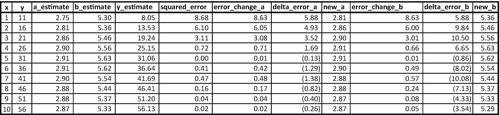
Now that we have run through the entire set of data, we’ll repeat the whole process with 2.75 and 5.3, as follows:

../images/463052_1_En_7_Chapter/463052_1_En_7_Figl_HTML.png

The values of a and b started at 2.75 and 5.3 and ended up at 2.87 and 5.29, which is a little more accurate than the previous iteration. With more iterations, the values of a and b would converge to the optimal value.

We’ve looked at the working details of basic gradient descent, but other optimizers perform a similar functionality. Some of them are as follows:

RMSprop
Adagrad
Adadelta
Adam
Adamax
Nadam

Why Have a Learning Rate?

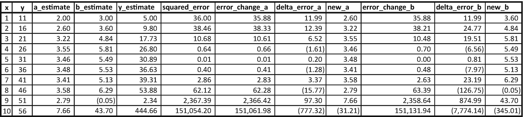
In the scenario just discussed, by having a learning rate of 0.01 we moved the weights from 2,3 to 2.75 and 5.3. Let’s look at how the weights would change had the learning rate been 0.05:

../images/463052_1_En_7_Chapter/463052_1_En_7_Figm_HTML.png

Note that the moment the learning rate changed from 0.01 to 0.05, in this particular case, the values of a and b started to have abnormal variations over the latter data points. Thus, a lower learning rate is always preferred. However, note that a lower learning rate would result in a longer time (more iterations) to get the optimal results.

Batch Training

So far, we have seen that the values of a and b get updated for every row of a dataset. However, that might not be a good idea, as variable values can significantly impact the values of a and b. Hence, the error calculation is typically done over a batch of data as follows. Let’s say the batch size is 2 (in the previous case, batch size was 1):

x	y	a_estimate	b_estimate	y_estimate	squared error	error_change_a	delta_error_a	new_a	error_change_b	delta_error_b	new_b
1	11	2	3	5	36	35.8801	11.99		35.8801	11.99
2	16	2	3	8	64	63.8401	15.99		63.6804	31.96
				Overall	100	99.7202	27.98	2.2798	99.5605	43.95	3.4395

Now for the next batch, the updated values of a and b are 2.28 and 3.44:

x	y	a_estimate	b_estimate	y_estimate	squared error	error_change_a	delta_error_a	new_a	error_change_b	delta_error_b	new_b
3	21	2.28	3.44	12.60	70.59	70.42	16.79		70.09	50.32
4	26	2.28	3.44	16.04	99.25	99.05	19.91		98.45	79.54
				Overall	169.83	169.47	36.71	2.65	168.54	129.86	4.74

The updated values of a and b are now 2.65 and 4.74, and the iterations continue. Note that, in practice, batch size is at least 32.

The Concept of Softmax

So far, in the Excel implementations, we have performed regression and not classification. They key difference to note when we perform classification is that the output is bound between 0 and 1. In the case of a binary classification, the output layer would have two nodes instead of one. One node corresponds to an output of 0, and the other corresponds to an output of 1.

Now we’ll look at how our calculation changes for the discussion in the previous section (where the input is 1,1 and the expected output is 0) when the output layer has two nodes. Given that the output is 0, we will one-hot-encode the output as follows: [1,0], where the first index corresponds to an output of 0 and the second index value corresponds to an output of 1.

The weight matrix connecting the hidden layer and the output layer gets changed as follows: instead of a 3 × 1 matrix, it becomes a 3 × 2 matrix, because the hidden layer is now connected to two output nodes (unlike the regression exercise, where it was connected to 1 node):

../images/463052_1_En_7_Chapter/463052_1_En_7_Fign_HTML.jpg

Note that because the output nodes are to, our output layer also contains two values, as follows:

../images/463052_1_En_7_Chapter/463052_1_En_7_Figo_HTML.jpg

The one issue with the preceding output is that it has values that are >1 (in other cases, the values could be <0 as well).

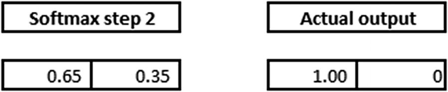
Softmax activation comes in handy in such scenario, where the output is beyond the expected value between 0 and 1. Softmax of the above output is calculated as follows:

In Softmax step 1 below, the output is raised to its exponential value. Note that 3.43 is the exponential of 1.233:

../images/463052_1_En_7_Chapter/463052_1_En_7_Figp_HTML.jpg

In Softmax step 2 below, the softmax output is normalized to get the probabilities in such a way that the sum of probability of both outputs is 1:

../images/463052_1_En_7_Chapter/463052_1_En_7_Figq_HTML.jpg

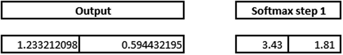
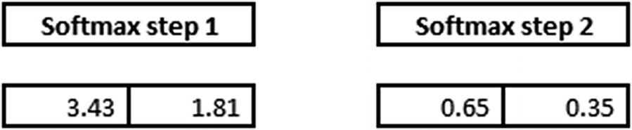
Note that the value of 0.65 is obtained by 3.43 / (3.43 + 1.81).

Now that we have the probability values, instead of calculating the overall squared error, we calculate the cross entropy error, as follows:

1.
The final softmax step is compared with actual output:
2.
The cross entropy error is calculated based on the actual values and the predicted values (which are obtained from softmax step 2):

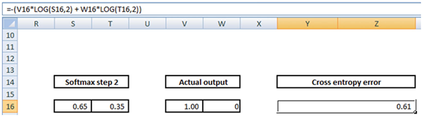
Note the formula for cross entropy error in the formula pane.

Now that we have the final error measure, we deploy gradient descent again to minimize the overall cross entropy error.

Different Loss Optimization Functions

One can optimize for different measures—for example, squared error in regression and cross entropy error in classification. The other loss functions that can be optimized include the following:

Mean squared error
Mean absolute percentage error
Mean squared logarithmic error
Squared hinge
Hinge
Categorical hinge
Logcosh
Categorical cross entropy
Sparse categorical cross entropy
Binary cross entropy
Kullback Leibler divergence
Poisson
Cosine proximity

Scaling a Dataset

Typically, neural networks perform well when we scale the input datasets. In this section, we’ll look at the reason for scaling. To see the impact of scaling on outputs, we’ll contrast two scenarios .

Scenario Without Scaling the Input

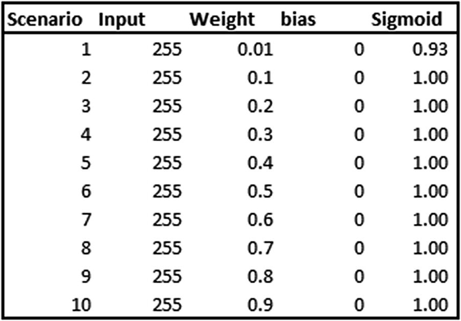
../images/463052_1_En_7_Chapter/463052_1_En_7_Figt_HTML.jpg

In the preceding table, various scenarios are calculated where the input is always the same, 255, but the weight that multiplies the input is different in each scenario. Note that the sigmoid output does not change, even though the weight varies by a lot. That’s because the weight is multiplied by a large number, the output of which is also a large number.

Scenario with Input Scaling

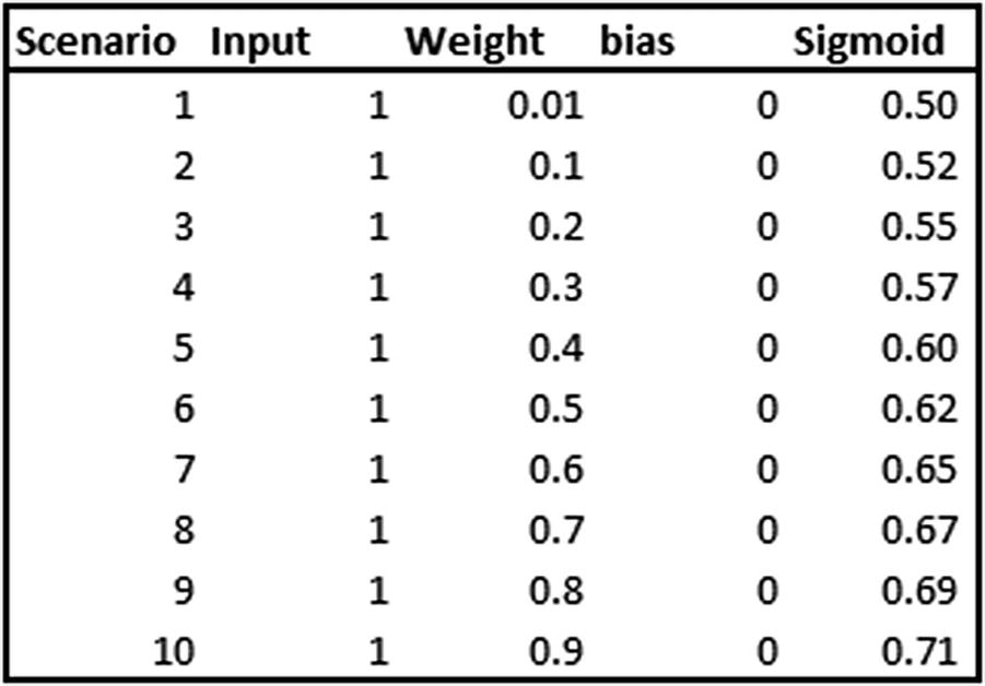
In this scenario, we’ll multiply different weight values by a small input number, as follows:

../images/463052_1_En_7_Chapter/463052_1_En_7_Figu_HTML.jpg

Now that weights are multiplied by a smaller number, sigmoid output differs by quite a bit for differing weight values.

The problem with a high magnitude of independent variables is significant as the weights need to be adjusted slowly to arrive at the optimal weight value. Given that the weights get adjusted slowly (per the learning rate in gradient descent), it may take considerable time to arrive at the optimal weights when the input is a high magnitude number. Thus, to arrive at an optimal weight value, it is always better to scale the dataset first so that we have our inputs as a small number.

Implementing Neural Network in Python

There are several ways of implementing neural network in Python. Here, we’ll look at implementing neural network using the keras framework . You must install tensorflow/ theano, and keras before you can implement neural network.

1.
Download the dataset and extract the train and test dataset (code available as “NN.ipynb” in github)

from keras.datasets import mnist
import matplotlib.pyplot as plt
%matplotlib inline
# load (downloaded if needed) the MNIST dataset
(X_train, y_train), (X_test, y_test) = mnist.load_data()
# plot 4 images as gray scale
plt.subplot(221)
plt.imshow(X_train[0], cmap=plt.get_cmap('gray'))
plt.subplot(222)
plt.imshow(X_train[1], cmap=plt.get_cmap('gray'))
plt.subplot(223)
plt.imshow(X_train[2], cmap=plt.get_cmap('gray'))
plt.subplot(224)
plt.imshow(X_train[3], cmap=plt.get_cmap('gray'))
# show the plot
plt.show()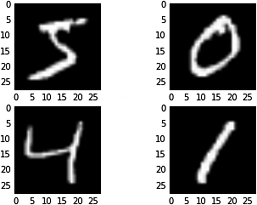

Figure 7-8
The output
2.
Import the relevant packages:

import numpy as np
from keras.datasets import mnist
from keras.models import Sequential
from keras.layers import Dense
from keras.layers import Dropout
from keras.utils import np_utils
3.
Pre-process the dataset:

num_pixels = X_train.shape[1] * X_train.shape[2]
# reshape the inputs so that they can be passed to the vanilla NN
X_train = X_train.reshape(X_train.shape[0],num_pixels ).astype('float32')
X_test = X_test.reshape(X_test.shape[0],num_pixels).astype('float32')
# scale inputs
X_train = X_train / 255
X_test = X_test / 255
# one hot encode the output
y_train = np_utils.to_categorical(y_train)
y_test = np_utils.to_categorical(y_test)
num_classes = y_test.shape[1]
4.
Build a model:

# building the model
model = Sequential()
# add 1000 units in the hidden layer
# apply relu activation in hidden layer
model.add(Dense(1000, input_dim=num_pixels,activation='relu'))
# initialize the output layer
model.add(Dense(num_classes, activation="softmax"))
# compile the model
model.compile(loss='categorical_crossentropy', optimizer="adam", metrics=['accuracy'])
# extract the summary of model
model.summary()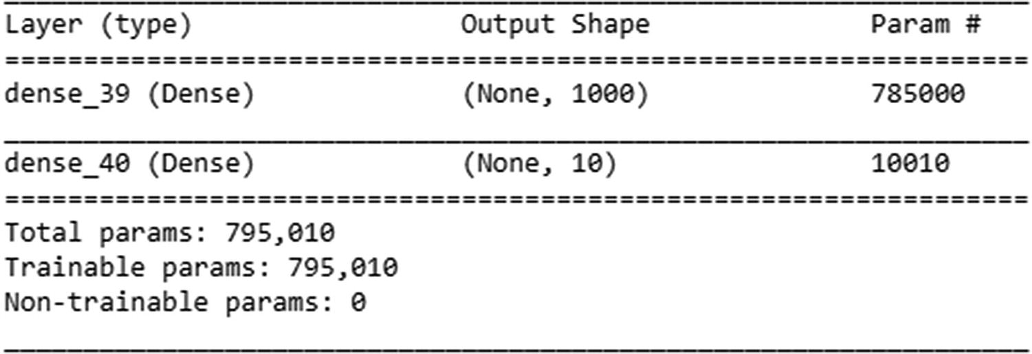
5.
Run the model:

model.fit(X_train, y_train, validation_data=(X_test, y_test), epochs=5, batch_size=1024, verbose=1)

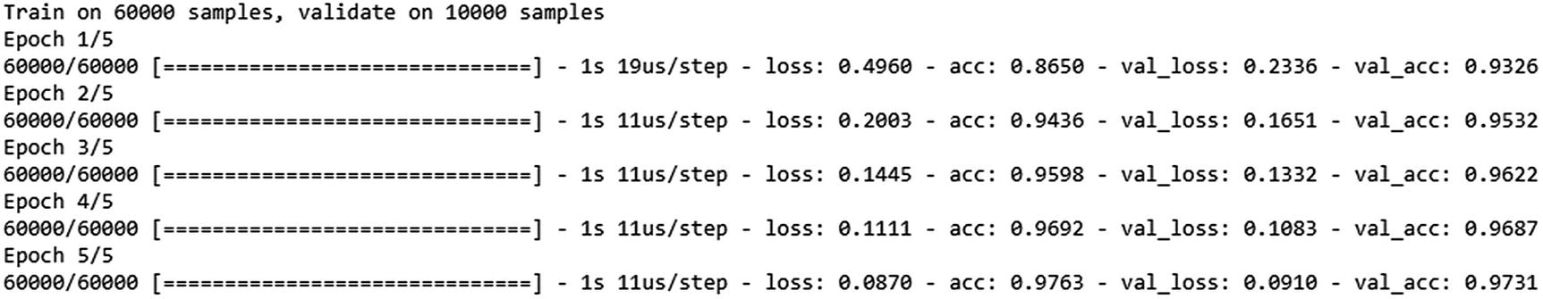
../images/463052_1_En_7_Chapter/463052_1_En_7_Figw_HTML.jpg

Note that as the number of epochs increases, accuracy on the test dataset increases as well. Also, in keras we only need to specify the input dimensions in the first layer, and it automatically figures the dimensions for the rest of the layers.

Avoiding Over-fitting using Regularization

Even though we have scaled the dataset, neural networks are likely to overfit on training dataset, as, the loss function (squared error or cross entropy error) ensures that loss is minimized over increasing number of epochs.

However, while training loss keeps on decreasing, it is not necessary that loss on test dataset is also decreasing. With more number of weights (parameters) in a neural network, the chances of over-fitting on training dataset and thus not generalizing on an unseen test dataset is high.

Let us contrast two scenario using the same neural network architecture on MNIST dataset, where in scenario A we consider 5 epochs and thus less chances of over-fitting, while in scenario B, we consider 100 epochs and thus more chances of over-fitting (code available as “Need for regularization in neural network.ipynb” in github).

We should notice that the difference between training and test dataset accuracy is less in the initial few epochs, but as the number of epochs increase, accuracy on training dataset increases, while the test dataset accuracy might not increase after some epochs.

In the case of our run, we see the following accuracy metrics:

Scenario	Training dataset	Test dataset
5 epochs	97.57%	97.27%
100 epochs	100%	98.28%

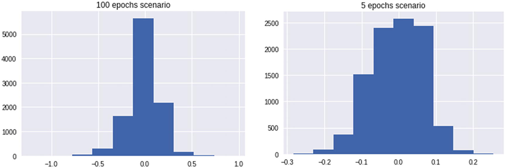
Once we plot the histogram of weights (for this example, the weights connecting hidden layer to output layer), we will notice that weights have a higher spread (range) in 100 epochs scenario, when compared to weights in 5 epochs scenario, as shown in the below picture:

../images/463052_1_En_7_Chapter/463052_1_En_7_Figy_HTML.jpg

100 epochs scenario had higher weight range, as it was trying to adjust for the edge cases in training dataset over the later epochs, while 5 epochs scenario did not have the opportunity to adjust for the edge cases. While training dataset’s edge cases got covered by the weight updates, it is not necessary that test dataset edge cases behave similarly and thus might not have got covered by weight updates. Also, note that an edge case in training dataset can be covered by giving a very high weightage to certain pixels and thus moving quickly towards saturating to either 1 or 0 of the sigmoid curve.

Thus, having high weight values are not desirable for generalization purposes. Regularization comes in handy in such scenario.

Regularization penalizes for having high magnitude of weights. The major types of regularization used are - L1 & L2 regularization

L2 regularization adds the additional cost term to error (loss function) as $\sum {w}_i^2$

L1 regularization adds the additional cost term to error (loss function) as $\sum \mid {w}_i\mid$

This way, we make sure that weights cannot be adjusted to have a high value so that they work for extreme edge cases in only train dataset.

Assigning Weightage to Regularization term

We notice that our modified loss function, in case of L2 regularization is as follows:

Overall Loss = $\sum {\left(y-\widehat{y}\right)}^2+\lambda \sum {w}_i^2$

where $\lambda$ is the weightage associated with the regularization term and is a hyper-parameter that needs to be tuned. Similarly, overall loss in case of L1 regularization is as follows:

Overall Loss = $\sum {\left(y-\widehat{y}\right)}^2+\lambda \sum \mid {w}_i\mid$

L1/ L2 regularization is implemented in Python as follows:

from keras import regularizers

model3 = Sequential()

model3.add(Dense(1000, input_dim=784, activation="relu", kernel_regularizer=regularizers.l2(0.001)))

model3.add(Dense(10, activation="softmax", kernel_regularizer=regularizers.l2(0.001)))

model3.compile(loss='categorical_crossentropy', optimizer="adam", metrics=['accuracy'])

model3.fit(X_train, y_train, validation_data=(X_test, y_test), epochs=100, batch_size=1024, verbose=2)

Notice that, the above involves, invoking an additional hyper-parameter - “kernel_regularizer” and then specifying whether it is an L1 / L2 regularization. Further we also specify the $\lambda$ value that gives the weightage to regularization.

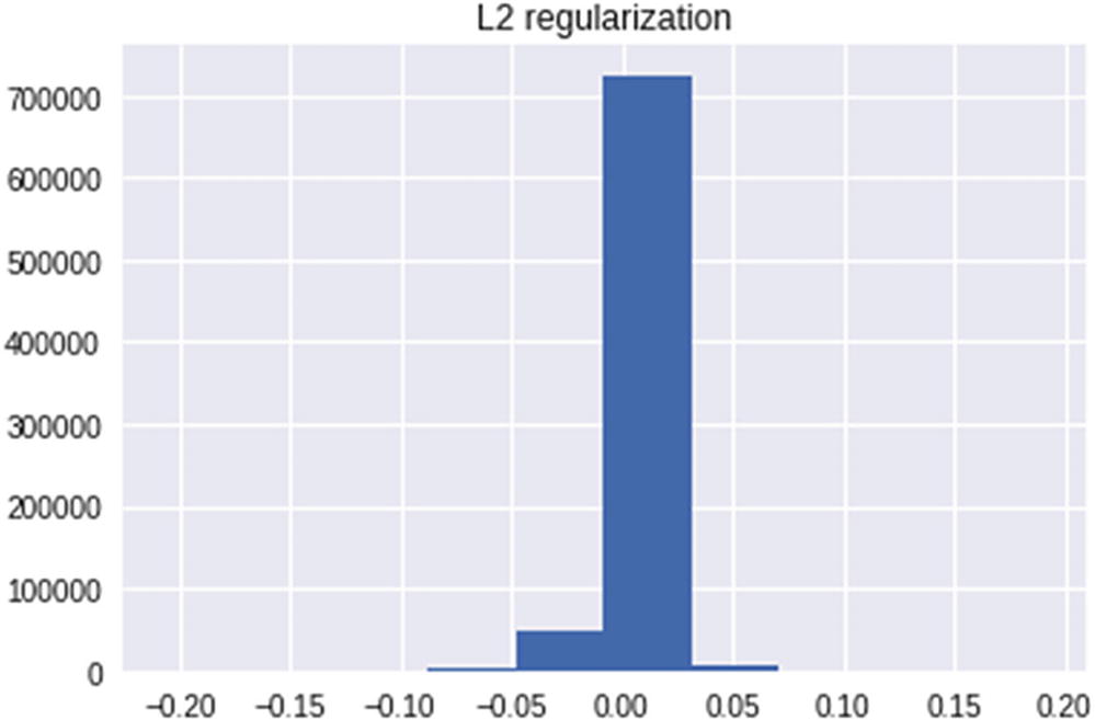
We notice that, post regularization, training and test dataset accuracy are similar to each other, where training dataset accuracy is 97.6% while test dataset accuracy is 97.5%. The histogram of weights post L2 regularization is as follows:

../images/463052_1_En_7_Chapter/463052_1_En_7_Figz_HTML.jpg

We notice that a majority of weights are now much closer to 0 when compared to the previous two scenarios and thus avoiding the overfitting issue that was caused due to high weight values assigned for edge cases. We would see a similar trend in case of L1 regularization.

Thus, L1 and L2 regularizations help us in avoiding the issue of overfitting on top of training dataset but not generalizing on test dataset.

Implementing Neural Network in R

Similar to the way we implemented a neural network in Python, we will use the keras framework to implement neural network in R . As with Python, multiple packages help us achieve the result.

In order to build neural network models, we will use the kerasR package in R. Given all the dependencies that the kerasR package has on Python, and the need to create a virtual environment, we will perform R implementation in the cloud, as follows (code available as “NN.R” in github):

1.
Install the kerasR package:

install.packages("kerasR")
2.
Load the installed package :

library(kerasR)
3.
Use the MNIST dataset for analysis:

mnist <- load_mnist()
4.
Examine the structure of the mnist object:

str(mnist)

Note that by default the MNIST dataset has the train and test datasets split.
5.
Extract the train and test datasets:

mnist <- load_mnist()
X_train <- mnist$X_train
Y_train <- mnist$Y_train
X_test <- mnist$X_test
Y_test <- mnist$Y_test
6.
Reshape the dataset.
Given that we are performing a normal neural network operation, our input dataset should be of the dimensions (60000,784), whereas X_train is of the dimension (60000,28,28):

X_train <- array(X_train, dim = c(dim(X_train)[1], 784))
X_test <- array(X_test, dim = c(dim(X_test)[1], 784))
7.
Scale the datasets:

X_train <- X_train/255
X_test <- X_test/255
8.
Convert the dependent variables (Y_train and Y_test) into categorical variables:

Y_train <- to_categorical(mnist$Y_train, 10)
Y_test <- to_categorical(mnist$Y_test, 10)
9.
Build a model :

model <- Sequential()
model$add(Dense(units = 1000, input_shape = dim(X_train)[2],activation = "relu"))
model$add(Dense(10,activation = "softmax"))
model$summary()
10.
Compile the model:

keras_compile(model, loss = 'categorical_crossentropy', optimizer = Adam(),metrics='categorical_accuracy')
11.
Fit the model:

keras_fit(model, X_train, Y_train,batch_size = 1024, epochs = 5,verbose = 1, validation_data = list(X_test,Y_test))

The process we just went through should give us a test dataset accuracy of ~98%.

Summary

In this chapter, you learned the following:

Neural network can approximate complex functions (because of the activation in hidden layers)
A forward and a backward propagation constitute the building blocks of the functioning of a neural network
Forward propagation helps us in estimating the error, whereas backward propagation helps in reducing the error
It is always a better idea to scale the input dataset whenever gradient descent is involved in arriving at the optimal weight values
L1/ L2 regularization helps in avoiding over-fitting by penalizing for high weight magnitudes

Previous Chapter

6. Gradient Boosting Machine

Next Chapter

8. Word2vec

Table of Contents for Pro Machine Learning Algorithms : A Hands-On Approach to Implementing Algorithms in Python and R