In Chapter 4, we looked at the process of building a decision tree. Decision trees can overfit on top of the data in some cases—for example, when there are outliers in dependent variable. Having correlated independent variables may also result in the incorrect variable being selected for splitting the root node.
Random forest overcomes those challenges by building multiple decision trees, where each decision tree works on a sample of the data. Let’s break down the term: random refers to the random sampling of data from original dataset, and forest refers to the building of multiple decision trees, one each for each random sample of data. (Get it? It is a combination of multiple trees, and so is called a forest.)
Working details of random forest
Advantages of random forest over decision tree
The impact of various hyper-parameters on a decision tree
How to implement random forest in Python and R
A Random Forest Scenario
- 1.You ask for recommendations from a person A.
- a.A asks some questions to find out what your preferences are.
- i.
We’ll assume only 20 exhaustive questions are available.
- ii.
We’ll add the constraint that any person can ask from a random selection of 10 questions out of the 20 questions.
- iii.
Given the 10 questions, the person ideally orders those questions in such a way that they are in a position to extract the maximum information from you.
- i.
- b.
Based on your responses, A comes up with a set of recommendations for movies.
- a.
- 2.You ask for recommendations from another person, B.
- a.As before, B asks questions to find out your preferences.
- i.
B is also in a position to ask only 10 questions out of the exhaustive list of 20 questions.
- ii.
Based on the set of 10 randomly selected questions, B again orders them to maximize the information obtained from your preferences.
- iii.
Note that the set of questions is likely to be different between A and B, though with some overlap.
- i.
- b.
Based on your responses, B comes up with recommendations.
- a.
- 3.In order to achieve some randomness, you may have told A that The Godfather is the best movie you have ever watched. But you merely told B you enjoyed watching The Godfather “a lot.”
- a.
This way, although the original information did not change, the way in which the two different people learned it was different.
- a.
- 4.You perform the same experiment with n friends of yours.
- a.
Through the preceding, you have essentially built an ensemble of decision trees (where ensemble means combination of trees or forest).
- a.
- 5.
The final recommendation will be the average recommendation of all n friends.
Bagging
Bagging is short for bootstrap aggregating . The term bootstrap refers to selecting a few rows randomly (a sample from the original dataset), and aggregating means taking the average of predictions from all the decision trees that are built on the sample of the dataset.
This way, the predictions are less likely to be biased due to a few outlier cases (because there could be some trees built using sample data—where the sample data did not have any outliers). Random forest adopts the bagging approach in building predictions.
Working Details of a Random Forest
- 1.
Subset the original data so that the decision tree is built on only a sample of the original dataset.
- 2.
Subset the independent variables (features) too while building the decision tree.
- 3.
Build a decision tree based on the subset data where the subset of rows as well as columns is used as the dataset.
- 4.
Predict on the test or validation dataset.
- 5.
Repeat steps 1 through 3 n number of times, where n is the number of trees built.
- 6.
The final prediction on the test dataset is the average of predictions of all n trees.
The following code in R builds the preceding algorithm (available as “rf_code.R” in github):
The described dataset has 140 columns and 10,000 rows. The first 8,000 rows are used to train the model, and the rest are used for testing:
Given that we are using decision trees to build our random forest, let’s use the rpart package:
Implementing a Random Forest in R
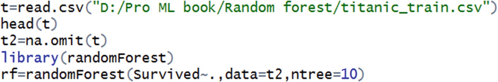
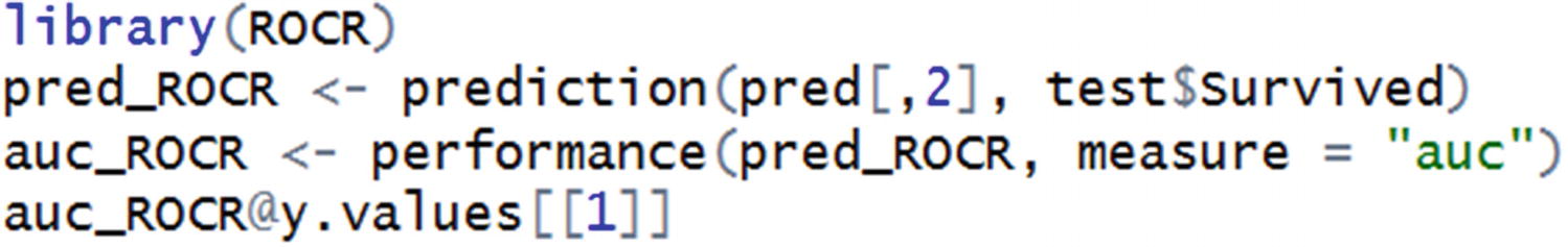
Random forest can be implemented in R using the randomForest package. In the following code snippet, we try predicting whether a person would survive or not in the Titanic dataset (the code is available as “rf_code2.R” in github).
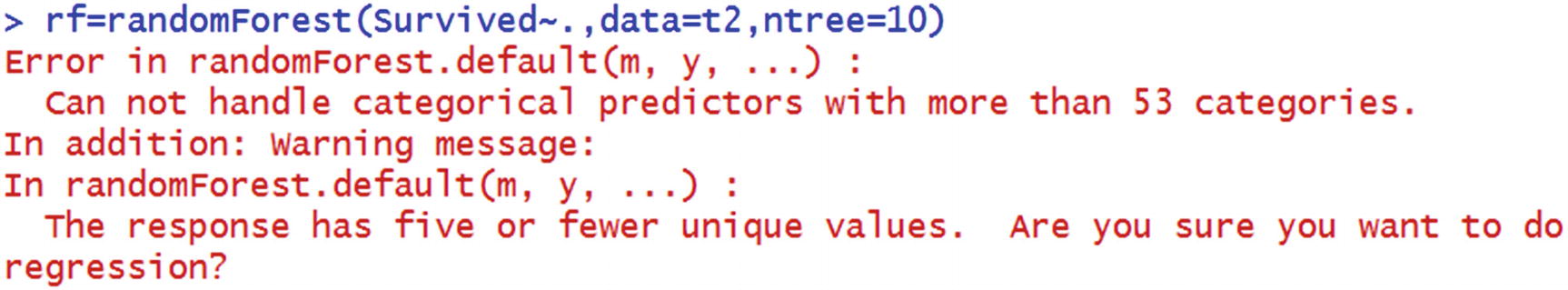
The number of distinct values in some categorical independent variables is high.
Additionally, it assumes that we would have to specify regression instead of classification.
Let’s look at why random forest might have given an error when the categorical variable had a high number of distinct values. Note that random forest is an implementation of multiple decision trees. In a decision tree, when there are more distinct values, the frequency count of a majority of the distinct values is very low. When frequency is low, the purity of the distinct value is likely to be high (or impurity is low). But this isn’t reliable, because the number of data points is likely to be low (in a scenario where the number of distinct values of a variable is high). Hence, random forest does not run when the number of distinct values in categorical variable is high.
Consider the warning message in the output: “The response has five or fewer unique values. Are you sure you want to do regression?” Note that, the column named Survived is numeric in class. So, the algorithm by default assumed that it is a regression that needs to be performed.
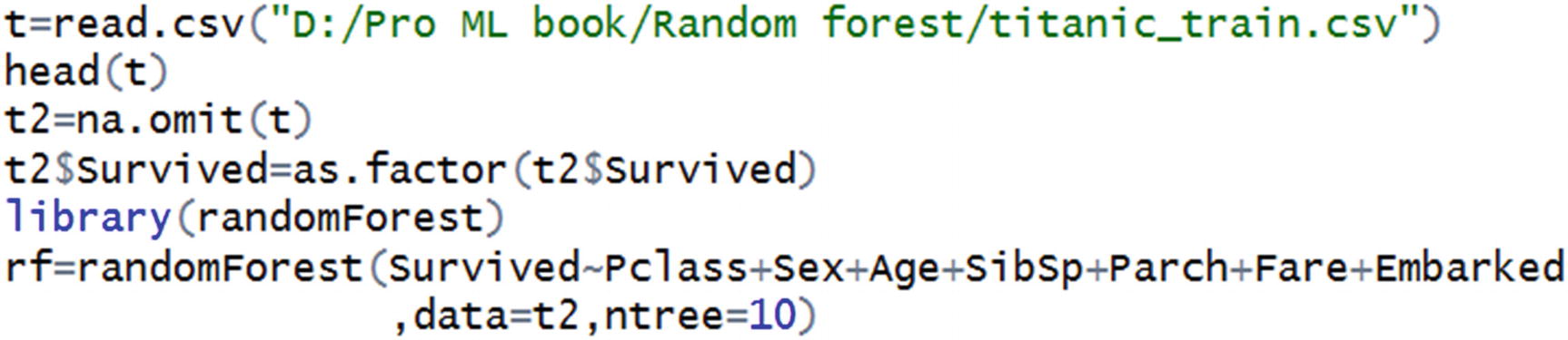
Now we can expect the random forest predictions to be made.
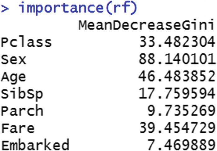
If we contrast the output with decision tree, one of the major drawbacks is that the decision tree output can be visualized as a tree, but random forest output cannot be visualized as a tree, because it is a combination of multiple decision trees. One way to understand the variable importance is by looking at how much of the decrease in overall impurity is because of splitting by the different variables.
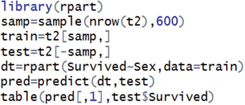
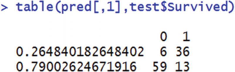
In the preceding code snippet, a sample of the original dataset is selected. That sample is considered as a training dataset, and the rest are considered as a test dataset.
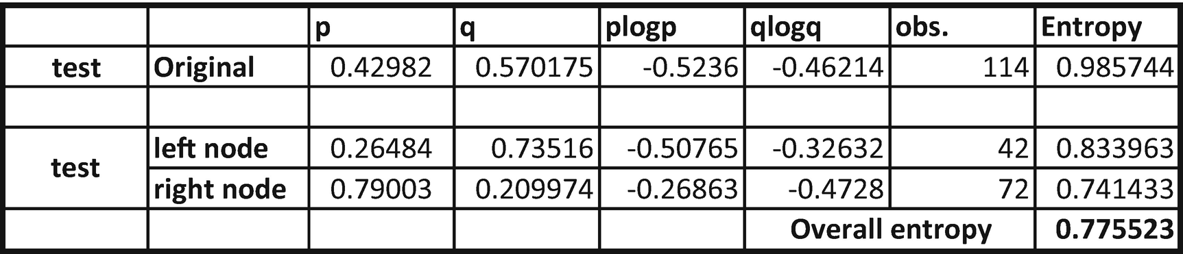
From the table, we can see that overall entropy reduces from 0.9857 to 0.7755.
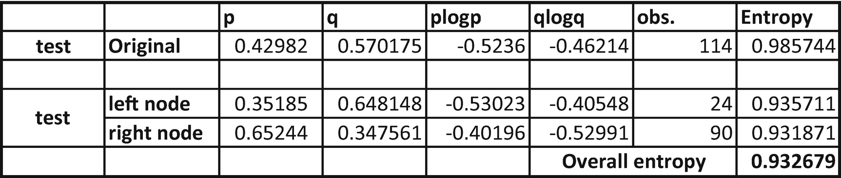
From the preceding table, we see that entropy reduced from 0.9857 to only 0.9326. So, there was a much lower reduction in entropy when compared to the variable Sex. That means Sex as a variable is more important than Embarked.
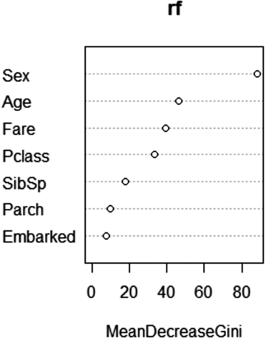
Variable importance plot
Parameters to Tune in a Random Forest
In the scenario just discussed, we noticed that random forest is based on decision tree, but on multiple trees running to produce an average prediction. Hence, the parameters that we tune in random forest would be very much the same as the parameters that are used to tune a decision tree.
Number of trees
Depth of tree
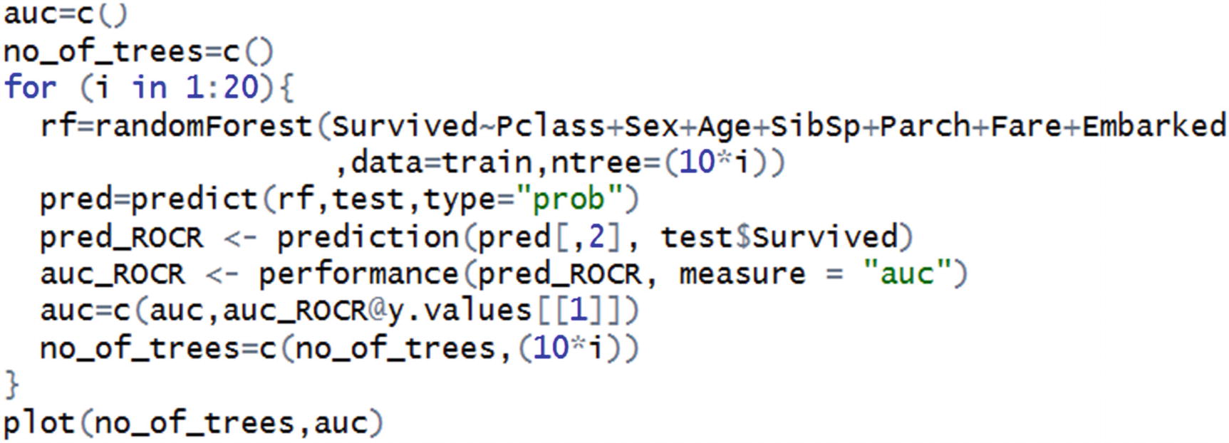
In the first two lines, we have initialized empty vectors that we will keep populating over the for loop of different numbers of trees. After initialization, we are running a loop where the number of trees is incremented by 10 in each step. After running the random forest, we are calculating the AUC value of the predictions on the test dataset and keep appending the values of AUC.
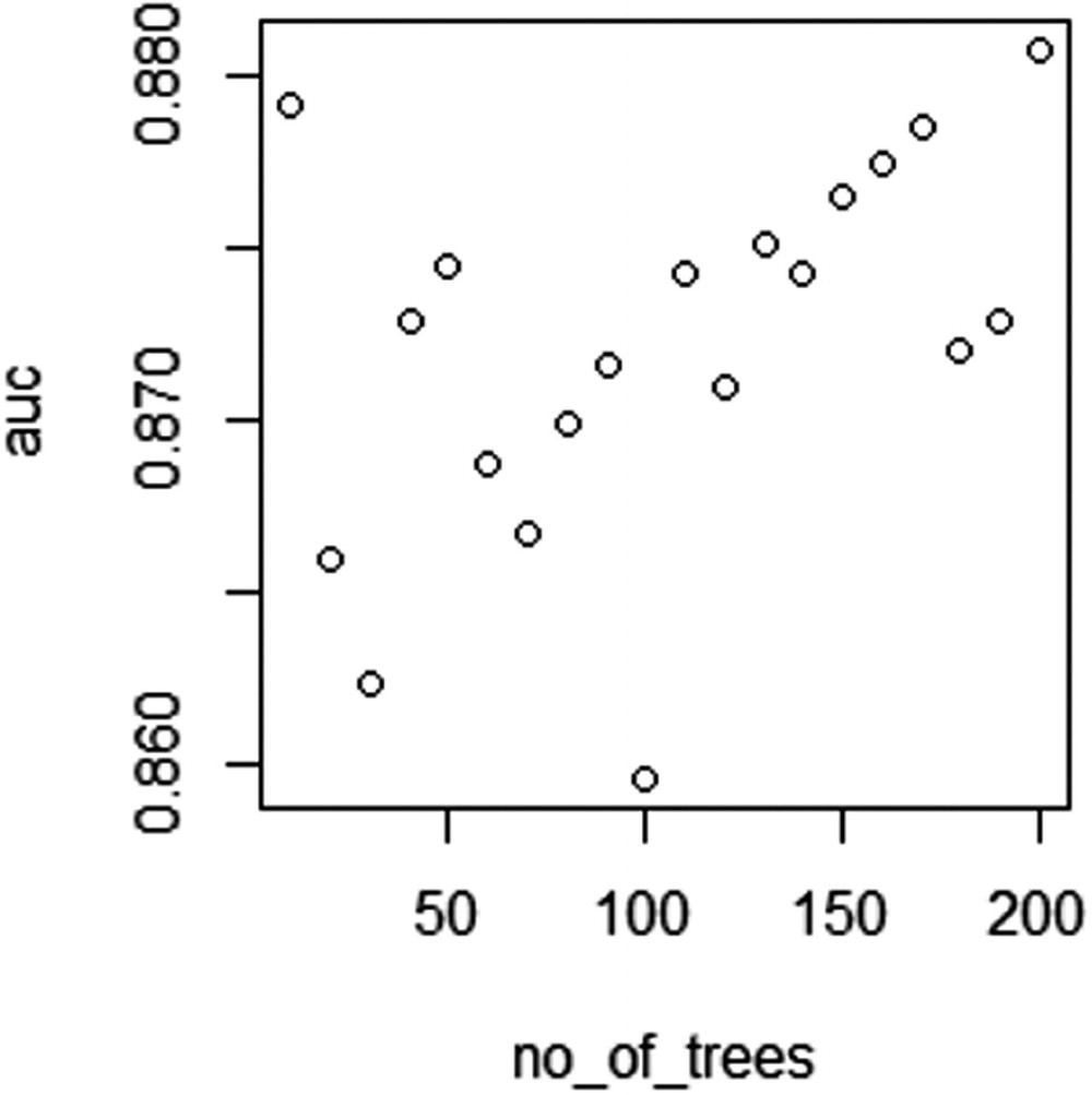
AUC over different number of trees
From Figure 5-2, we can see that as the number of trees increases, the AUC value of test dataset increases in general. But after a few more iterations, the AUC might not increase further.
Variation of AUC by Depth of Tree
In the previous section, we noted that the maximum value of AUC occurs when the number of trees is close to 200.
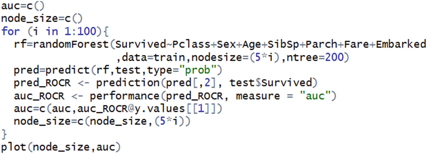
Note that the preceding code is very similar to the code we wrote for the variation in number of trees. The only addition is the parameter nodesize.
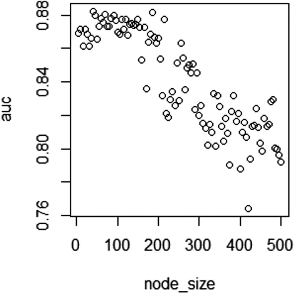
AUC over different node sizes
In Figure 5-3, note that as node size increases a lot, AUC of test dataset decreases.
Implementing a Random Forest in Python
Summary
In this chapter, we saw how random forest improves upon decision tree by taking an average prediction approach. We also saw the major parameters that need to be tuned within a random forest: depth of tree and the number of trees. Essentially, random forest is a bagging (bootstrap aggregating) algorithm—it combines the output of multiple decision trees to give the prediction.