
In the previous chapters, we’ve considered regression-based algorithms that optimize for a certain metric by varying coefficients or weights. A decision tree forms the basis of tree-based algorithms that help identify the rules to classify or forecast an event or variable we are interested in. Moreover, unlike linear or logistic regression, which are optimized for either regression or classification, decision trees are able to perform both.
The primary advantage of decision trees comes from the fact that they are business user friendly—that is, the output of a decision tree is intuitive and easily explainable to the business user.
How a decision tree works in classification and regression exercise
How a decision tree works when the independent variable is continuous or discrete
Various techniques involved in coming up with an optimal decision tree
Impact of various hyper-parameters on a decision tree
How to implement a decision tree in Excel, Python, and R
An example decision tree
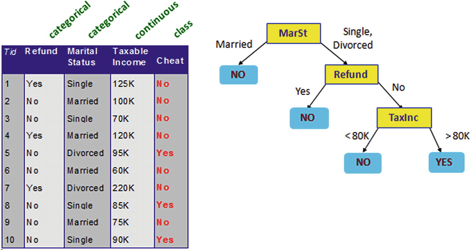
In Figure 4-1, we can see that a dataset (the table on the left) uses both a continuous variable (Taxable Income) and categorical variables (Refund, Marital Status) as independent variables to classify whether someone was cheating on their taxes or not (categorical dependent variable).
The tree on the right has a few components: root node, decision nodes, and leaf node (I talk more about these in next section) to classify whether someone would cheat (Yes/No).
- 1.
Someone with Marital Status of Yes is generally not a cheater.
- 2.
Someone who is divorced but also got a refund earlier also does not cheat.
- 3.
Someone who is divorced, did not get a refund, but has a taxable income of less than 80K is also not a cheater.
- 4.
Those who do not belong to any of the preceding categories are cheaters in this particular dataset.
Similar to regression, where we derived an equation (for example, to predict credit default based on customer characteristics) a decision tree also works to predict or forecast an event based on customer characteristics (for example, marital status, refund, and taxable income in the previous example).
When a new customer applies for a credit card, the rules engine (a decision tree running on the back end) would check whether the customer would fall in the risky bucket or the non-risky bucket after passing through all the rules of the decision tree. After passing through the rules, the system would approve or deny the credit card based on the bucket a user falls into.
Obvious advantages of decision trees are the intuitive output and visualization that help a business user make a decision. Decision trees are also less sensitive to outliers in cases of classification than a typical regression technique. Moreover, a decision tree is one of the simpler algorithms in terms of building a model, interpreting a model, or even implementing a model.
Components of a Decision Tree
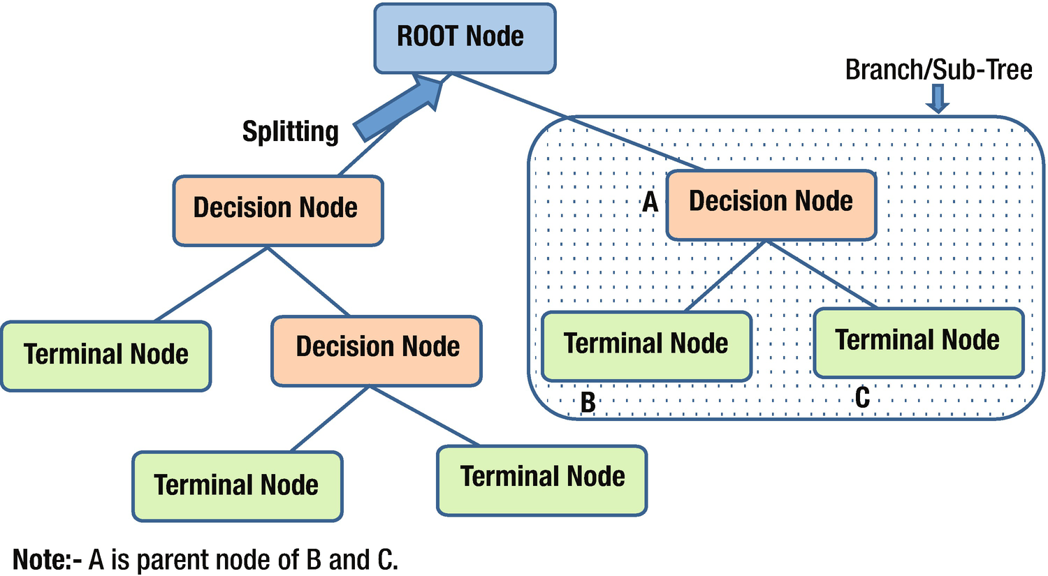
Components of a decision tree
Root node : This node represents an entire population or sample and gets divided into two or more homogeneous sets.
Splitting: A process of dividing a node into two or more sub-nodes based on a certain rule.
Decision node : When a sub-node splits into further sub-nodes, it is called a decision node.
Leaf / Terminal node : The final node in a decision tree.
Pruning: The process of removing sub-nodes from a decision node—the opposite of splitting.
Branch/Sub-tree: A subsection of an entire tree is called a branch or sub-tree.
Parent and child node: A node that is divided into sub-nodes is called the parent node of those sub-nodes, and the sub-nodes are the children of the parent node.
Classification Decision Tree When There Are Multiple Discrete Independent Variables
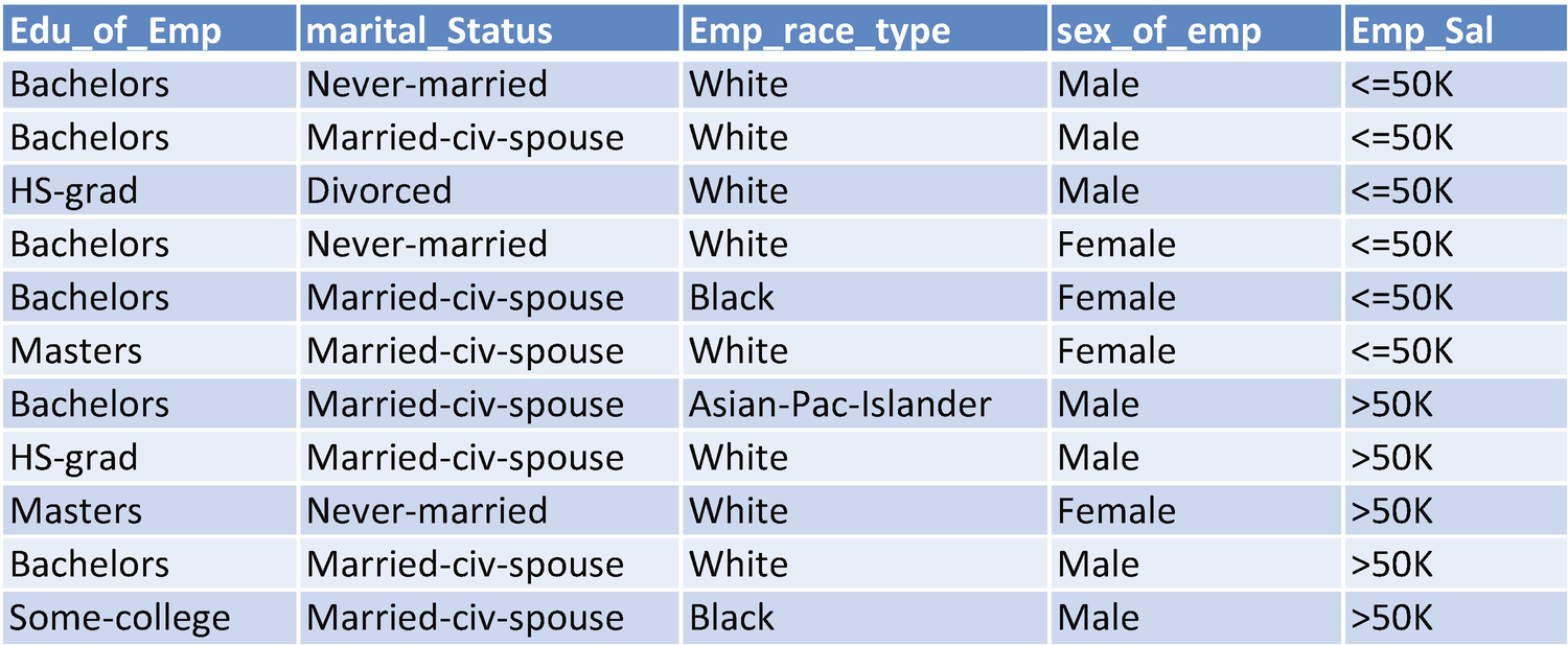
The criterion for splitting at a root node varies by the type of variable we are predicting, depending on whether the dependent variable is continuous or categorical. In this section, we’ll look at how splitting happens from the root node to decision nodes by way of an example. In the example, we are trying to predict employee salary (emp_sal) based on a few independent variables (education, marital status, race, and sex).
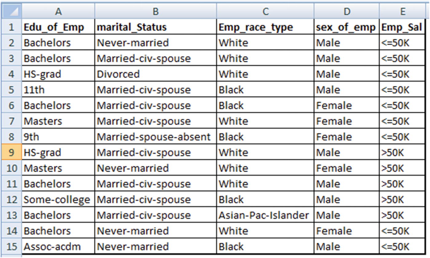
Here, Emp_sal is the dependent variable, and the rest of the variables are independent variables.
When splitting the root node (the original dataset), you first need to determine the variable based on which the first split has to be made—for example, whether you will split based on education, marital status, race, or sex. To come up with a way of shortlisting one independent variable over the rest, we use the information gain criterion.
Information Gain
Information gain is best understood by relating it to uncertainty. Let’s assume that there are two parties contesting in elections being conducted in two different states. In one state the chance of a win is 50:50 for each party, whereas in another state the chance of a win for party A is 90% and for party B it’s 10%.
If we were to predict the outcome of elections, the latter state is much easier to predict than the former because uncertainty is the least (the probability of a win for party A is 90%) in that state. Thus, information gain is a measure of uncertainty after splitting a node.
Calculating Uncertainty: Entropy

where p is the probability of event 1 happening, and q is the probability of event 2 happening.
Scenario | Party A uncertainty | Party B uncertainty | Overall uncertainty |
|---|---|---|---|
Equal chances of win | −0.5log2(0.5) = 0.5 | −0.5log2(0.5) = 0.5 | 0.5 + 0.5 =1 |
90% chances of win for party A | −0.9log2(0.9) = 0.1368 | −0.1log2(0.1) = 0.3321 | 0.1368 + 0.3321 = 0.47 |
We see that based on the previous equation, the second scenario has less overall uncertainty than the first, because the second scenario has a 90% chance of party A’s win.
Calculating Information Gain
We can visualize the root node as the place where maximum uncertainty exists. As we intelligently split further, the uncertainty decreases. Thus, the choice of split (the variable the split should be based on) depends on which variables decrease uncertainty the most.
To see how the calculation happens, let’s build a decision tree based on our dataset.
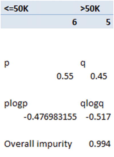
Uncertainty in the Original Dataset
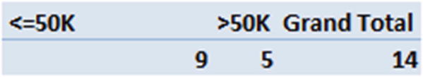
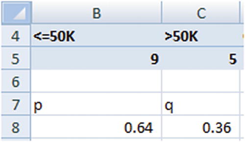
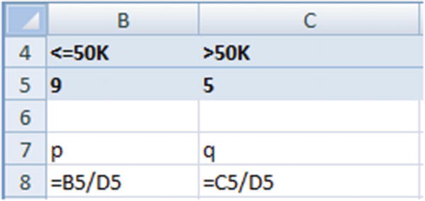
Uncertainty in <=50K | Uncertainty in >50K | Overall uncertainty |
–0.64 × log2(0.64) = 0.41 | −0.36 × log2(0.36) = 0.53 | 0.41 + 0.53 = 0.94 |
The overall uncertainty in the root node is 0.94.
To see the process of shortlisting variables in order to complete the first step, we’ll figure out the amount by which overall uncertainty decreases if we consider all four independent variables for the first split. We’ll consider education for the first split (we’ll figure out the improvement in uncertainty), next we’ll consider marital status the same way, then race, and finally the sex of the employee. The variable that reduces uncertainty the most will be the variable we should use for the first split.
Measuring the Improvement in Uncertainty
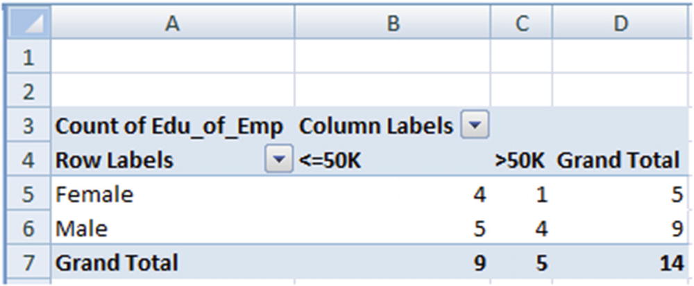
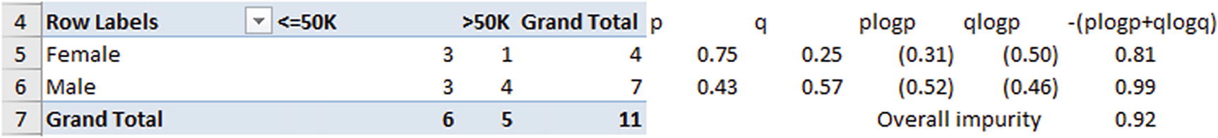
Sex | P | Q | –(plog2p) | –(qlog2q) | –(plog2p+qlog2q) | Weighted uncertainty |
|---|---|---|---|---|---|---|
Female | 4/5 | 1/5 | 0.257 | 0.46 | 0.72 | 0.72 × 5/14 = 0.257 |
Male | 5/9 | 4/9 | 0.471 | 0.52 | 0.99 | 0.99 × 9/14 = 0.637 |
Overall | 0.894 |
A similar calculation to measure the overall uncertainty of all the variables would be done. The information gain if we split the root node by the variable Sex is as follows:
(Original entropy – Entropy if we split by the variable Sex) = 0.94 – 0.894 = 0.046
Based on the overall uncertainty, the variable that maximizes the information gain (the reduction in uncertainty) would be chosen for splitting the tree.
Variable | Overall uncertainty | Reduction in uncertainty from root node |
|---|---|---|
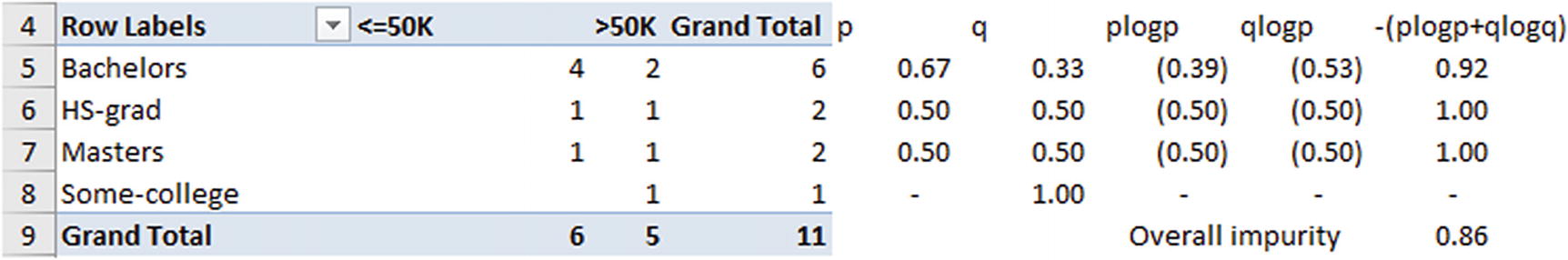
Education | 0.679 | 0.94 – 0.679 = 0.261 |
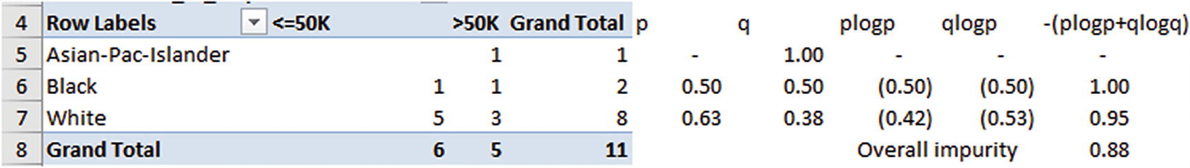
Marital status | 0.803 | 0.94 – 0.803 = 0.137 |
Race | 0.803 | 0.94 – 0.803 = 0.137 |
Sex | 0.894 | 0.94 – 0.894 = 0.046 |
From that we can observe that the splitting decision should be based on Education and not any other variable, because it is the variable that reduces the overall uncertainty by the most (from 0.94 to 0.679).
Once a decision about the split has been made, the next step (in the case of variables that have more than two distinct values—education in our example) would be to determine which unique value should go to the right decision node and which unique value should go to the left decision node after the root node.
Distinct value | % of obs. <=50K |
|---|---|
11th | 100% |
9th | 100% |
Assoc-acdm | 100% |
Bachelors | 67% |
HS-grad | 50% |
Masters | 50% |
Some-college | 0% |
Overall | 64% |
Which Distinct Values Go to the Left and Right Nodes
In the preceding section, we concluded that education is the variable on which the first split in the tree would be made. The next decision to be made is which distinct values of education go to the left node and which distinct values go to the right node.
The Gini impurity metric comes in handy in such scenario.
Gini Impurity
Gini impurity refers to the extent of inequality within a node. If a node has all values that belong to one class over the other, it is the purest possible node. If a node has 50% observations of one class and the rest of another class, it is the most impure form of a node.
Gini impurity is defined as  where p and q are the probabilities associated with each class.
P | Q | Gini index value |
|---|---|---|
0 | 1 | 1 – 02 – 12 = 0 |
1 | 0 | 1 – 12 – 02 =0 |
0.5 | 0.5 | 1 – 0.52 – 0.52 = 0.5 |
Let’s use Gini impurity for the employee salary prediction problem: From the information gain calculation in the previous section, we observed that Education is the variable used as the first split.
# of observations | Left node | Right node | Impurity | # of obs | ||||||||
|---|---|---|---|---|---|---|---|---|---|---|---|---|
<=50K | >50K | Grand Total | p | q | p | q | Left node | Right node | Left node | Right node | Weighted impurity | |
11th | 1 | 1 | 100% | 0% | 62% | 38% | - | 0.47 | 1 | 13 | 0.44 | |
9th | 1 | 1 | 100% | 0% | 58% | 42% | - | 0.49 | 2 | 12 | 0.42 | |
Assoc-acdm | 1 | 1 | 100% | 0% | 55% | 45% | - | 0.50 | 3 | 11 | 0.39 | |
Bachelors | 4 | 2 | 6 | 78% | 22% | 40% | 60% | 0.35 | 0.48 | 9 | 5 | 0.39 |
HS-grad | 1 | 1 | 2 | 73% | 27% | 33% | 67% | 0.40 | 0.44 | 11 | 3 | 0.41 |
Masters | 1 | 1 | 2 | 69% | 31% | 0% | 100% | 0.43 | - | 13 | 1 | 0.40 |
Some-college | 1 | 1 | ||||||||||
- 1.
Rank order the distinct values by the percentage of observations that belong to a certain class.
This would result in the distinct values being reordered as follows:Distinct value
% of obs <= 50K
11th
100%
9th
100%
Assoc-acdm
100%
Bachelors
67%
HS-grad
50%
Masters
50%
Some-college
0%
- 2.
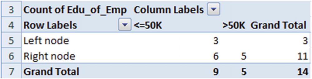
In the first step, let’s assume that only the distinct values that correspond to 11th go to the left node, and the rest of the distinct observations correspond to the right node.
Impurity in the left node is 0 because it has only one observation, and there will be some impurity in the right node because eight observations belong to one class and five belong to another class.
- 3.
Overall impurity is calculated as follows:
((Impurity in left node × # of obs. in left node) + (Impurity in right node × # of obs. in right node)) / (total no. of obs.)
- 4.
We repeat steps 2 and 3 but this time we include both 11th and 9th in the left node and the rest of the distinct values in the right node.
- 5.
The process is repeated until all the distinct values are considered in the left node.
- 6.
The combination that has the least overall weighted impurity is the combination that will be chosen in the left node and right node.
In our example, the combination of {11th,9th,Assoc-acdm} goes to the left node and the rest go to the right node as this combination has the least weighted impurity.
Splitting Sub-nodes Further
- 1.
Use the information gain metric to identify the variable that should be used to split the data.
- 2.
Use the Gini index to figure out the distinct values within that variable that should belong to the left node and the ones that should belong to the right node.
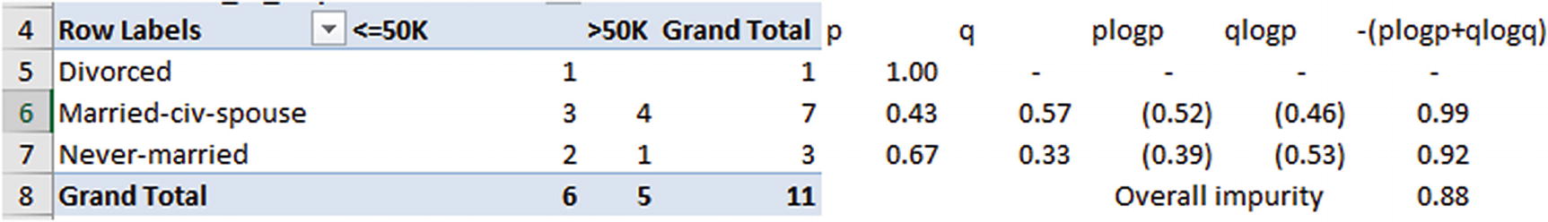
The overall impurity in the parent node for the preceding dataset is as follows: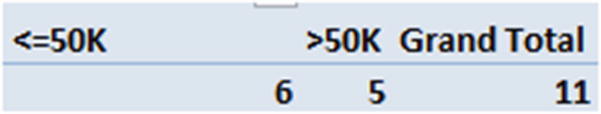
Now that the overall impurity is ~0.99, let’s look at the variable that reduces the overall impurity by the most. The steps we would go through would be the same as in the previous iteration on the overall dataset. Note that the only difference between the current version and the previous one is that in the root node the total dataset is considered, whereas in the sub-node only a subset of the data is considered.
From the above, we notice that employee education as a variable is the one that reduces impurity the most from the parent node—that is, the highest information gain is obtained from the employee education variable.
Notice that, coincidentally, the same variable happened to split the dataset twice, both in the parent node and in the sub-node. This pattern might not be repeated on a different dataset.
When Does the Splitting Process Stop?
Theoretically, the process of splitting can happen until all the terminal (leaf/last) nodes of a decision tree are pure (they all belong to one class or the other).
However, the disadvantage of such process is that it overfits the data and hence might not be generalizable. Thus, a decision tree is a trade-off between the complexity of the tree (the number of terminal nodes in a tree) and its accuracy. With a lot of terminal nodes, the accuracy might be high on training data, but the accuracy on validation data might not be high.
This brings us to the concept of the complexity parameter of a tree and out-of-bag validation. As the complexity of a tree increases—that is, the tree’s depth gets higher—the accuracy on the training dataset would keep increasing, but the accuracy on the test dataset might start getting lower beyond certain depth of the tree.
The splitting process should stop at the point where the validation dataset accuracy does not improve any further.
Classification Decision Tree for Continuous Independent Variables
So far, we have considered that both the independent and dependent variables are categorical. But in practice we might be working on continuous variables too, as independent variables. This section talks about how to build a decision tree for a continuous variable.
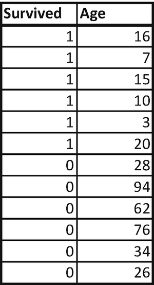
In this dataset, we’ll try to predict whether someone would survive or not based on the Age variable.
- 1.Sort the dataset by increasing independent variable. The dataset thus transforms into the following:
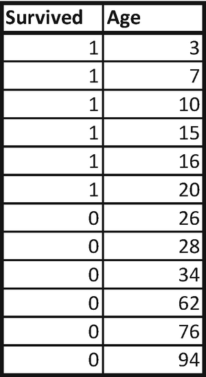
- 2.
Test out multiple rules. For example, we can test the impurity in both left and right nodes when Age is less than 7, less than 10 and so on until Age less than 94.
- 3.Calculate Gini impurity:
# of obs
Left node
Right node
Overall impurtiy
Survived
Count of Survived2
Left node
Right node
p
q
Impurity
p
q
Impurity
3
1
1
11
7
1
1
2
10
100%
0%
-
40%
60%
0.48
0.44
10
1
1
3
9
100%
0%
-
33%
67%
0.44
0.36
15
1
1
4
8
100%
0%
-
25%
75%
0.38
0.27
16
1
1
5
7
100%
0%
-
14%
86%
0.24
0.16
20
1
1
6
6
100%
0%
-
0%
100%
-
-
26
0
1
7
5
86%
14%
0.24
0%
100%
-
0.13
28
0
1
8
4
75%
25%
0.38
0%
100%
-
0.24
34
0
1
9
3
67%
33%
0.44
0%
100%
-
0.32
62
0
1
10
2
60%
40%
0.48
0%
100%
-
0.39
76
0
1
11
1
55%
45%
0.50
0%
100%
-
0.45
94
0
1
12
From the preceding table, we should notice that Gini impurity is the least when the independent variable value is less than 26.
Thus we will choose Age less than 26 as the rule that splits the original dataset.
Note that both Age > 20 as well as Age < 26 split the dataset to the same extent of error rate. In such a scenario, we need to come up with a way to choose the one rule between the two rules. We’ll take the average of both rules, so Age <= 23 would be the rule that is midway between the two rules and hence a better rule than either of the two.
Classification Decision Tree When There Are Multiple Independent Variables
Survived | Age | Unknown |
|---|---|---|
1 | 30 | 79 |
1 | 7 | 67 |
1 | 100 | 53 |
1 | 15 | 33 |
1 | 16 | 32 |
1 | 20 | 5 |
0 | 26 | 14 |
0 | 28 | 16 |
0 | 34 | 70 |
0 | 62 | 35 |
0 | 76 | 66 |
0 | 94 | 22 |
- 1.
Identify the variable that should be used for the split first by using information gain.
- 2.
Once a variable is identified, in the case of discrete variables, identify the unique values that should belong to the left node and the right node.
- 3.
In the case of continuous variables, test out all the rules and shortlist the rule that results in minimal overall impurity.
In this case, we’ll reverse the scenario—that is, we’ll first find out the rule of splitting to the left node and right node, if we were to split on any of the variables. Once the left and right nodes are figured, we’ll calculate the information gain obtained by the split and thus shortlist the variable that should be slitting the overall dataset.
Age | Survived |
|---|---|
7 | 1 |
15 | 1 |
16 | 1 |
20 | 1 |
26 | 0 |
28 | 0 |
30 | 1 |
34 | 0 |
62 | 0 |
76 | 0 |
94 | 0 |
100 | 1 |
# of obs | Left node | Right node | |||||||||
|---|---|---|---|---|---|---|---|---|---|---|---|
Age | Survived | Count of Survived2 | Left node | Right node | p | q | Impurity | p | q | Impurity | Overall impurtiy |
7 | 1 | 1 | 11 | ||||||||
15 | 1 | 1 | 2 | 10 | 100% | 0% | - | 40% | 60% | 0.48 | 0.40 |
16 | 1 | 1 | 3 | 9 | 100% | 0% | - | 33% | 67% | 0.44 | 0.33 |
20 | 1 | 1 | 4 | 8 | 100% | 0% | - | 25% | 75% | 0.38 | 0.25 |
26 | 0 | 1 | 5 | 7 | 80% | 20% | 0.32 | 29% | 71% | 0.41 | 0.37 |
28 | 0 | 1 | 6 | 6 | 67% | 33% | 0.44 | 33% | 67% | 0.44 | 0.44 |
30 | 1 | 1 | 7 | 5 | 71% | 29% | 0.41 | 20% | 80% | 0.32 | 0.37 |
34 | 0 | 1 | 8 | 4 | 63% | 38% | 0.47 | 25% | 75% | 0.38 | 0.44 |
62 | 0 | 1 | 9 | 3 | 56% | 44% | 0.49 | 33% | 67% | 0.44 | 0.48 |
76 | 0 | 1 | 10 | 2 | 50% | 50% | 0.50 | 50% | 50% | 0.50 | 0.50 |
94 | 0 | 1 | 11 | 1 | 45% | 55% | 0.50 | 100% | 0% | - | 0.45 |
100 | 1 | 1 | 12 | ||||||||
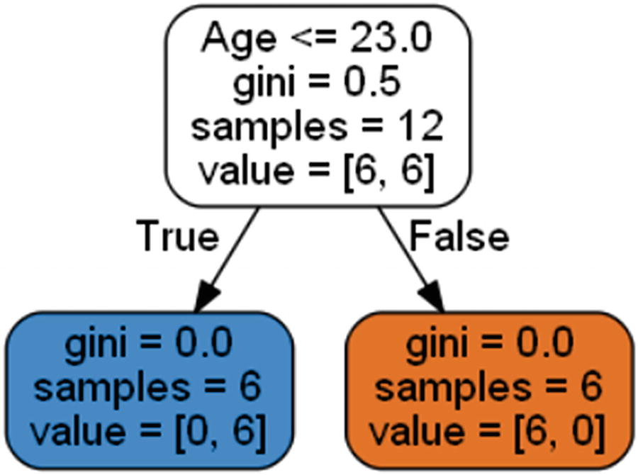
From the data, we can see that the rule derived should be Age <= 20 or Age >= 26. So again, we’ll go with the middle value: Age <= 23.
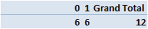
Given that both 0 and 1 are 6 in number (50% probability for each), the overall entropy comes out to be 1.
Survived | |||||||
|---|---|---|---|---|---|---|---|
0 | 1 | Grand Total | p | q | -(plogp+qlogq) | wegihted entropy | |
Age<=23 | 4 | 4 | 0 | 1 | 0 | 0 | |
Age>23 | 6 | 2 | 8 | 0.75 | 0.25 | 0.811278 | 0.540852 |
Grand Total | 6 | 6 | 12 | Overall entropy | 0.540852 | ||
# of obs | Left node | Right node | |||||||||
|---|---|---|---|---|---|---|---|---|---|---|---|
Unknwon | Survived | Count of Survived2 | Left node | Right node | p | q | Impurity | p | q | Impurity | Overall impurtiy |
5 | 1 | 1 | 11 | ||||||||
14 | 0 | 1 | 2 | 10 | 50% | 50% | 0.50 | 50% | 50% | 0.50 | 0.50 |
16 | 0 | 1 | 3 | 9 | 33% | 67% | 0.44 | 56% | 44% | 0.49 | 0.48 |
22 | 0 | 1 | 4 | 8 | 25% | 75% | 0.38 | 63% | 38% | 0.47 | 0.44 |
32 | 1 | 1 | 5 | 7 | 40% | 60% | 0.48 | 57% | 43% | 0.49 | 0.49 |
33 | 1 | 1 | 6 | 6 | 50% | 50% | 0.50 | 50% | 50% | 0.50 | 0.50 |
35 | 0 | 1 | 7 | 5 | 43% | 57% | 0.49 | 60% | 40% | 0.48 | 0.49 |
53 | 1 | 1 | 8 | 4 | 50% | 50% | 0.50 | 50% | 50% | 0.50 | 0.50 |
66 | 0 | 1 | 9 | 3 | 44% | 56% | 0.49 | 67% | 33% | 0.44 | 0.48 |
67 | 1 | 1 | 10 | 2 | 50% | 50% | 0.50 | 50% | 50% | 0.50 | 0.50 |
70 | 0 | 1 | 11 | 1 | 45% | 55% | 0.50 | 100% | 0% | - | 0.45 |
79 | 1 | 1 | 12 | ||||||||
Thus, all values less than or equal to 22 belong to one group (left node), and the rest belong to another group (right node). Note that, practically we would go with a mid value between 22 and 32.
Survived | |||||||
|---|---|---|---|---|---|---|---|
0 | 1 | Grand Total | p | q | -(plogp+qlogq) wegihted entropy | ||
Unknown<=22 | 3 | 1 | 4 | 0.75 | 0.25 | 0.81 | 0.27 |
Unknown>22 | 3 | 5 | 8 | 0.375 | 0.625 | 0.95 | 0.64 |
Grand Total | 6 | 6 | 12 | Overall entropy | 0.91 | ||
From the data, we see that information gain, due to splitting by the Unknown variable, is only 0.09. Hence, the split would be based on Age, not Unknown.
Classification Decision Tree When There Are Continuous and Discrete Independent Variables
We’ve seen ways of building classification decision tree when all independent variables are continuous and when all independent variables are discrete.
- 1.
For the continuous independent variables, we calculate the optimal splitting point.
- 2.
Once the optimal splitting point is calculated, we calculate the information gain associated with it.
- 3.
For the discrete variable, we calculate the Gini impurity to figure out the grouping of distinct values within the respective independent variable.
- 4.
Whichever is the variable that maximizes information gain is the variable that splits the decision tree first.
- 5.
We continue with the preceding steps in further building the sub-nodes of the tree.
What If the Response Variable Is Continuous?
If the response variable is continuous , the steps we went through in building a decision tree in the previous section remain the same, except that instead of calculating Gini impurity or information gain, we calculate the squared error (similar to the way we minimized sum of squared error in regression techniques). The variable that reduces the overall mean squared error of the dataset will be the variable that splits the dataset.
variable | response |
|---|---|
-0.37535 | 1590 |
-0.37407 | 2309 |
-0.37341 | 815 |
-0.37316 | 2229 |
-0.37263 | 839 |
-0.37249 | 2295 |
-0.37248 | 1996 |
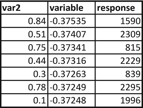
Here, the independent variable is named variable, and the dependent variable is named response. The first step would be to sort the dataset by the independent variable, as we did in the classification decision tree example.
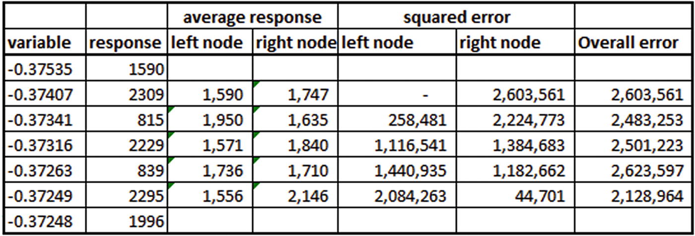
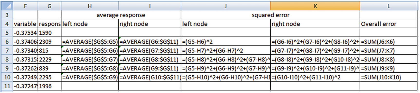
From the preceding, we see that the minimal overall error occurs when variable < -0.37249. So, the points that belong to the left node will have an average response of 1,556, and the points that belong to the right node will have an average response of 2,146. Note that 1,556 is the average response of all the variable values that are less than the threshold that we derived earlier. Similarly, 2,146 is the average response of all the variable values that are greater than or equal to the threshold that we derived (0.37249).
Continuous Dependent Variable and Multiple Continuous Independent Variables
In classification, we considered information gain as a metric to decide the variable that should first split the original dataset. Similarly, in the case of multiple competing independent variables for a continuous variable prediction, we’ll shortlist the variable that results in least overall error.
We already calculated the overall error for various possible rules of variable in the previous section. Let’s calculate the overall error for the various possible rules of var2.
var2 | response |
|---|---|
0.1 | 1996 |
0.3 | 839 |
0.44 | 2229 |
0.51 | 2309 |
0.75 | 815 |
0.78 | 2295 |
0.84 | 1590 |
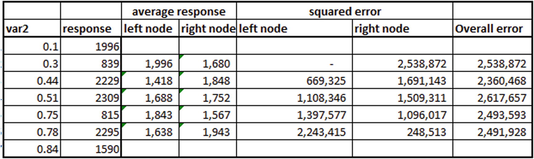
Note that overall error is the least when var2 < 0.44. However, when we compare the least overall error produced by variable and the least overall error produced by var2, variable produces the least overall error and so should be the variable that splits the dataset.
Continuous Dependent Variable and Discrete Independent Variable
var | response |
|---|---|
a | 1590 |
b | 2309 |
c | 815 |
a | 2229 |
b | 839 |
c | 2295 |
a | 1996 |
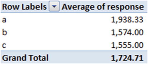
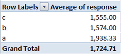
Now we’ll calculate the optimal left node and right node combination. In the first scenario, only c would be in the left node and a,b will be in the right node. The average response in left node will be 1555, and the average response in right node will be the average of {1574,1938} = {1756}.
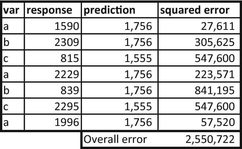
In the second scenario, we’ll consider both {c,b} to belong to the left node and {a} to belong to the right node. In this case, the average response in left node will be the average of {1555,1574} = {1564.5}
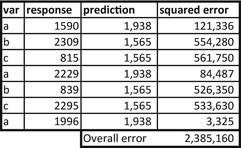
We can see that the latter combination of left and right nodes yields the lesser overall error when compared to the previous combination. So, the ideal split in this case would be {b,c} belonging to one node and {a} belonging to another node.
Continuous Dependent Variable and Discrete, Continuous Independent Variables
- 1.
Identify the optimal cut-off points for each variable individually.
- 2.
Understand the variable that reduces uncertainty the most.
The steps to be followed remain the same as in the previous sections.
Implementing a Decision Tree in R
The implementation of classification is different from the implementation of regression (continuous variable prediction). Thus, a specification of the type of model is required as an input.
The decision tree is implemented using the functions available in a package named rpart. The function that helps in building a decision tree is also named rpart. Note that in rpart we specify the method parameter.
A method anova is used when the dependent variable is continuous, and a method class is used when the dependent variable is discrete.
You can also specify the additional parameters: minsplit, minbucket, and maxdepth (more on these in the next section).
Implementing a Decision Tree in Python
The Python implementation of a classification problem would make use of the DecisionTreeClassifier function in the sklearn package (The code is available as “Decision tree.ipynb” in github):
For a regression problem, the Python implementation would make use of the DecisionTreeRegressor function in the sklearn package:
Common Techniques in Tree Building
Restricting the number of observations in each terminal node to a minimum number (at least 20 observations in a node, for example)
Specifying the maximum depth of a tree manually
Specifying the minimum number of observations in a node for the algorithm to consider further splitting
- 1.
The tree has a total of 90 depth levels (maxdepth = 90). In this scenario, the tree that gets constructed would have so many branches that it overfits on the training dataset but does not necessarily generalize on the test dataset.
- 2.
Similar to the problem with maxdepth, minimum number of observations in a terminal node could also lead to overfitting. If we do not specify maxdepth and have a small number in the minimum number of observations in the terminal node parameter, the resulting tree again is likely to be huge, with multiple branches, and will again be likely to result in a overfitting to a training dataset and not generalizing for a test dataset.
- 3.
Minimum number of observations in a node to further split is a parameter that is very similar to minimum observations in a node, except that this parameter restricts the number of observations in the parent node rather than the child node.
Visualizing a Tree Build
In R, one can plot the tree structure using the plot function available in the rpart package. The plot function plots the skeleton of the tree, and the text function writes the rules that are derived at various parts of the tree. Here’s a sample implementation of visualizing a decision tree:
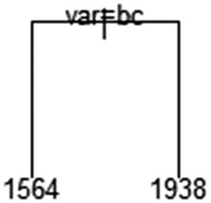
From this plot, we can deduce that when var is either of b or c, then the output is 1564. If not, the output is 1938.
In Python, one way to visualize a decision tree is by using a set of packages that have functions that help in display: Ipython.display, sklearn.externals.six, sklearn.tree, pydot, os.
In the preceding code, you would have to change the data frame name in place of (data.columns[1:]) that we used in the first code snippet. Essentially, we are providing the independent variable names as features.
In the second code snippet, you would have to specify the folder location at which graphviz was installed and change the decision tree name to the name that the user has given in the fourth line (replace dtree with the variable name that you have created for DecisionTreeRegressor or DecisionTreeClassifier).
The output of the code
Impact of Outliers on Decision Trees
In previous chapters, we’ve seen that outliers have a big impact in the case of linear regression. However, in a decision tree outliers have little impact for classification, because we look at the multiple possible rules and shortlist the one that maximizes the information gain after sorting the variable of interest. Given that we are sorting the dataset by independent variable, there is no impact of outliers in the independent variable.
However, an outlier in the dependent variable in the case of a continuous variable prediction would be challenging if there is an outlier in the dataset. That’s because we are using overall squared error as a metric to minimize. If the dependent variable contains an outlier, it causes similar issues like what we saw in linear regression.
Summary
Decision trees are simple to build and intuitive to understand. The prominent approaches used to build a decision tree are the combination of information gain and Gini impurity when the dependent variable is categorical and overall squared error when the dependent variable is continuous.