V Kishore AyyadevaraPro Machine Learning Algorithms https://doi.org/10.1007/978-1-4842-3564-5_10

10. Recurrent Neural Network

V Kishore Ayyadevara¹

(1)

Hyderabad, Andhra Pradesh, India

In Chapter 9, we looked at how convolutional neural networks (CNNs) improve upon the traditional neural network architecture for image classification. Although CNNs perform very well for image classification in which image translation and rotation are taken care of, they do not necessarily help in identifying temporal patterns. Essentially, one can think of CNNs as identifying static patterns.

Recurrent neural networks (RNNs) are designed to solve the problem of identifying temporal patterns.

In this chapter, you will learn the following:

Working details of RNN
Using embeddings in RNN
Generating text using RNN
Doing sentiment classification using RNN
Moving from RNN to LSTM

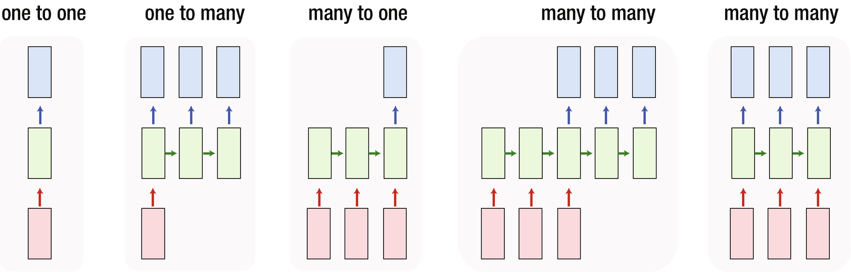
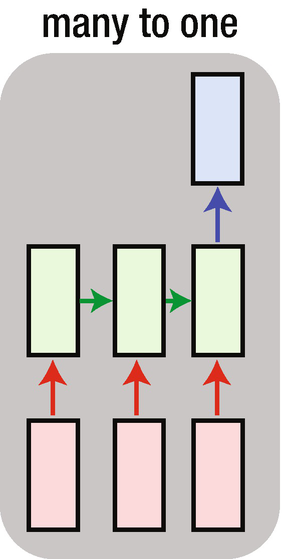
RNN can be architected in multiple ways. Some of the possible ways are shown in Figure 10-1.

../images/463052_1_En_10_Chapter/463052_1_En_10_Fig1_HTML.png — Figure 10-1
RNN examples

In Figure 10-1 note the following:

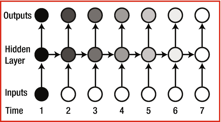
The boxes in the bottom are inputs
The boxes in the middle are hidden layers
The boxes at the top are outputs

An example of the one-to-one architecture shown is a typical neural network that we have looked at in chapter 7, with a hidden layer between the input and the output layer. An example of one-to-many RNN architecture would be to input an image and output the caption of the image. An example of many-to-one RNN architecture might be a movie review given as input and the movie sentiment (positive, negative or neutral review) as output. Finally, an example of many-to-many RNN architecture would be machine translation from one language to another language.

Understanding the Architecture

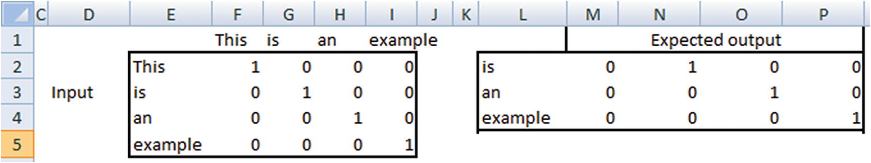
Let’s go through an example and look more closely at RNN architecture. Our task is as follows: “Given a string of words, predict the next word.” We’ll try to predict the word that comes after “This is an _____”. Let’s say the actual sentence is “This is an example.”

Traditional text mining techniques would solve the problem in the following way:

1.
Encode each word, leaving space for an extra word, if needed:

This: {1,0,0,0}
is: {0,1,0,0}
an: {0,0,1,0}
2.
Encode the sentence:

"This is an": {1,1,1,0}
3.
Create a training dataset:

Input --> {1,1,1,0}
Output --> {0,0,0,1}
4.
Build a model with input and output.

One of the major drawbacks here is that the input representation does not change if the input sentence is either “this is an” or “an is this” or “this an is”. We know that each of these is very different and cannot be represented by the same structure mathematically.

This realization calls for having a different architecture, one that looks more like Figure 10-2.

../images/463052_1_En_10_Chapter/463052_1_En_10_Fig2_HTML.png — Figure 10-2
A change in the architecture

In the architecture shown in Figure 10-2, each of the individual words in the sentence goes into a separate box among the three input boxes. Moreover, the structure of the sentence is preserved since “this” gets into the first box, “is” gets into the second box, and “an” gets into the third box.

The output “example” is expected in the output box at the top.

Interpreting an RNN

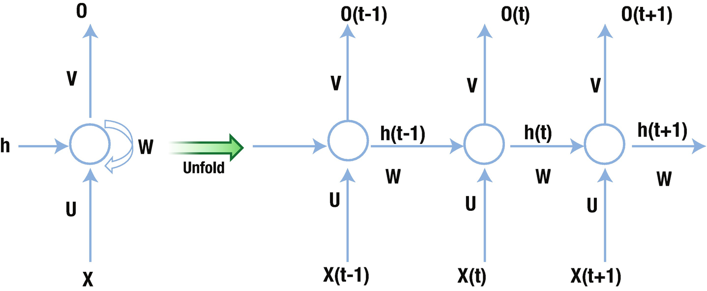
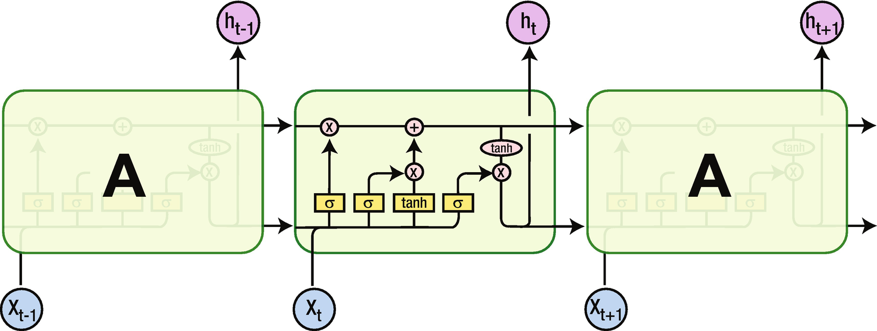
We can think of RNN as a mechanism to hold memory, where the memory is contained within the hidden layer. This is illustrated in Figure 10-3.

../images/463052_1_En_10_Chapter/463052_1_En_10_Fig3_HTML.png — Figure 10-3
Memory in the hidden layer

The network on the right in Figure 10-3 is an unrolled version of the network on the left. The network on the left is a traditional one, with one change: the hidden layer is connected to itself along with being connected to the input (the hidden layer is the circle in the figure).

Note that when a hidden layer is connected to itself along with input layer, it is connected to a “previous version” of the hidden layer and the current input layer. We can consider this phenomenon of the hidden layer being connect back to itself as the mechanism by which memory is created in RNN.

The weight U represents the weights that connect the input layer to the hidden layer, the weight W represents the hidden-layer-to-hidden-layer connection, and the weight V represents the hidden-layer-to-output-layer connection.

Why Store Memory?

There is a need to store memory because, in the preceding example and in text generation in general, the next word does not necessarily rely on the preceding word but the context of the few words preceding the word to predict.

Given that we are looking at the preceding words, there should be a way to keep them in memory so that we can predict the next word more accurately. Moreover, we should also have the memory in order—more often than not, more recent words are more useful in predicting the next word than the words that are far away from the word being predicted.

Working Details of RNN

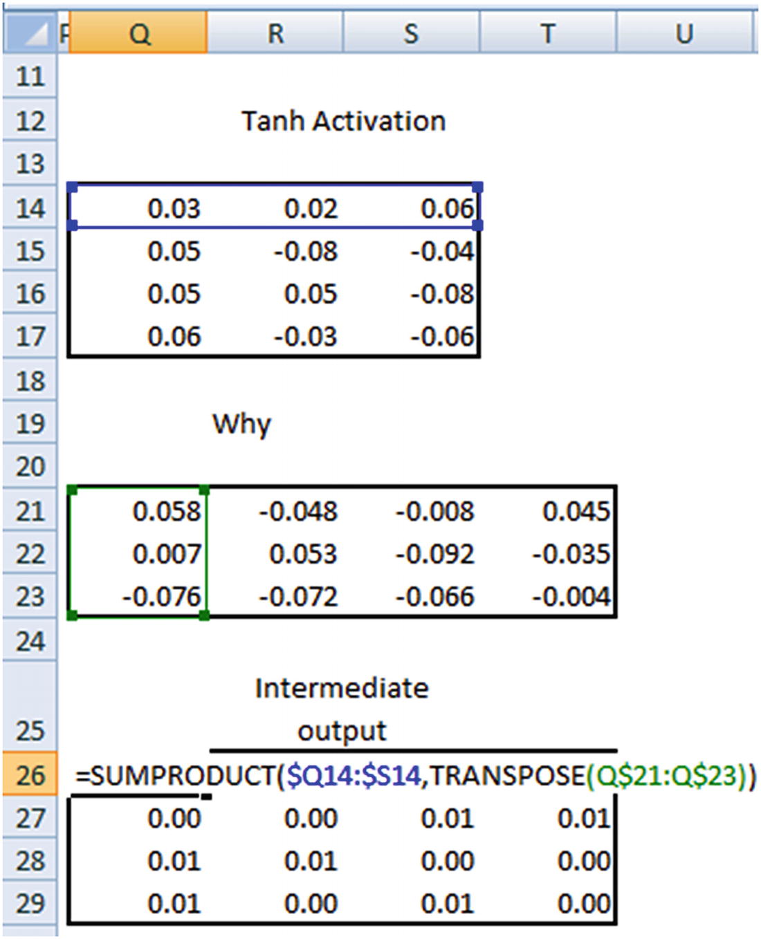
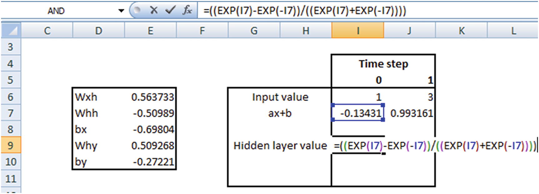
Note that a typical NN has an input layer followed by an activation in the hidden layer and then a softmax activation at the output layer. RNN is similar, but with memory. Let’s look at another example: “This is an example”. Given an input “This”, we are expected to predict “is” and similarly for an input “is”, we are expected to come up with a prediction of “an” and a prediction of “example” for “an” as input. The dataset is available as “RNN dimension intuition.xlsx” in github.

The encoded input and output words are as follows:

../images/463052_1_En_10_Chapter/463052_1_En_10_Figa_HTML.jpg

The RNN structure looks like Figure 10-4.

../images/463052_1_En_10_Chapter/463052_1_En_10_Fig4_HTML.png — Figure 10-4
The RNN structure

Let’s deconstruct the dimensions of each weight matrix associated:

../images/463052_1_En_10_Chapter/463052_1_En_10_Figb_HTML.jpg

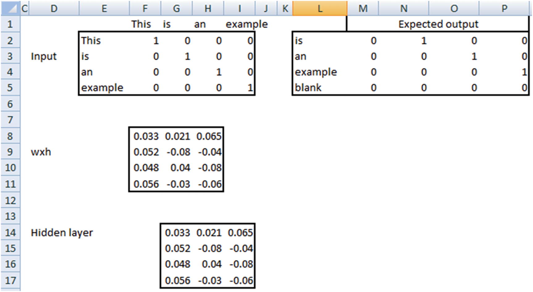
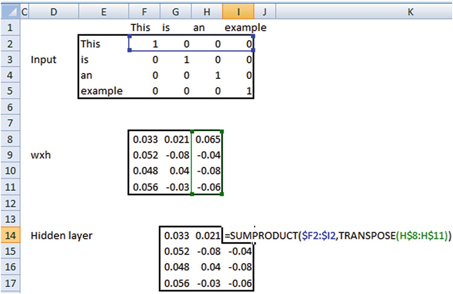
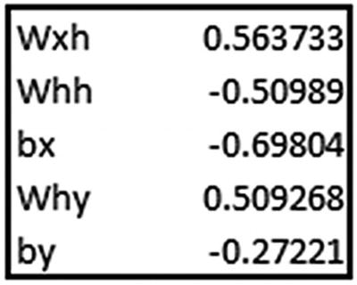
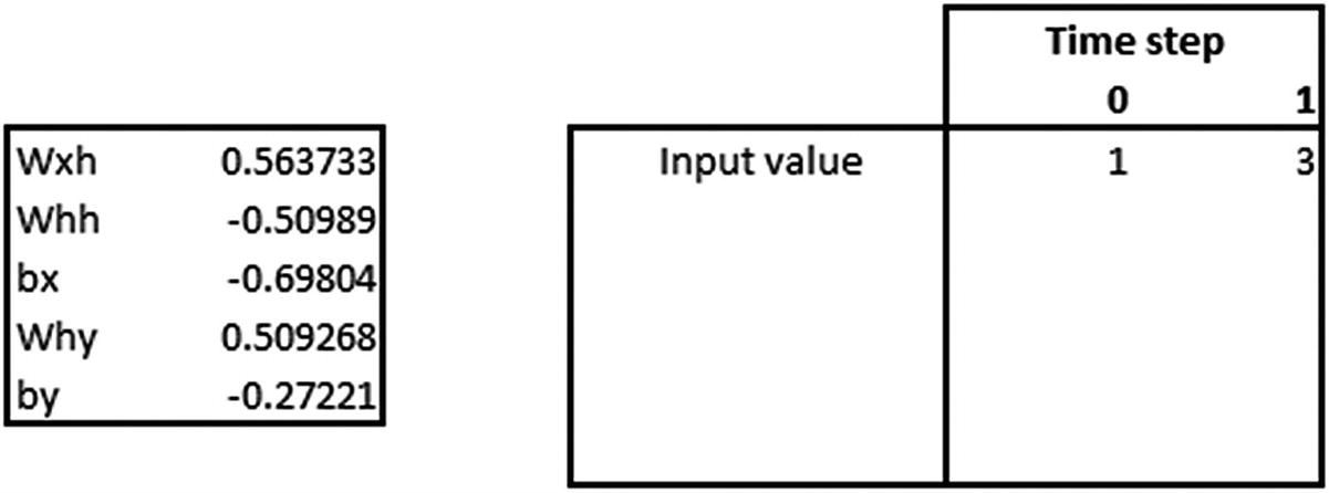
wxh is randomly initialized and 4 × 3 in dimension. Each input is 1 × 4 in dimension. Thus, the hidden layer, which is a matrix multiplication between the input and wxh, is 1 × 3 in dimension for each input row. The expected output is the one-hot encoded version of the word that comes next to the input word in our sentence. Note that, the last prediction “blank” is inaccurate because we have all 0s as expected output. Ideally, we would have a new column in the one-hot encoded version that takes care of all the unseen words. However, for the sake of understanding the working details of RNN we will keep it simple with 4 columns in expected output.

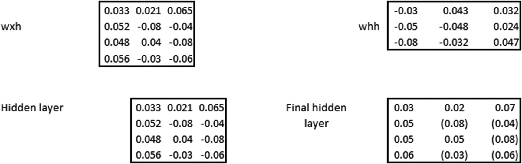
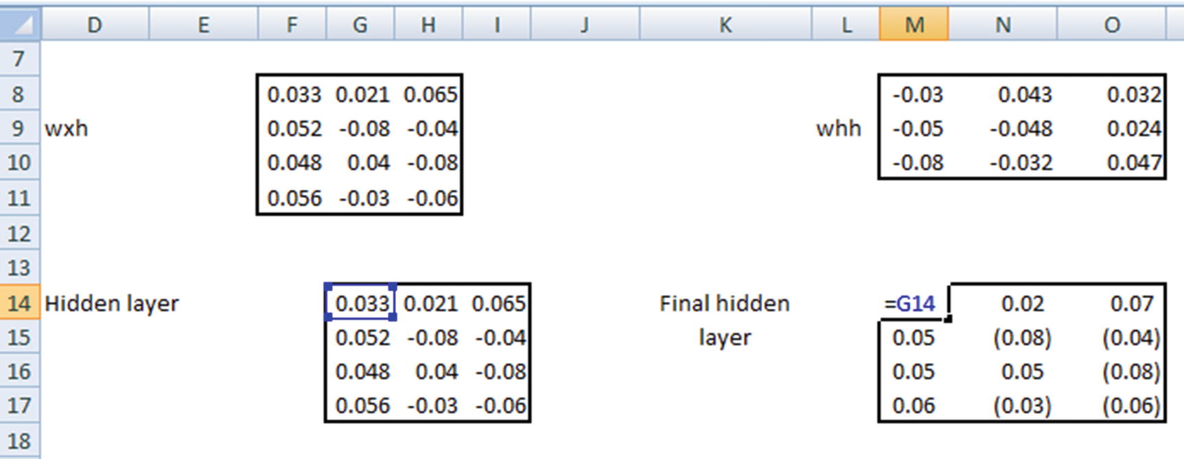
As we saw earlier, in RNN, a hidden layer is connected to another hidden layer when unrolled. Given that a hidden layer is connected to the next hidden layer, the weight (whh) associated with the connection between the previous hidden layer and the current hidden layer would be 3 × 3 in dimension, since a 1 × 3 matrix multiplied with 3 × 3 matrix would yield a 1 × 3 matrix. Final hidden layer calculations in the below picture are explained in subsequent pages.

../images/463052_1_En_10_Chapter/463052_1_En_10_Figc_HTML.jpg

Note that, wxh and whh are random initializations, whereas the hidden layer and the final hidden layer are calculated. We will look at how the calculations are done in the following pages.

The calculation for the hidden layer at various time steps is performed as follows:

${h}^{(t)}={\phi}_h\left({z}_h^{(t)}\right)={\phi}_h\left({W}_{xh}{x}^{(t)}+{W}_{hh}{h}^{\left(t-1\right)}\right)$

where ../images/463052_1_En_10_Chapter/463052_1_En_10_Figd_HTML.gif is an activation that is performed (tanh activation in general).

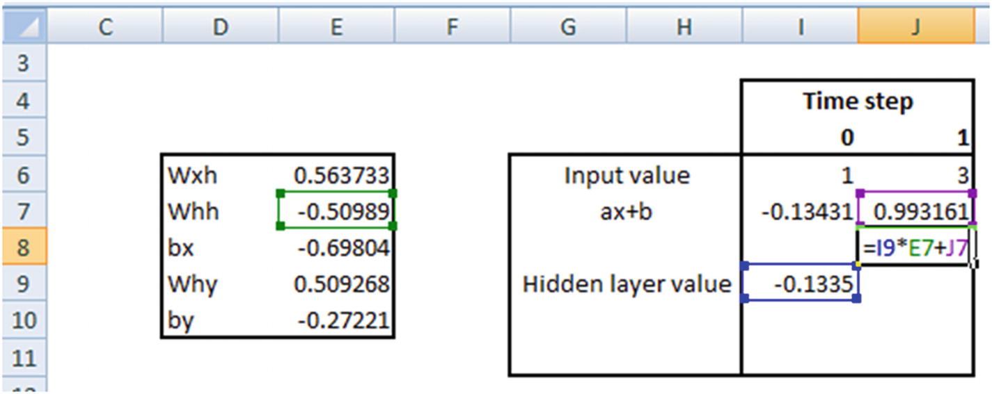
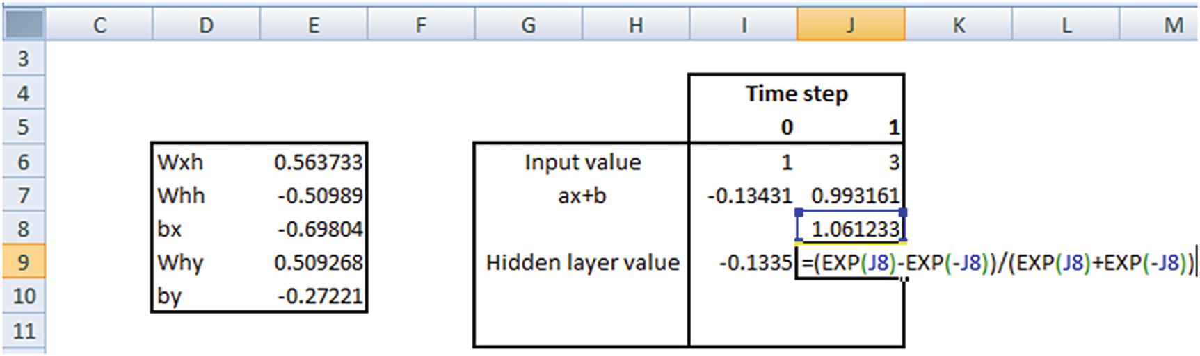
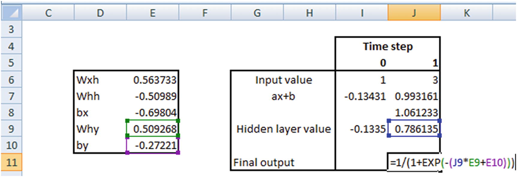
Calculation from the input layer to the hidden layer consists of two components:

Matrix multiplication of the input layer and wxh.
Matrix multiplication of hidden layer and whh.

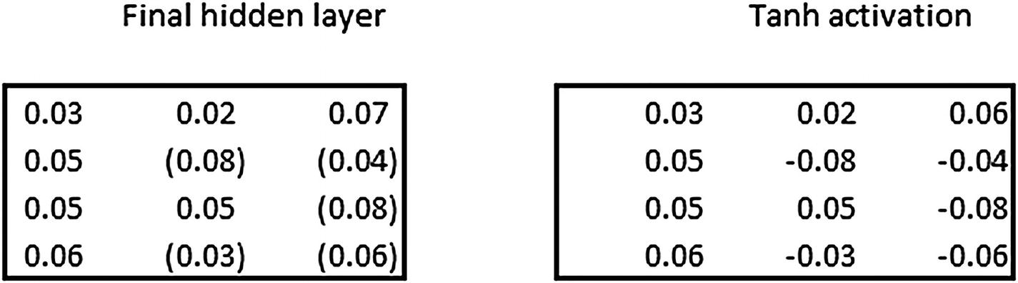
Final calculation of the hidden layer value at a given time step would be the summation of the preceding two matrix multiplications and passing the result through a tanh activation function.

Matrix multiplication of the input layer and wxh is shown here:

../images/463052_1_En_10_Chapter/463052_1_En_10_Fige_HTML.jpg

The following sections go through the calculation of the hidden layer value at different time steps.

Time Step 1

The hidden layer value at the first time step would be the value of matrix multiplication between the input layer and wxh (because there is no hidden layer value in the previous time step):

../images/463052_1_En_10_Chapter/463052_1_En_10_Figf_HTML.jpg

Time Step 2

Starting the second input, the hidden layer consists of the hidden layer component of the current time step and the hidden layer component coming from the previous time step:

../images/463052_1_En_10_Chapter/463052_1_En_10_Figg_HTML.jpg

../images/463052_1_En_10_Chapter/463052_1_En_10_Figh_HTML.jpg

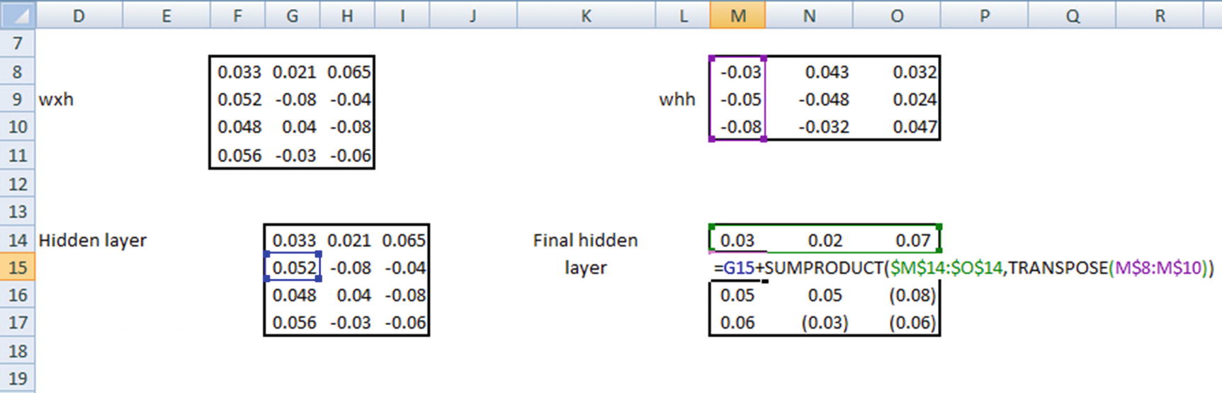
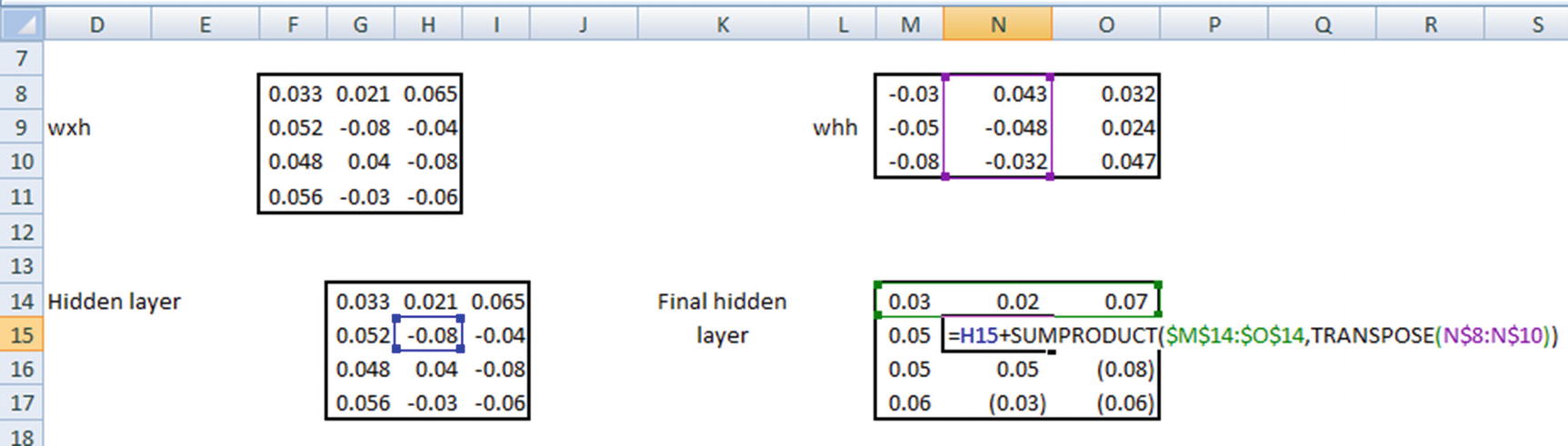
Time Step 3

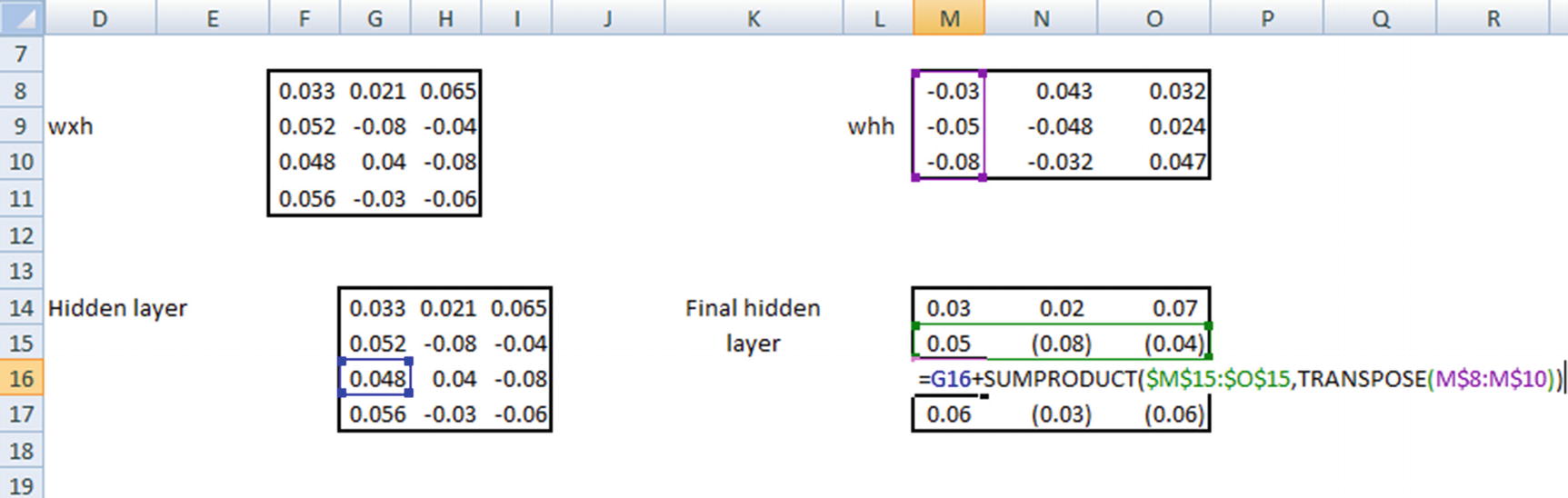
Similarly, at the third time step, the inputs would be the input at the current time step and the hidden unit values coming from the previous time step. Note that the hidden unit in the previous time step (t-1) is influenced by the hidden values coming from (t-2) also.

../images/463052_1_En_10_Chapter/463052_1_En_10_Figi_HTML.jpg

Similarly, the hidden layer values are calculated at the fourth time step.

Now that we have our hidden layer calculated, we pass it through an activation, just as we did it in traditional NN:

../images/463052_1_En_10_Chapter/463052_1_En_10_Figj_HTML.jpg

Given that the output from hidden layer activation is 1 × 3 in size for each input, in order to get an output of 1 × 4 in size (as the one-hot-encoded version of the expected output “example” is 4 columns in size), the hidden layer why should be 3 × 4 in dimension:

../images/463052_1_En_10_Chapter/463052_1_En_10_Figk_HTML.jpg

From the intermediate output, we perform the softmax activation as follows:

../images/463052_1_En_10_Chapter/463052_1_En_10_Figl_HTML.jpg

The second step of softmax would be to normalize each cell value to obtain a probability value:

../images/463052_1_En_10_Chapter/463052_1_En_10_Figm_HTML.jpg

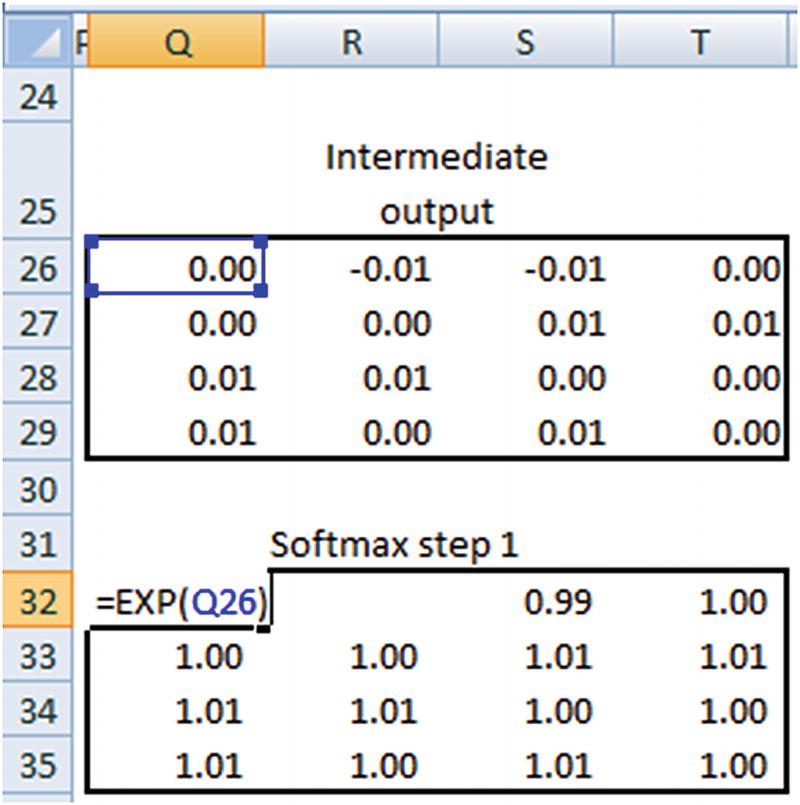
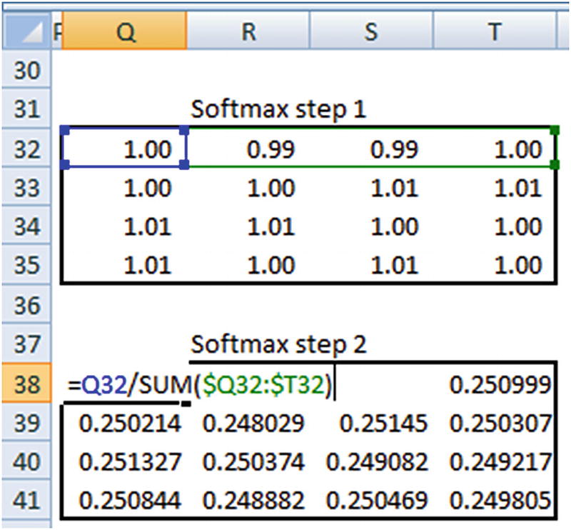
Once the probabilities are obtained, the loss is calculated by taking the cross entropy loss between the prediction and actual output.

Finally, we will be minimizing the loss through the combination of forward and backward propagation epochs in a similar manner as that of NN.

Implementing RNN: SimpleRNN

To see how RNN is implemented in keras, let’s go through a simplistic example (only to understand the keras implementation of RNN and then to solidify our understanding by implementing in Excel): classifying two sentences (which have an exhaustive list of three words). Through this toy example, we should be in a better position to understand the outputs quickly (code available as “simpleRNN.ipynb” in github):

from keras.preprocessing.text import one_hot

from keras.preprocessing.sequence import pad_sequences

from keras.models import Sequential

from keras.layers import Dense

from keras.layers import Flatten

from keras.layers.recurrent import SimpleRNN

from keras.layers.embeddings import Embedding

from keras.layers import LSTM

import numpy as np

Initialize the documents and encode the words corresponding to those documents :

# define documents

docs = ['very good',

'very bad']

# define class labels

labels = [1,0]

from collections import Counter

counts = Counter()

for i,review in enumerate(docs):

counts.update(review.split())

words = sorted(counts, key=counts.get, reverse=True)

vocab_size=len(words)

word_to_int = {word: i for i, word in enumerate(words, 1)}

encoded_docs = []

for doc in docs:

encoded_docs.append([word_to_int[word] for word in doc.split()])

Pad the documents to a maximum length of two words—this is to maintain consistency so that all the inputs are of the same size :

# pad documents to a max length of 2 words

max_length = 2

padded_docs = pad_sequences(encoded_docs, maxlen=max_length, padding="pre")

print(padded_docs)

../images/463052_1_En_10_Chapter/463052_1_En_10_Fign_HTML.jpg

Compiling a Model

The input shape to the SimpleRNN function should be of the form (number of time steps, number of features per time step). Also, in general RNN uses tanh as the activation function. The following code specifies the input shape as (2,1) because each input is based on two time steps and each time step has only one column representing it. unroll=True indicates that we are considering previous time steps :

# define the model

embed_length=1

max_length=2

model = Sequential()

model.add(SimpleRNN(1,activation='tanh', return_sequences=False,recurrent_initializer='Zeros',input_shape=(max_length,embed_length),unroll=True))

model.add(Dense(1, activation="sigmoid"))

# compile the model

model.compile(optimizer='adam', loss="binary_crossentropy", metrics=['acc'])

# summarize the model

print(model.summary())

SimpleRNN(1,) indicates that there is a neuron in the hidden layer. return_sequences is false because we are not returning any sequence of outputs, and it is a single output :

../images/463052_1_En_10_Chapter/463052_1_En_10_Figo_HTML.jpg

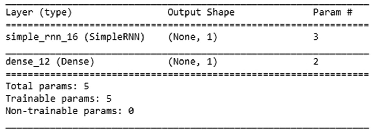
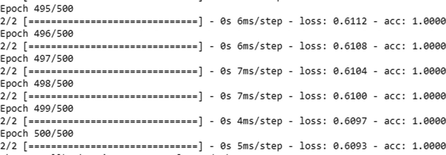
Once the model is compiled, let’s go ahead and fit the model , as follows:

model.fit(padded_docs.reshape(2,2,1),np.array(labels).reshape(max_length,1),epochs=500)

../images/463052_1_En_10_Chapter/463052_1_En_10_Figp_HTML.jpg

Note that we have reshaped padded_docs. That’s because we need to convert our training dataset into a format as follows while fitting: {data size, number of time steps, features per time step}. Also, labels should be in an array format, since the final dense layer in the compiled model expects an array.

Verifying the Output of RNN

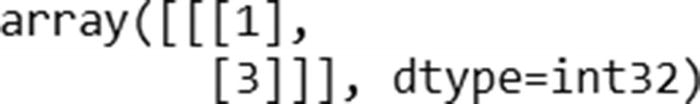
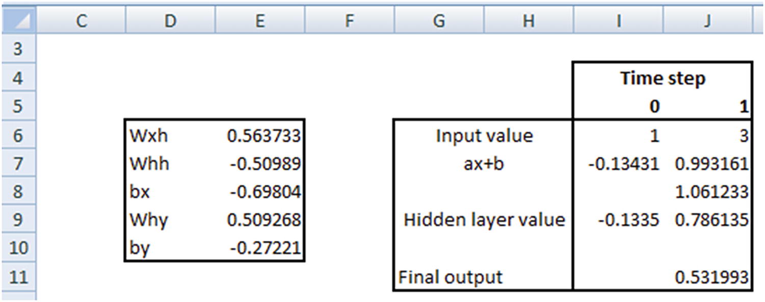
Now that we have fit our toy model, let’s verify the Excel calculations we created earlier. Note that we have taken the input to be the raw encodings {1,2,3}—in practice we would never take the raw encodings as they are, but would one-hot-encode or create embeddings for the input. We are taking the raw inputs as they are in this section only to compare the outputs from keras and the hand calculations we are going to do in Excel.

model.layers specifies the layers in the model, and weights gives us an understanding of the layers associated with the model:

../images/463052_1_En_10_Chapter/463052_1_En_10_Figq_HTML.jpg

model.weights gives us an indication of the names associated with the weights in the model:

../images/463052_1_En_10_Chapter/463052_1_En_10_Figr_HTML.jpg

model.get_weights() gives us the actual values of weights associated with the model:

../images/463052_1_En_10_Chapter/463052_1_En_10_Figs_HTML.jpg

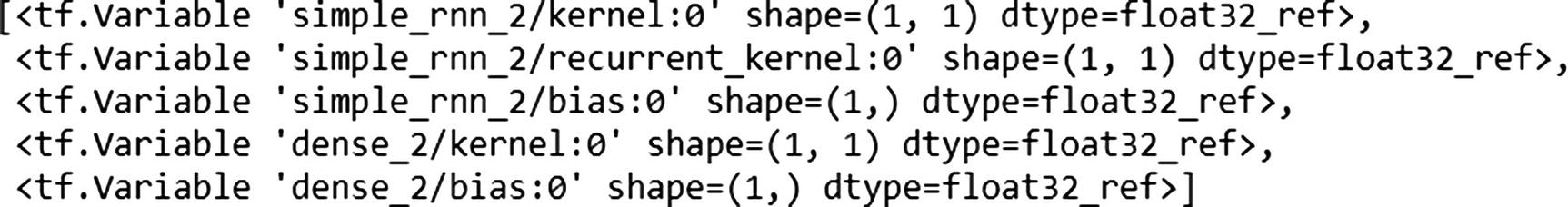
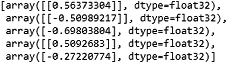
Note that the weights are ordered—that is, the first weight value corresponds to kernel:0. In other words, it is the same as wxh, which is the weight associated with the inputs.

recurrent_kernel:0 is the same as whh, which is the weight associated with the connection between the previous hidden layer earlier and the current time step’s hidden layer. bias:0 is the bias associated with the inputs. dense_2/kernel:0 is why—that is, the weight connecting the hidden layer to the output. dense_2/bias:0 is the bias associated with connection between the hidden layer and the output.

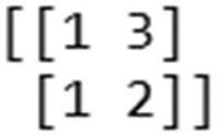
Let’s verify the prediction for the input [1,3]:

padded_docs[0].reshape(1,2,1)

../images/463052_1_En_10_Chapter/463052_1_En_10_Figt_HTML.jpg

import numpy as np

model.predict(padded_docs[0].reshape(1,2,1))

../images/463052_1_En_10_Chapter/463052_1_En_10_Figu_HTML.jpg

Given that the prediction is 0.53199 for the inputs [1,3] (in that order), let’s verify the same in Excel (available as “simple RNN working verification.xlsx” in github):

../images/463052_1_En_10_Chapter/463052_1_En_10_Figv_HTML.jpg

The input value at the two time steps are as follows:

../images/463052_1_En_10_Chapter/463052_1_En_10_Figw_HTML.jpg

The matrix multiplication between inputs and weights is calculated as follows:

../images/463052_1_En_10_Chapter/463052_1_En_10_Figx_HTML.jpg

Now that the matrix multiplication is done, we will go ahead and calculate the hidden layer value in time step 0:

../images/463052_1_En_10_Chapter/463052_1_En_10_Figy_HTML.jpg

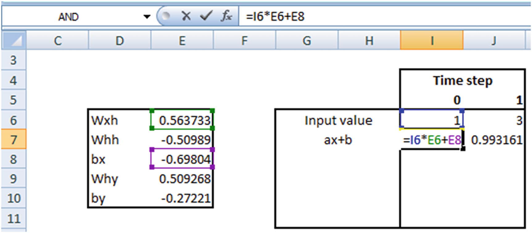
The hidden layer value in time step 1 is going to be the following:

tanh(Hidden layer value in time step 1 × Weight associated with hidden layer to hidden layer connection (whh) + Previous hidden layer value)

Let’s calculate the inner part of the tanh function first:

../images/463052_1_En_10_Chapter/463052_1_En_10_Figz_HTML.jpg

Now we’ll calculate the final hidden layer value of time step 1:

../images/463052_1_En_10_Chapter/463052_1_En_10_Figaa_HTML.jpg

Once the final hidden layer value is calculated, it is passed through a sigmoid layer, so the final output is calculated as follows:

../images/463052_1_En_10_Chapter/463052_1_En_10_Figab_HTML.jpg

The final output that we have from Excel is the same as what we got from keras as output and thus is a verification of the formulas that we looked at earlier:

../images/463052_1_En_10_Chapter/463052_1_En_10_Figac_HTML.jpg

Implementing RNN: Text Generation

Now that we’ve seen how a typical RNN works, let’s look into how to generate text using APIs provided by keras for RNN (available as “RNN text generation.ipynb” in github).

For this example, we will be working on the alice dataset ( www.gutenberg.org/ebooks/11 ):

1.
Import the packages:

from keras.models import Sequential
from keras.layers import Dense,Activation
from keras.layers.recurrent import SimpleRNN
import numpy as np
2.
Read the dataset:

fin=open('/home/akishore/alice.txt',encoding='utf-8-sig')
lines=[]
for line in fin:
  line = line.strip().lower()
  line = line.decode("ascii","ignore")
  if(len(line)==0):
    continue
  lines.append(line)
fin.close()
text = " ".join(lines)
3.
Normalize the file to have only small case and remove punctuation, if any:

text[:100]

# Remove punctuations in dataset
import re
text = text.lower()
text = re.sub('[^0-9a-zA-Z]+',' ',text)
4.
One-hot-encode the words:

from collections import Counter
counts = Counter()
counts.update(text.split())
words = sorted(counts, key=counts.get, reverse=True)
chars = words
total_chars = len(set(chars))
nb_chars = len(text.split())
char2index = {word: i for i, word in enumerate(chars)}
index2char = {i: word for i, word in enumerate(chars)}
5.
Create the input and target datasets :

SEQLEN = 10
STEP = 1
input_chars = []
label_chars = []
text2=text.split()
for i in range(0,nb_chars-SEQLEN,STEP):
    x=text2[i:(i+SEQLEN)]
    y=text2[i+SEQLEN]
    input_chars.append(x)
    label_chars.append(y)
print(input_chars[0])
print(label_chars[0])
6.
Encode the input and output datasets:

X = np.zeros((len(input_chars), SEQLEN, total_chars), dtype=np.bool)
y = np.zeros((len(input_chars), total_chars), dtype=np.bool)
# Create encoded vectors for the input and output values
for i, input_char in enumerate(input_chars):
    for j, ch in enumerate(input_char):
        X[i, j, char2index[ch]] = 1
    y[i,char2index[label_chars[i]]]=1
print(X.shape)
print(y.shape)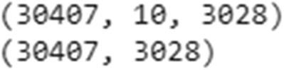

Note that, the shape of X indicates that we have a total 30,407 rows that have 10 words each, where each of the 10 words is expressed in a 3,028-dimensional space (since there are a total of 3,028 unique words).
7.
Build the model:

HIDDEN_SIZE = 128
BATCH_SIZE = 128
NUM_ITERATIONS = 100
NUM_EPOCHS_PER_ITERATION = 1
NUM_PREDS_PER_EPOCH = 100
model = Sequential()
model.add(SimpleRNN(HIDDEN_SIZE,return_sequences=False,input_shape=(SEQLEN,total_chars),unroll=True))
model.add(Dense(nb_chars, activation="sigmoid"))
model.compile(optimizer='rmsprop', loss="categorical_crossentropy")
model.summary()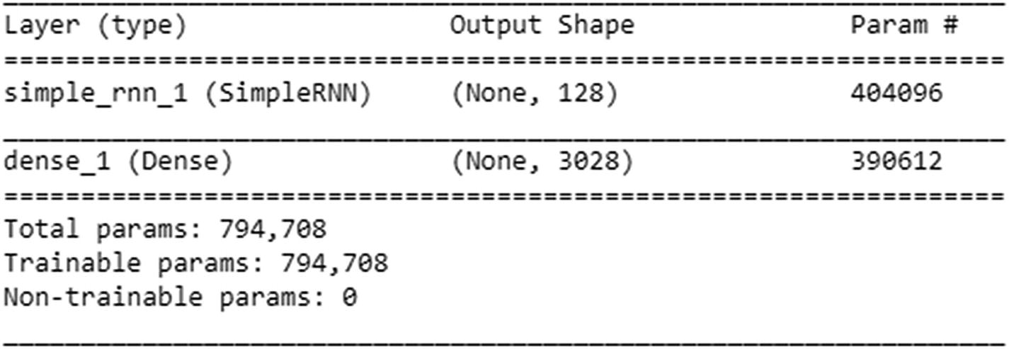
8.
Run the model, where we randomly generate a seed text and try to predict the next word given the set of seed words:

for iteration in range(150):
    print("=" * 50)
    print("Iteration #: %d" % (iteration))
    # Fitting the values
    model.fit(X, y, batch_size=BATCH_SIZE, epochs=NUM_EPOCHS_PER_ITERATION)
    # Time to see how our predictions fare
    # We are creating a test set from a random location in our dataset
    # In the code below, we are selecting a random input as our seed value of words
    test_idx = np.random.randint(len(input_chars))
    test_chars = input_chars[test_idx]
    print("Generating from seed: %s" % (test_chars))
    print(test_chars)
    # From the seed words, we are tasked to predict the next words
    # In the code below, we are predicting the next 100 words (NUM_PREDS_PER_EPOCH) after the seed words
    for i in range(NUM_PREDS_PER_EPOCH):
        # Pre processing the input data, just like the way we did before training the model
        Xtest = np.zeros((1, SEQLEN, total_chars))
        for i, ch in enumerate(test_chars):
            Xtest[0, i, char2index[ch]] = 1
        # Predict the next word
        pred = model.predict(Xtest, verbose=0)[0]
        # Given that, the predictions are probability values, we take the argmax to fetch the location of highest probability
        # Extract the word belonging to argmax
        ypred = index2char[np.argmax(pred)]
        print(ypred,end=' ')
        # move forward with test_chars + ypred so that we use the original 9 words + prediction for the next prediction
        test_chars = test_chars[1:] + [ypred]

The output in the initial iterations is just the single word the—always!

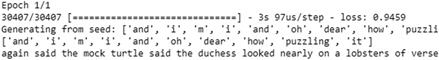
The output at the end of 150 iterations is as follows (note that the below is only a partial output):

../images/463052_1_En_10_Chapter/463052_1_En_10_Figah_HTML.jpg

The preceding output has very little loss. And if you look at the output carefully after you execute code, after some iterations it is reproducing the exact text that is present in the dataset—a potential overfitting issue. Also, notice the shape of our input: ~30K inputs, where there are 3,028 columns. Given the low ratio of rows to columns, there is a chance of overfitting. This is likely to work better as the number of input samples increases a lot more.

The issue of having a high number of columns can be overcome by using embedding, which is very similar to the way in which we calculated word vectors. Essentially, embeddings represent a word in a much lower dimensional space.

Embedding Layer in RNN

To see how embedding works, let’s look at a dataset that tries to predict customer sentiment of an airline based on customer tweets (code available as “RNNsentiment.ipynb” in github):

1.
As always, import the relevant packages :

#import relevant packages
from keras.layers import Dense, Activation
from keras.layers.recurrent import SimpleRNN
from keras.models import Sequential
from keras.utils import to_categorical
from keras.layers.embeddings import Embedding
from sklearn.cross_validation import train_test_split
import numpy as np
import nltk
from nltk.corpus import stopwords
import re
import pandas as pd
#Let us go ahead and read the dataset:
t=pd.read_csv('/home/akishore/airline_sentiment.csv')
t.head()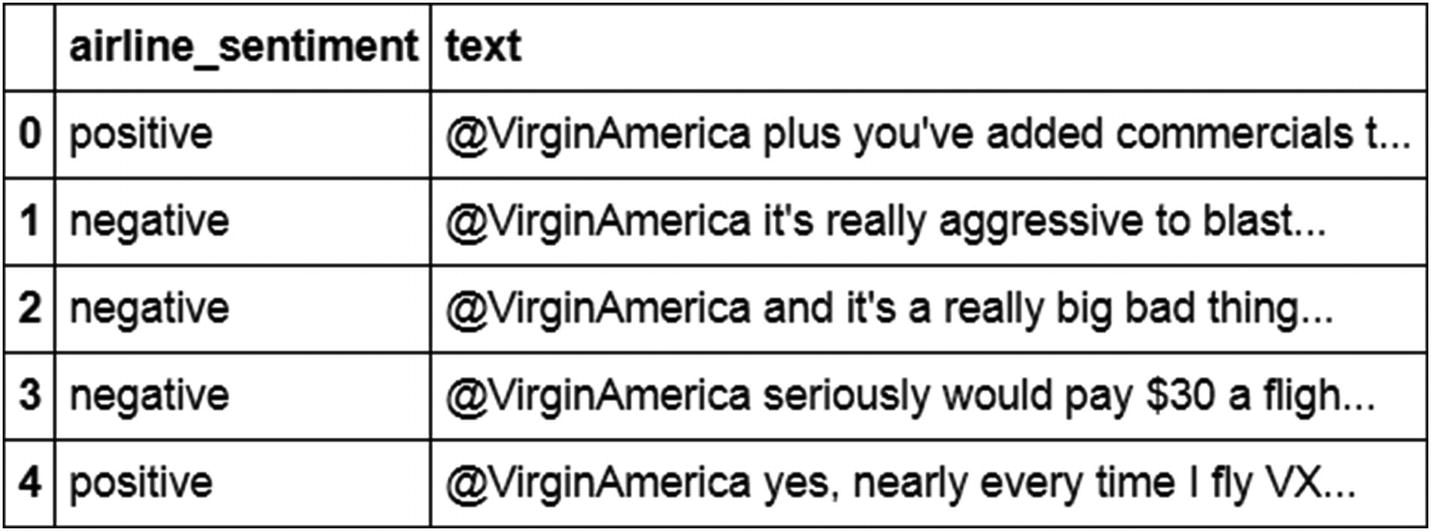

import numpy as np
t['sentiment']=np.where(t['airline_sentiment']=="positive",1,0)
2.
Given that the text is noisy, we will pre-process it by removing punctuation and also converting all words into lowercase :

def preprocess(text):
    text=text.lower()
    text=re.sub('[^0-9a-zA-Z]+',' ',text)
    words = text.split()
    #words2=[w for w in words if (w not in stop)]
    #words3=[ps.stem(w) for w in words]
    words4=' '.join(words)
    return(words4)
t['text'] = t['text'].apply(preprocess)
3.
Similar to how we developed in the previous section, we convert each word into an index value as follows:

from collections import Counter
counts = Counter()
for i,review in enumerate(t['text']):
counts.update(review.split())
words = sorted(counts, key=counts.get, reverse=True)
words[:10]

chars = words
nb_chars = len(words)
word_to_int = {word: i for i, word in enumerate(words, 1)}
int_to_word = {i: word for i, word in enumerate(words, 1)}
word_to_int['the']
#3
int_to_word[3]
#the
4.
Map each word in a review to its corresponding index :

mapped_reviews = []
for review in t['text']:
mapped_reviews.append([word_to_int[word] for word in review.split()])
t.loc[0:1]['text']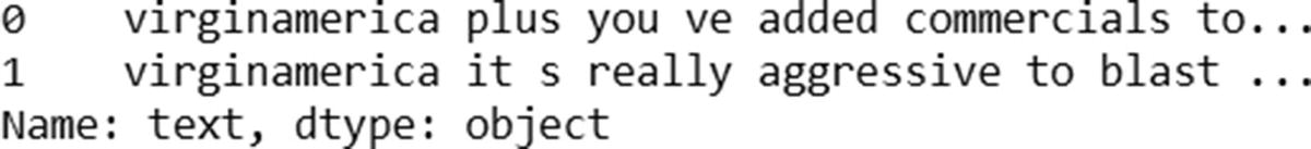

mapped_reviews[0:2]

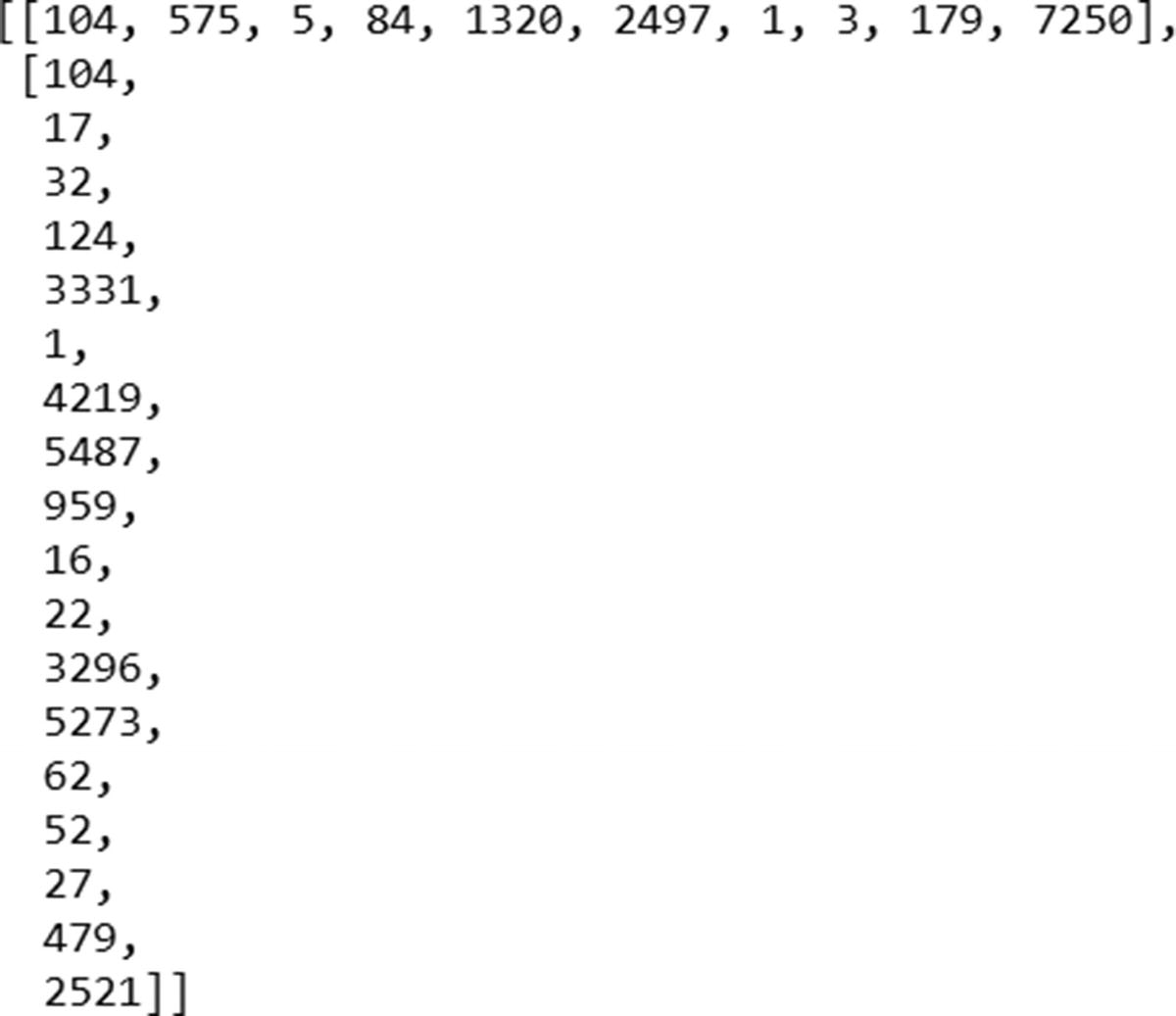
Note that, the index of virginamerica is the same in both reviews (104).
5.
Initialize a sequence of zeroes of length 200. Note that we have chosen 200 as the sequence length because no review has more than 200 words in it. Moreover, the second part of the following code makes sure that for all reviews that are less than 200 words in size, all the starting indices are zero padded and only the last indices are filled with index corresponding to the words present in the review:

sequence_length = 200
sequences = np.zeros((len(mapped_reviews), sequence_length),dtype=int)
for i, row in enumerate(mapped_reviews):
review_arr = np.array(row)
sequences[i, -len(row):] = review_arr[-sequence_length:]
6.
We further split the dataset into train and test datasets , as follows:

y=t['sentiment'].values
X_train, X_test, y_train, y_test = train_test_split(sequences, y, test_size=0.30,random_state=10)
y_train2 = to_categorical(y_train)
y_test2 = to_categorical(y_test)
7.
Once the datasets are in place, we go ahead and create our model, as follows. Note that embedding as a function takes in as input the total number of unique words, the reduced dimension in which we express a given word, and the number of words in an input:

top_words=12679
embedding_vecor_length=32
max_review_length=200
model = Sequential()
model.add(Embedding(top_words, embedding_vecor_length, input_length=max_review_length))
model.add(SimpleRNN(1, return_sequences=False,unroll=True))
model.add(Dense(2, activation="softmax"))
model.compile(loss='categorical_crossentropy', optimizer="adam", metrics=['accuracy'])
print(model.summary())
model.fit(X_train, y_train2, validation_data=(X_test, y_test2), epochs=50, batch_size=1024)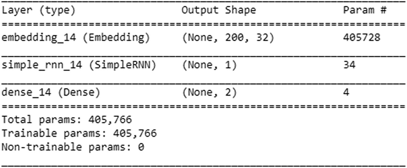

Now let’s look at the summary output of the preceding model. There are a total of 12,679 unique words in the dataset. The embedding layer ensures that we represent each of the words in a 32-dimensional space, hence the 405,728 parameters in the embedding layer.

Now that we have 32 embedded dimensional inputs, each input is now connected to one hidden layer unit—thus 32 weights. Along, with the 32 weights, we would have a bias. The final weight corresponding to this layer would be the weight that connects the previous hidden to unit value to the current hidden unit. Thus a total of 34 weights.

Note that, given that there is an output coming from the embedding layer, we don’t need to specify the input shape in the SimpleRNN layer. Once the model has run, the output classification accuracy turns out to be close to 87%.

Issues with Traditional RNN

A traditional RNN that takes multiple time steps into account for giving a prediction is shown in Figure 10-5.

../images/463052_1_En_10_Chapter/463052_1_En_10_Fig5_HTML.png — Figure 10-5
An RNN with multiple time steps

Note that as time step increases, the impact of input from a much earlier layer on output of later layers is much less. That can be seen in the following (for now, we’ll ignore the bias terms):

h₁ = Wx₁
h₂ = Wx₂ + Uh₁ = Wx₂ + UWx₁
h₃ = Wx₃ + Uh₂ = Wx₃ + UWx₂ + U²Wx₁
h₄ = Wx₄ + Uh₃ = Wx₄ + UWX₃ + U²WX₂ + U³WX₁
h₅ = Wx₅ + Uh₄ = Wx₅ + UWX₄ + U²WX₃ + U³WX₂ + U⁴WX₁

Note that as the time stamp increases, the value of the hidden layer is highly dependent on X₁ if U > 1, and a little dependent on X₁ if U < 1.

The Problem of Vanishing Gradient

The gradient of U⁴ with respect to U is 4 × U³. In such a case, note that if U < 1, the gradient is very small, so arriving at the ideal weights takes a very long time if the output at a much a later time step depends on the input at a given time step. This results in an issue when there is a dependency on a word that occurred much earlier in the time steps in some sentences. For example, “I am from India. I speak fluent ____.” In this case, if we did not take the first sentence into account, the output of the second sentence, “I speak fluent ____” could be the name of any language. Because we mentioned the country in the first sentence, we should be able to narrow things down to languages specific to India.

The Problem of Exploding Gradients

In the preceding scenario, if U > 1, then gradients increase by a much larger amount. This would result in having a very high weightage for inputs that occurred much earlier in the time steps and low weightage for inputs that occurred near the word that we are trying to predict.

Hence, depending on the value of U (weights of the hidden layer), the weights either get updated very quickly or take a very long time.

Given that vanishing/exploding gradient is an issue, we should deal with RNNs in a slightly different way.

LSTM

Long short-term memory (LSTM) is an architecture that helps overcome the vanishing or exploding gradient problem we saw earlier. In this section, we will look at the architecture of LSTM and see how it helps in overcoming the issue with traditional RNN.

LSTM is shown in Figure 10-6.

../images/463052_1_En_10_Chapter/463052_1_En_10_Fig6_HTML.png — Figure 10-6
LSTM

Note that although the input X and the output of the hidden layer (h) remain the same, the activations that happen within the hidden layer are different. Unlike the traditional RNN, which has tanh activation, there are different activations that happen within LSTM. We’ll go through each of them.

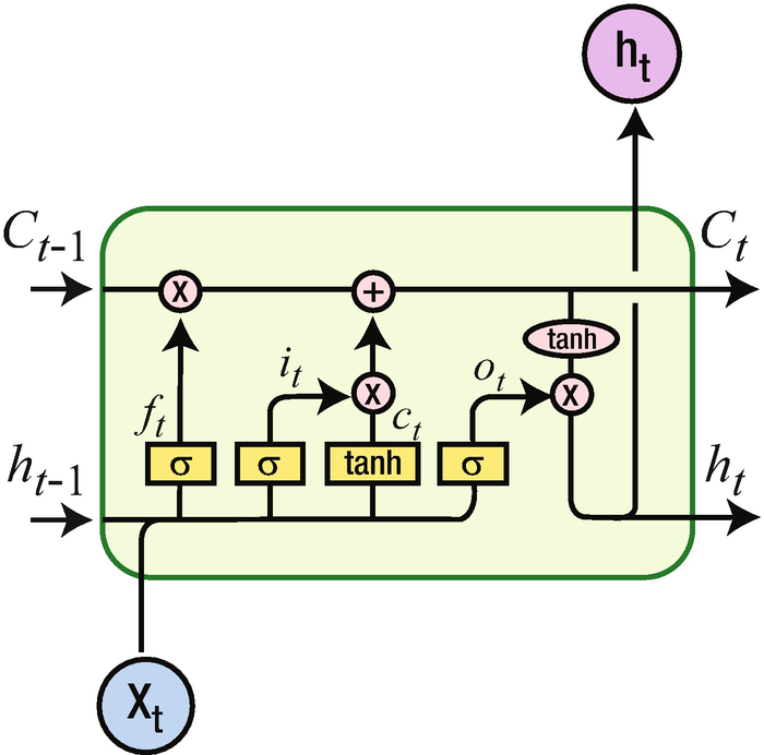
In Figure 10-7, X and h represent the input and hidden layer, as we saw earlier.

../images/463052_1_En_10_Chapter/463052_1_En_10_Fig7_HTML.png — Figure 10-7
Various components of LSTM

C represents the cell state. You can think of cell state as a way in which long-term dependencies are captured.

f represents the forget gate:

${f}_t=\sigma \left({W}_{xf}{x}^{(t)}+{W}_{hf}{h}^{\left(t-1\right)}+{b}_f\right)$

Note that the sigmoid gives us a mechanism to specify what needs to be forgotten. This way, some historical words that are captured in h^(t–1) are selectively forgotten.

Once we figure what needs to be forgotten, the cell state gets updated as follows:

${c}_t=\left({c}_{t-1}\otimes f\right)$

Note that ../images/463052_1_En_10_Chapter/463052_1_En_10_Figan_HTML.jpg represents element-to-element multiplication.

Consider that once we fill in the blank in “I live in India. I speak ____” with the name of an Indian language, we don’t need the context of “I live in India” anymore. This is where the forget gate helps in selectively forgetting the information that is not needed anymore.

Once we figure out what needs to be forgotten in the cell state, we can go ahead and update the cell state based on the current input.

In the next step, the input that needs to update the cell state is achieved through the sigmoid application on top of input, and the magnitude of update (either positive or negative) is obtained through the tanh activation.

The input can be specified as follows:

${i}_t=\sigma \left({W}_{xi}{x}^{(t)}+{W}_{hi}{h}^{\left(t-1\right)}+{b}_i\right)$

The modulation can be specified like this:

${g}_t=\tanh \left({W}_{xg}{x}^{(t)}+{W}_{hg}{h}^{\left(t-1\right)}+{b}_g\right)$

The cell state thus finally gets updated as the following:

${C}^{(t)}=\left({C}^{\left(t-1\right)}\odot {f}_t\right)\oplus \left({i}_t\odot {g}_t\right)$

In the final gate, we need to specify what part of the combination of input and cell state needs to be outputted to the next hidden layer:

${o}_t=\sigma \left({W}_{xo}{x}^{(t)}+{W}_{ho}{h}^{\left(t-1\right)}+{b}_o\right)$

The final hidden layer is represented like this:

${h}^{(t)}={o}_t\odot \tanh \left({C}^{(t)}\right)$

Given that the cell state can memorize the values that are needed at a later point in time, LSTM provides better results than traditional RNN in predicting the next word, typically in sentiment classification. This is especially useful in a scenario where there is a long-term dependency that needs to be taken care of.

Implementing Basic LSTM in keras

To see how the theory presented so far translates into action, let’s relook at the toy example we saw earlier (code available as “LSTM toy example.ipynb” in github):

1.
Import the relevant packages :

from keras.preprocessing.text import one_hot
from keras.preprocessing.sequence import pad_sequences
from keras.models import Sequential
from keras.layers import Dense
from keras.layers import Flatten
from keras.layers.recurrent import SimpleRNN
from keras.layers.embeddings import Embedding
from keras.layers import LSTM
import numpy as np
2.
Define documents and labels :

# define documents
docs = ['very good',
'very bad']
# define class labels
labels = [1,0]
3.
One-hot-encode the documents:

from collections import Counter
counts = Counter()
for i,review in enumerate(docs):
counts.update(review.split())
words = sorted(counts, key=counts.get, reverse=True)
vocab_size=len(words)
word_to_int = {word: i for i, word in enumerate(words, 1)}
encoded_docs = []
for doc in docs:
encoded_docs.append([word_to_int[word] for word in doc.split()])
encoded_docs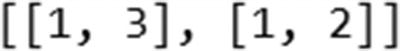
4.
Pad documents to a maximum length of two words :

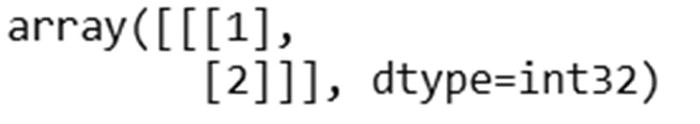
max_length = 2
padded_docs = pad_sequences(encoded_docs, maxlen=max_length, padding="pre")
print(padded_docs)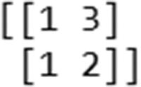
5.
Build the model :

model = Sequential()
model.add(LSTM(1,activation='tanh', return_sequences=False,recurrent_initializer='Zeros',recurrent_activation='sigmoid',
input_shape=(2,1),unroll=True))
model.add(Dense(1, activation="sigmoid"))
model.compile(optimizer='adam', loss="binary_crossentropy", metrics=['acc'])
print(model.summary())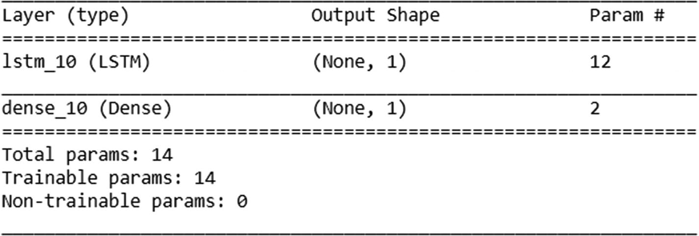

Note that in the preceding code , we have initialized the recurrent initializer and recurrent activation to certain values only to make this toy example easier to understand when implemented in Excel. The purpose is to help you understand what is happening in the back end only.

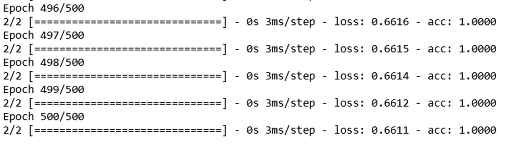
Once the model is initialized as discussed, let’s go ahead and fit the model:

model.fit(padded_docs.reshape(2,2,1),np.array(labels).reshape(max_length,1),epochs=500)

../images/463052_1_En_10_Chapter/463052_1_En_10_Figar_HTML.jpg

The layers of this model are as follows. Here is model.layers :

../images/463052_1_En_10_Chapter/463052_1_En_10_Figas_HTML.jpg

The weights and the order of weights can be obtained as follows:

model.layers[0].get_weights()

../images/463052_1_En_10_Chapter/463052_1_En_10_Figat_HTML.jpg

model.layers[0].trainable_weights

../images/463052_1_En_10_Chapter/463052_1_En_10_Figau_HTML.jpg

model.layers[1].get_weights()

../images/463052_1_En_10_Chapter/463052_1_En_10_Figav_HTML.jpg

model.layers[1].trainable_weights

../images/463052_1_En_10_Chapter/463052_1_En_10_Figaw_HTML.jpg

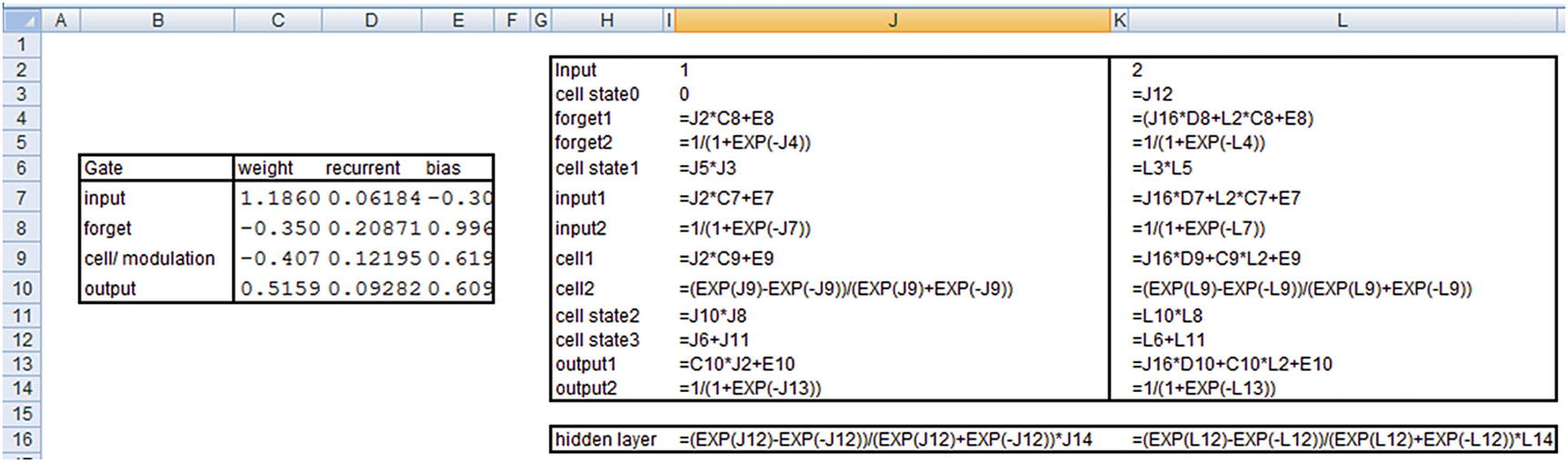
From the preceding code , we can see that weights of input (kernel) are obtained first, followed by weights corresponding to the hidden layer (recurrent_kernel) and finally the bias in the LSTM layer.

Similarly, in the dense layer (the layer connecting the hidden layer to output), the weight to be multiplied with the hidden layer comes first, followed by the bias.

Also note that the order in which weights and bias appear in the LSTM layer is as follows:

1.
Input gate
2.
Forget gate
3.
Modulation gate (cell gate)
4.
Output gate

Now that we have our outputs, let’s go ahead and calculate the predictions for input. Note that just like in the previous section, we are using raw encoded inputs (1,2,3) without further processing them—only to see how the calculation works.

In practice, we would be further processing the inputs, potentially encoding them into vectors to obtain the predictions, but in this example we are interested in solidifying our knowledge of how LSTM works by replicating the predictions from LSTM in Excel :

padded_docs[1].reshape(1,2,1)

../images/463052_1_En_10_Chapter/463052_1_En_10_Figax_HTML.jpg

model.predict(padded_docs[1].reshape(1,2,1))

../images/463052_1_En_10_Chapter/463052_1_En_10_Figay_HTML.jpg

Now that we have a predicted probability of 0.4485 from the model, let’s hand-calculate the values in Excel (available in github as “LSTM working details.xlsx”):

../images/463052_1_En_10_Chapter/463052_1_En_10_Figaz_HTML.jpg

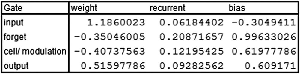
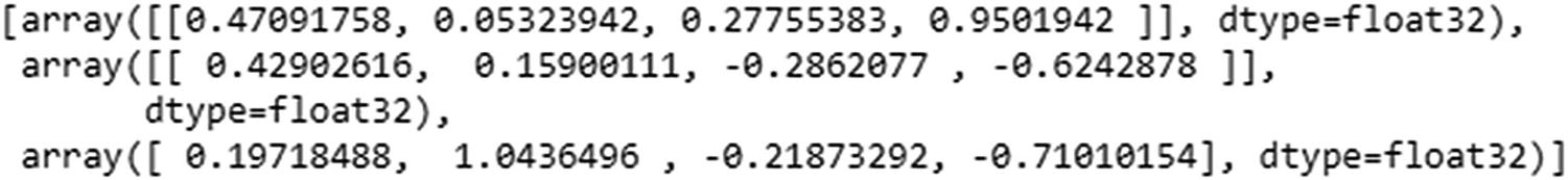
Note that the values here are taken from keras’s model.layers[0].get_weights() output.

Before proceeding with the calculation of the values at various gates, note that we have initialized the value of recurrent layer (h_t-1) to 0. In the first time step, the input is a value of 1. Let’s calculate the value at various gates:

../images/463052_1_En_10_Chapter/463052_1_En_10_Figba_HTML.jpg

The calculations to obtain the preceding output are as follows:

../images/463052_1_En_10_Chapter/463052_1_En_10_Figbb_HTML.jpg

Now that all the values at various gates are calculated, we’ll calculate the output (the hidden layer):

../images/463052_1_En_10_Chapter/463052_1_En_10_Figbc_HTML.jpg

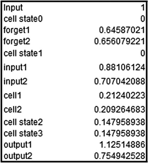
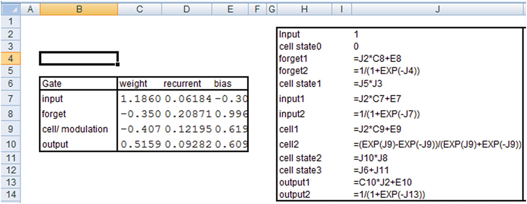
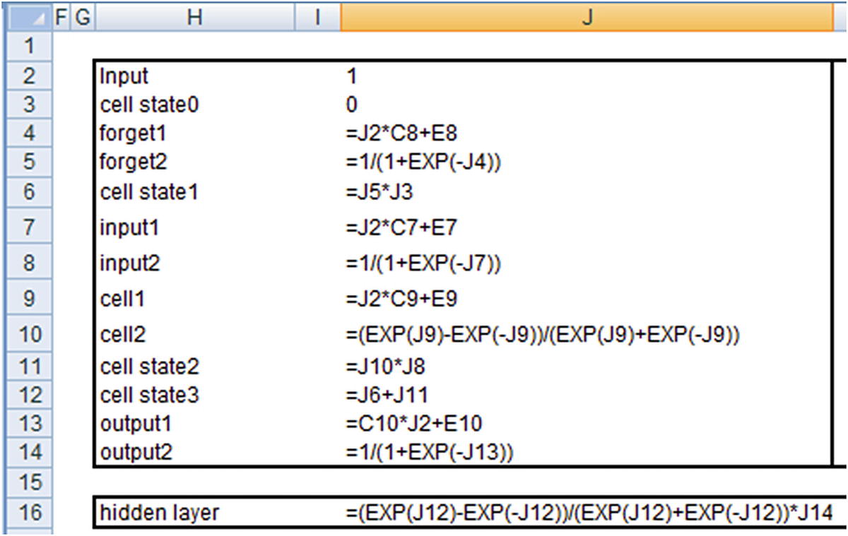
The hidden layer value just shown is the hidden layer output at the time step where the input is 1.

Now, we’ll go ahead and calculate the hidden layer value when the input is 2 (which is the input at the second time step of our data point that we were predicting in the code earlier):

../images/463052_1_En_10_Chapter/463052_1_En_10_Figbd_HTML.jpg

Let’s see how the values are obtained for the various gates and the hidden layer for the second input . The key to note here is that the hidden layer of the first time step output is an input to the calculation of all gates in the second input:

../images/463052_1_En_10_Chapter/463052_1_En_10_Figbe_HTML.jpg

Finally, given that we have calculated the hidden layer output of the second time step, we calculate the output, as follows:

../images/463052_1_En_10_Chapter/463052_1_En_10_Figbf_HTML.jpg

The final output of the preceding calculations is shown here:

../images/463052_1_En_10_Chapter/463052_1_En_10_Figbg_HTML.jpg

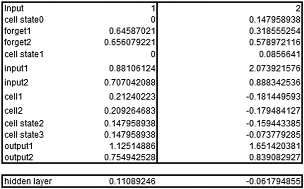
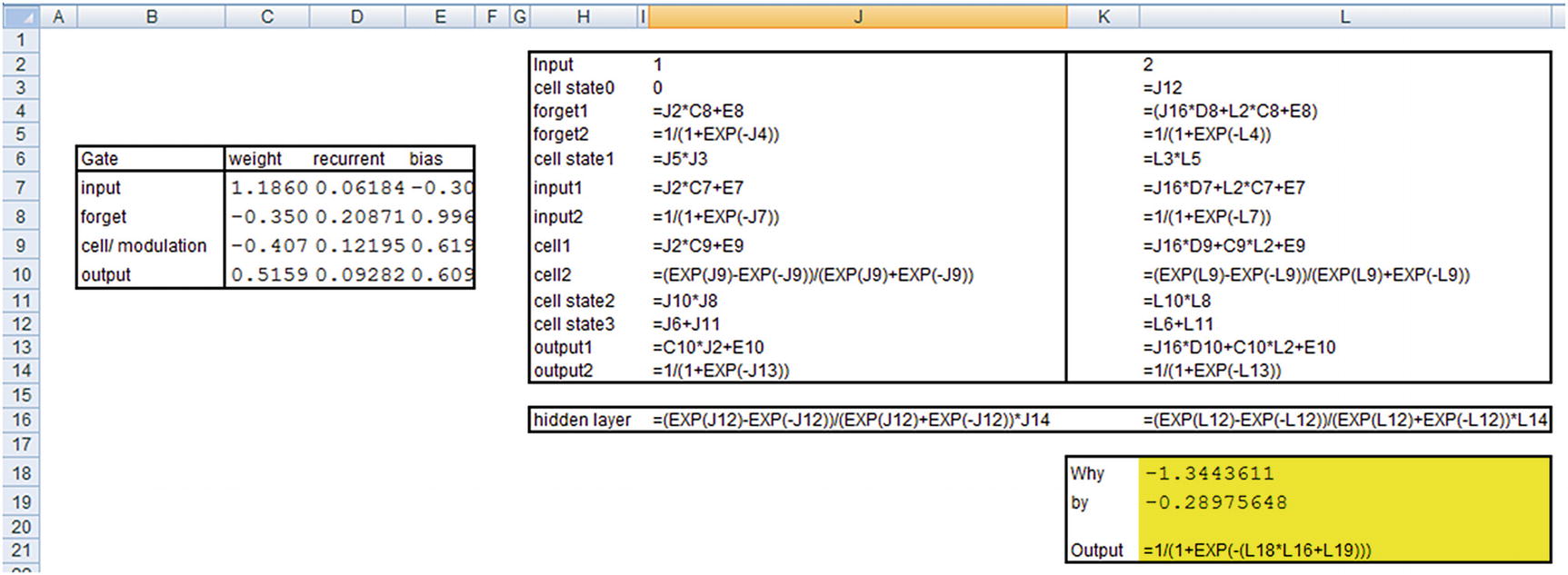
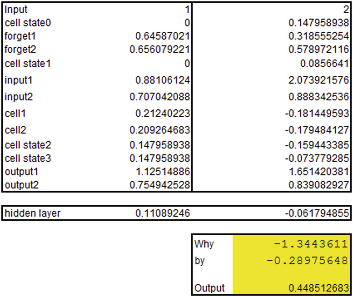
Note that the output that we’ve derived is the same as what we see in the keras output .

Implementing LSTM for Sentiment Classification

In the last section, we implemented sentiment classification using RNN in keras. In this section, we will look at implementing the same using LSTM. The only change in the code we saw above will be the model compiling part, where we will be using LSTM in place of SimpleRNN—everything else will remain the same (code is available in “RNN sentiment.ipynb” file in github):

top_words=nb_chars

embedding_vecor_length=32

max_review_length=200

model = Sequential()

model.add(Embedding(top_words, embedding_vecor_length, input_length=max_review_length))

model.add(LSTM(10))

model.add(Dense(2, activation="softmax"))

model.compile(loss='categorical_crossentropy', optimizer="adam", metrics=['accuracy'])

print(model.summary())

model.fit(X_train, y_train2, validation_data=(X_test, y_test2), epochs=50, batch_size=1024)

Once you implement the model, you should see that the prediction accuracy of LSTM is slightly better than that of RNN. In practice, for the dataset we looked earlier, LSTM gives an accuracy of 91%, whereas RNN gave an accuracy of 87%. This can be further fine-tuned by adjusting various hyper-parameters that are provided by the functions.

Implementing RNN in R

To look at how to implement RNN/LSTM in R, we will use the IMDB sentiment classification dataset that comes pre-built along with the kerasR package (code available as “kerasR_code_RNN.r” in github):

# Load the dataset

library(kerasR)

imdb <- load_imdb(num_words = 500, maxlen = 100)

Note that we are fetching only the top 500 words by specifying num_words as a parameter. We are also fetching only those IMDB reviews that have a length of at most 100 words.

Let’s explore the structure of the dataset:

str(imdb)

We should notice that in the pre-built IMDB dataset that came along with the kerasR package, each word is replaced by the index it represents by default. So we do not have to perform the step of word-to-index mapping:

# Build the model with an LSTM

model <- Sequential()

model$add(Embedding(500, 32, input_length = 100, input_shape = c(100)))

model$add(LSTM(32)) # Use SimpleRNN, if we were to perform a RNN function

model$add(Dense(256))

model$add(Activation('relu'))

model$add(Dense(1))

model$add(Activation('sigmoid'))

# Compile and fit the model

keras_compile(model, loss = 'binary_crossentropy', optimizer = Adam(),metrics='binary_accuracy')

keras_fit(model, X_train, Y_train, batch_size = 1024, epochs = 50, verbose = 1,validation_data = list(X_test,Y_test))

The preceding results in close to 79% accuracy on the test dataset prediction .

Summary

In this chapter, you learned the following:

RNNs are extremely helpful in dealing with data that has time dependency.
RNNs face issues with vanishing or exploding gradient when dealing with long-term dependency in data.
LSTM and other recent architectures come in handy in such a scenario.
LSTM works by storing the information in cell state, forgetting the information that does not help anymore, selecting the information as well as the amount of information that need to be added to cell state based on current input, and finally, the information that needs to be outputted to the next state.

Previous Chapter

9. Convolutional Neural Network

Next Chapter

11. Clustering

Table of Contents for Pro Machine Learning Algorithms : A Hands-On Approach to Implementing Algorithms in Python and R