Minimizing the effort of users to search for a product
Reminding users about sessions they closed earlier
Helping users discover more products
Recommender widgets in e-commerce websites
Recommended items sent to email addresses
Recommendations of friends/contacts in social network sites
Identify similar products to the products they are viewing
Know whether the product is fairly priced
Find accessories or complementary products
That’s why recommender systems often boost sales by a considerable amount.
- To predict the rating a user would give (or likelihood a user would purchase) an item using
Collaborative filtering
Matrix factorization
Euclidian and cosine similarity measures
How to implement recommendation algorithms in Excel, Python, and R
A recommender system is almost like a friend. It infers your preferences and provides you with options that are personalized to you. There are multiple ways of building a recommender system, but the goal is for it to be a way of relating the user to a set of other users, a way of relating an item to a set of other items, or a combination of both.
Given that recommending is about relating one user/item to another, it translates to a problem of k-nearest neighbors: identifying the few that are very similar and then basing a prediction based on the preferences exhibited by the majority of nearest neighbors.
Understanding k-nearest Neighbors
A nearest neighbor is the entity (a data point, in the case of a dataset) that is closest to the entity under consideration. Two entities are close if the distance between them is small.
User | Weight |
|---|---|
A | 60 |
B | 62 |
C | 90 |
We can intuitively conclude that users A and B are more similar to each other in terms of weight when compared to C.
User | Weight | Age |
|---|---|---|
A | 60 | 30 |
B | 62 | 35 |
C | 90 | 30 |
The “distance” between user A and B can be measured as:

This kind of distance between users is calculated similarly to the way the distance between two points is calculated.
Car model | Max speed attainable | No. of gears |
|---|---|---|
A | 100 | 4 |
B | 110 | 5 |
C | 100 | 5 |
In the preceding table, if we were measuring to see the similarity between cars using the traditional “distance” metric , we might conclude that models A and C are most similar to each other (even though their number of gears are different). Yet intuitively we know that B and C are more similar to each other than A and C, because they have identical number of gears and their max attainable speeds are similar.
The discrepancy highlights the issue of scale of variables, where one variable has a very high magnitude when compared to the other variable. To get around this issue, typically we would normalize the variables before proceeding further with distance calculations. Normalizing variables is a process of bringing all the variables to a uniform scale.
Divide each variable by the maximum value of the variable (bringing all the values between –1 and 1)
Find the Z-score of each data point of the variable. Z-score is (value of data point – mean of variable) / (standard deviation of the variable).
Divide each variable by the (maximum – minimum) value of the variable (called min max scaling).
Steps like these help normalize variables, thereby preventing the issues with scaling.
Once the distance of a data point to other data points is obtained—in the case of recommender systems, that is, once the nearest items to a given item are identified—the system will recommend these items to a user if it learns that the user has historically liked a majority of the nearest neighborhood items.
The k in k-nearest neighbors stands for the number of nearest neighbors to consider while taking a majority vote on whether the user likes the nearest neighbors or not. For example, if the user likes 9 out of 10 (k) nearest neighbors to an item, we’ll recommend the item to user. Similarly, if the user likes only 1 out of 10 nearest neighbors of the item, we’ll not recommend the item to user (because the liked items are in minority).
Neighborhood-based analysis takes into account the way in which multiple users can collaboratively help predict whether a user might like something or not.
With this background, we’ll move on and look at the evolution of recommender system algorithms.
Working Details of User-Based Collaborative Filtering
User-based refers, of course, to something based on users. Collaborative means using some relation (similarity) between users. And filtering refers to filtering out some users from all users.
User/ Movie | Just My Luck | Lady in the Water | Snakes on a Plane | Superman Returns | The Night Listener | You Me and Dupree |
|---|---|---|---|---|---|---|
Claudia Puig | 3 | 3.5 | 4 | 4.5 | 2.5 | |
Gene Seymour | 1.5 | 3 | 3.5 | 5 | 3 | 3.5 |
Jack Matthews | 3 | 4 | 5 | 3 | 3.5 | |
Lisa Rose | 3 | 2.5 | 3.5 | 3.5 | 3 | 2.5 |
Mick LaSalle | 2 | 3 | 4 | 3 | 3 | 2 |
Toby | 4.5 | 4 | 1 |
Euclidian distance between users
Cosine similarity between users
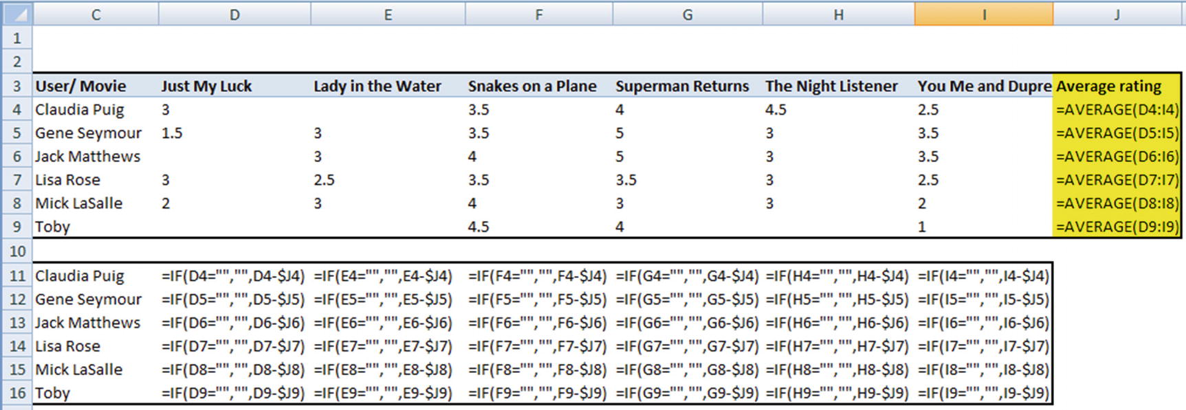
Euclidian Distance
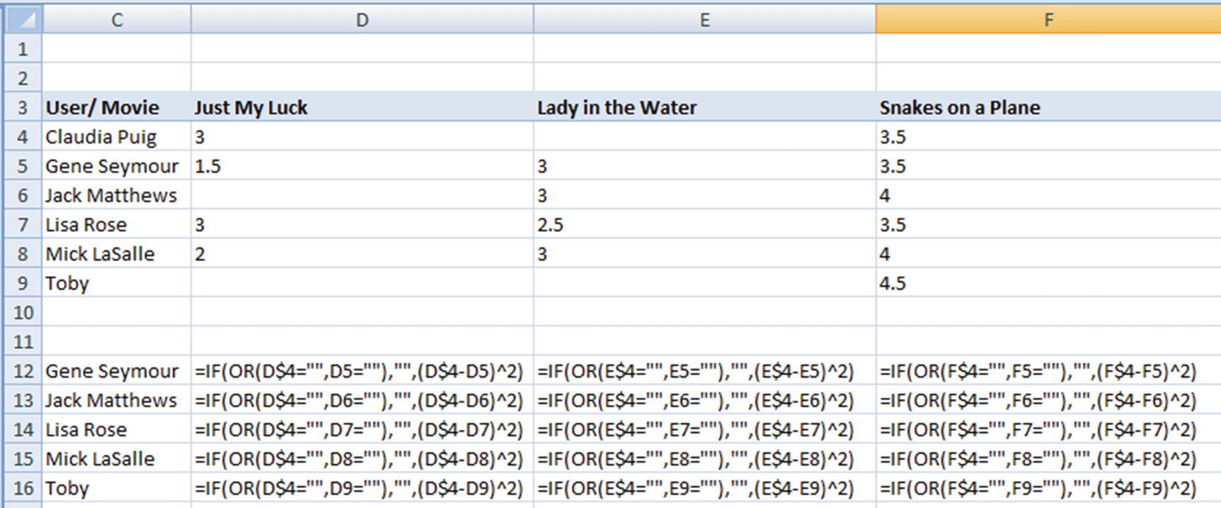
We aren’t seeing the complete picture due to space and formatting constraints, but essentially the same formula is applied across columns.
Note that the overall distance value is the average of all the distances where both users have rated a given movie. Given that Lisa Rose is the user who has the least overall distance with Claudia, we will consider the rating provided by Lisa as the rating that Claudia is likely to give to the movie Lady in the Water.
One major issue to be considered in such a calculation is that some users may be soft critics and some users may be harsher critics. Users A and B may have implicitly had similar experiences watching a given movie , but explicitly their ratings might be different.
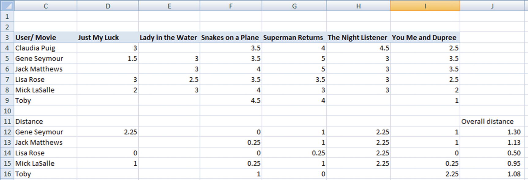
Normalizing for a User
Given that users differ in their levels of criticism, we need to make sure that we get around that problem. Normalization can help here.
- 1.
Take the average rating across all movies of a given user.
- 2.
Take the difference between each individual movie and the average rating of the user.
By taking the difference between a rating of an individual movie and the average rating of the user, we would know whether they liked a movie more than the average movie they watch, less than the average movie they watch, or equal to the average movie they watch.
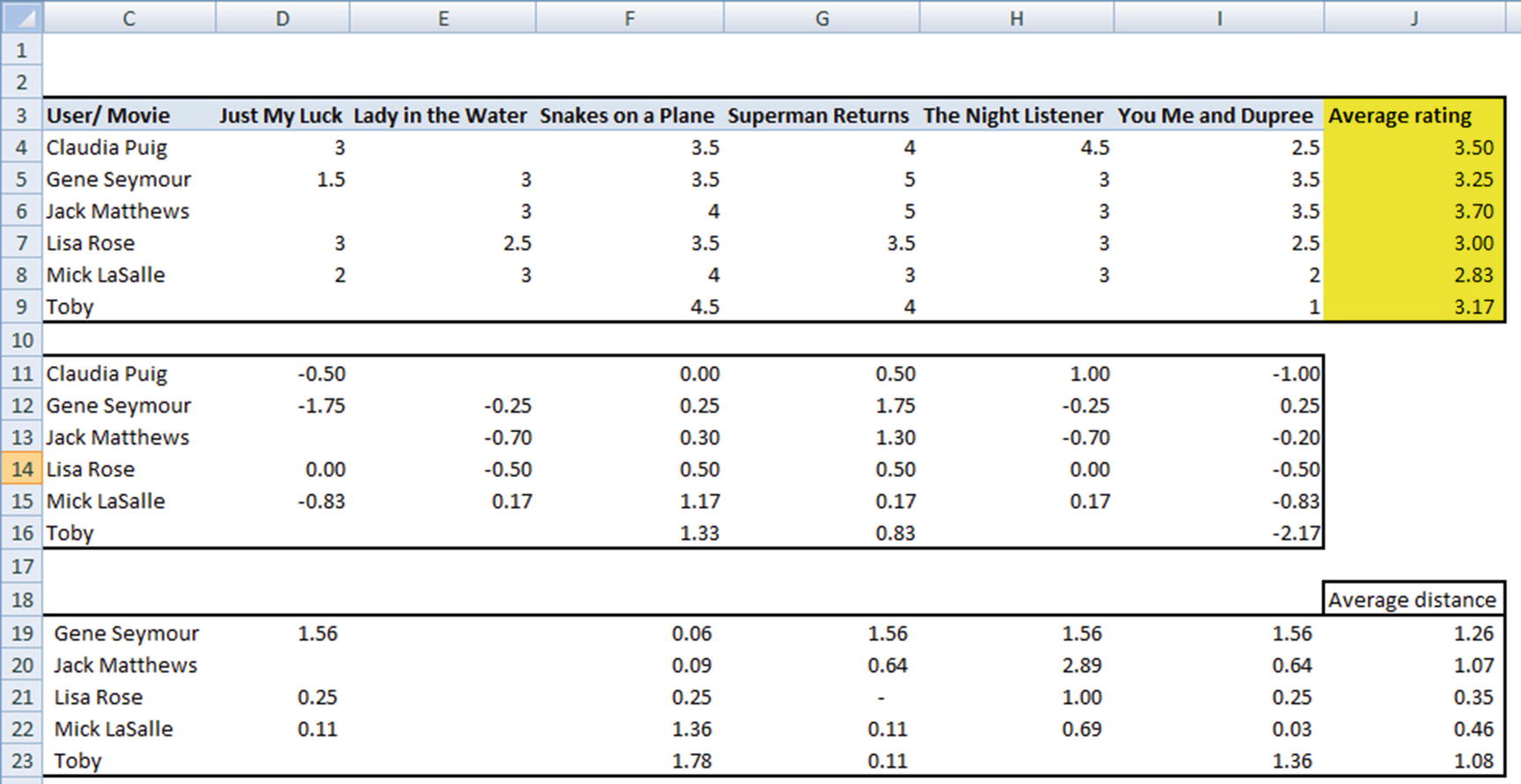
We can see that Lisa Rose is still the least distant (or closest, or most similar) user to Claudia Puig. Lisa rated Lady in the Water 0.50 units lower than her average movie rating of 3.00, which works out to ~8% lower than her average rating. Given that Lisa is the most similar user to Claudia, we would expect Claudia’s rating to likewise be 8% less than her average rating, which works out to the following:
3.5 × (1 – 0.5 / 3) = 2.91
Issue with Considering a Single User
So far, we have considered the single user who is most similar to Claudia. In practice, more is always better—that is, identifying the weighted average rating that k most similar users to a given user give is better than identifying the rating of the most similar user.
However, we need to note that not all k users are equally similar. Some are more similar, and others are less similar. In other words, some users’ ratings should be given more weightage, and other users’ ratings should be given less weightage. But using the distance-based metric, there is no easy way to come up with a similarity metric.
Cosine similarity as a metric comes in handy to solve this problem.
Cosine Similarity
Movie1 | Movie2 | Movie3 | |
|---|---|---|---|
User1 | 1 | 2 | 2 |
User2 | 2 | 4 | 4 |
In the preceding table, we see that both users’ ratings are highly correlated with each other. However, there is a difference in the magnitude of ratings.
If we were to compute Euclidian distance between the two users, we would notice that the two users are very different from each other. But we can see that the two users are similar in the direction (trend) of their ratings, though not in the magnitude of their ratings. The problem where the trend of users is similar but not the magnitude can be solved using cosine similarity between the users.

A and B are the vectors corresponding to user 1 and user 2 respectively.
Numerator of the given formula = (1 × 2 + 2 × 4 + 2 × 4) = 18
- Denominator of the given formula =×


Similarity = 18 / 18 = 1.
Based on the given formula, we can see that, on the basis of cosine similarity, we are in a position to assign high similarity to users that are directionally correlated but not necessarily in magnitude.
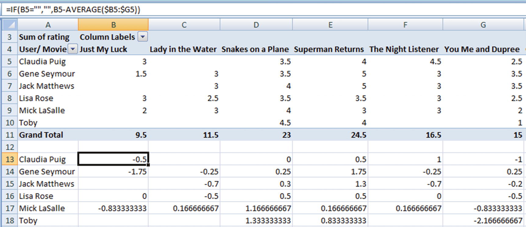
- 1.
Normalize users.
- 2.
Calculate the cosine similarity of rest of the users for a given user.
- 1.Normalize user ratings:
- 2.Calculate the numerator part of the cosine similarity calculation:
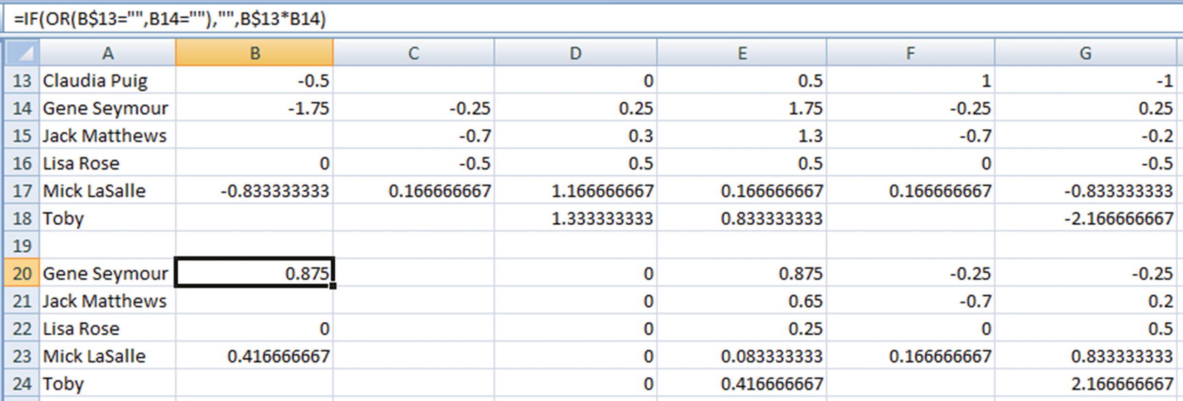 The numerator would be as follows:
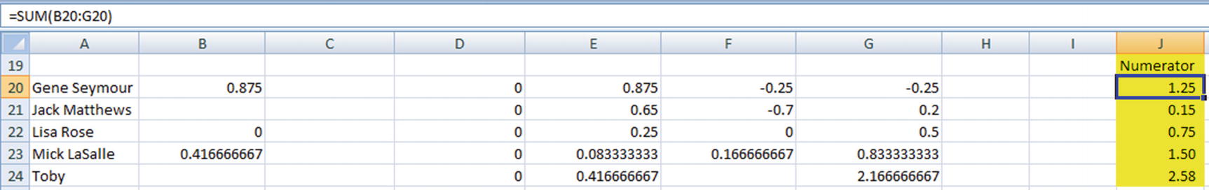
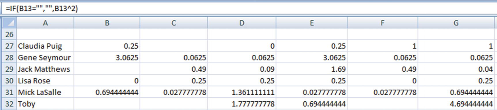
- 3.Prepare the denominator calculator of cosine similarity:
- 4.Calculate the final cosine similarity, as follows:
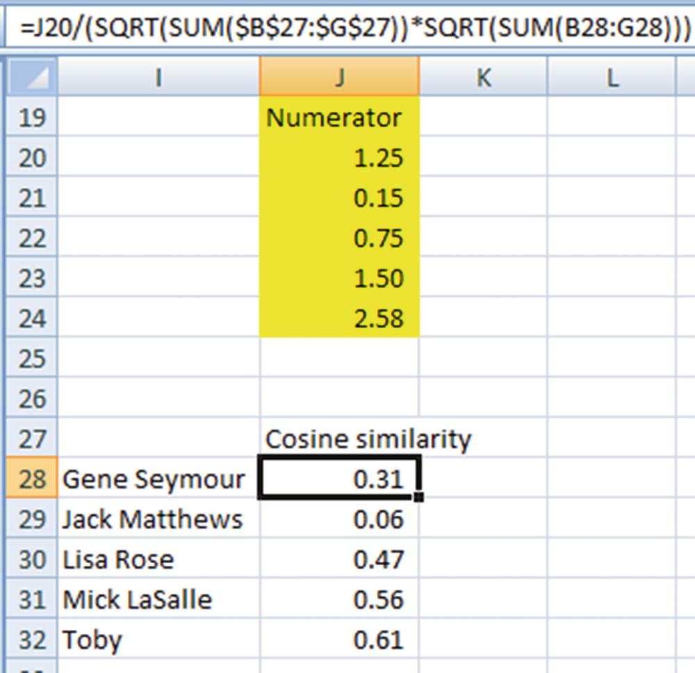
We now have a similarity value that is associated between –1 and +1 that gives a score of similarity for a given user.
We have now overcome the issue we faced when we had to consider the ratings given by multiple users in predicting the rating that a given user is likely to give to a movie. Users who are more similar to a given user can now be calculated.
- 1.
Normalize users.
- 2.
Calculate cosine similarity.
- 3.
Calculate the weighted average normalized rating.
- 1.
Identify the two most similar users who have also given a rating to the movie Lady in the Water.
- 2.
Calculate the weighted average normalized rating that they gave to the movie.
In this case, Lisa and Mick are the two most similar users to Claudia who have rate Lady in the Water. (Note that even though Toby is the most similar user, he has not rated Lady in the Water and so we cannot consider him for rating prediction.)
Weighted Average Rating Calculation
Similarity | Normalized rating | |
|---|---|---|
Lisa Rose | 0.47 | –0.5 |
Mick LaSalle | 0.56 | 0.17 |
The weighted average rating would now be as follows:
(0.47 × –0.5 + 0.56 × 0.17) / (0.47 + 0.56) = –0.14
Potentially, Claudia’s average rating would now be reduced by 0.14 to come up with the predicted rating of Claudia for the movie Lady in the Water.
Similarity | Normalized rating | Average rating | % avg rating | |
|---|---|---|---|---|
Lisa Rose | 0.47 | –0.5 | 3 | –0.5 / 3 = –0.16 |
Mick LaSalle | 0.56 | 0.17 | 2.83 | 0.17 / 2.83 = 0.06 |
Weighted average normalized rating percentage would now be as follows:
(0.47 × –0.16 + 0.56 × 0.06) / (0.47 + 0.56) = –0.04
Thus, the average rating of Claudia can potentially be reduced by 4% to come up with the predicted rating for the movie Lady in the Water.
Choosing the Right Approach
In recommender systems, there is no fixed technique that is proven to always work. This calls for a typical train, validate, and test scenario to come up with the optimal parameter combination .
Optimal number of similar users to be considered
Optimal number of common movies rated together by users before a user is eligible to be considered for similar user calculation
Weighted average rating calculation approach (based on percentage or on absolute value)
We can iterate through multiple scenarios of various combinations of the parameters, calculate the test dataset accuracy, and decide that the combination that gives the least error rate is the optimal combination for the given dataset.
Calculating the Error
Mean squared error (MSE) of all predictions made on the test dataset
Number of recommended items that a user bought in the next purchase
Note that although MSE helps in building the algorithm, in practice we might be measuring our model’s performance as a business-related outcome, as in the second case.
Issues with UBCF
One of the issues with user-based collaborative filtering is that every user has to be compared with every other user to identify the most similar user. Assuming there are 100 customers, this translates into the first user being compared to 99 users, the second user being compared to 98 users, the third to 97, and so on. The total comparisons here would be as follows:
99 + 98 + 97 + … + 1 + 0 = 99 × (99 + 1) / 2 = 4950
For a million customers, the total number of comparisons would look like this:
999,999 × 1,000,000 / 2 = ~500,000,000,000
That’s around 500 billion comparisons. The calculations show that the number of comparisons to identify the most similar customer increases exponentially as the number of customers increases. In production, this becomes a problem because if every user’s similarity with every other user needs to be calculated every day (since user preferences and ratings get updated every day based on the latest user data), one would need to perform ~500 billion comparisons every day.
To address this problem, we can consider item-based collaborative filtering instead of user-based collaborative filtering.
Item-Based Collaborative Filtering
Given that the number of computations is an issue in UBCF, we will modify the problem so that we observe the similarity between items and not users. The idea behind item-based collaborative filtering (IBCF) is that two items are similar if the ratings that they get from the same users are similar. Given that IBCF is based on items and not on user similarity, it doesn’t have the problem of performing billions of computations.
Let’s assume that there are a total of 10,000 movies in a database and 1 million customers attracted to the site. In this case, if we perform UBCF, we would be performing ~500 billion similarity calculations. But using IBCF, we would be performing 9,999 × 5,000 = ~ 50 million similarity calculations.
We can see that the number of similarity calculations increases exponentially as the number of customers grows. However, given that the number of items (movie titles, in our case) is not expected to experience the same growth rate as the number of customers, in general IBCF is less computationally sensitive than UBCF.
The way in which IBCF is calculated and the techniques involved are very similar to UBCF. The only difference is that we would work on a transposed form of the original movie matrix we saw in the previous section. This way, the rows are not of users, but of movies.
Note that although IBCF is better than UBCF in terms of computation, the number of computations is still very high.
Implementing Collaborative Filtering in R
In this code, we have reshaped our data so that it can be converted into a realRatingMatrix class that gets consumed by the Recommender function to provide the missing value predictions.
Implementing Collaborative Filtering in Python
- 1.
Import the dataset:
import pandas as pdimport numpy as npt=pd.read_csv("D:/book/Recommender systems/movie_rating.csv") - 2.
Convert the dataset into a pivot table:
t2 = pd.pivot_table(t,values='rating',index='critic',columns='title') - 3.
Reset the index:
t3 = t2.reset_index()t3=t3.drop(['critic'],axis=1) - 4.
Normalize the dataset:
t4=t3.subtract(np.mean(t3,axis=1),axis=0) - 5.
Drop the rows that have a missing value for Lady in the Water:
t5=t4.loc[t4['Lady in the Water'].dropna(axis=0).index]t6=t5.reset_index()t7=t6.drop(['index'],axis=1) - 6.
Calculate the distance of every other user to Claudia:
x=[]for i in range(t7.shape[0]):x.append(np.mean(np.square(t4.loc[0]-t7.loc[i])))t6.loc[np.argmin(x)]['Lady in the Water'] - 7.
Calculate the predicted rating of Claudia :
np.mean(t3.loc[0]) * (1+(t6.loc[np.argmin(x)]['Lady in the Water']/np.mean(t3.loc[3])))
Working Details of Matrix Factorization
Although user-based or item-based collaborative filtering methods are simple and intuitive, matrix factorization techniques are usually more effective because they allow us to discover latent features underlying the interactions between users and items.
In matrix factorization, if there are U users, each user is represented in K columns, thus we have a U × K user matrix. Similarly, if there are D items, each item is also represented in K columns, giving us a D × K matrix.
A matrix multiplication of the user matrix and the transpose of the item matrix would result in the U × D matrix, where U users may have rated on some of the D items.
The K columns could essentially translate into K features, where a higher or lower magnitude in one or the other feature could give us an indication of the type or genre of the item. This gives us the ability to know the features that a user would give a higher weightage to or the features that a user might not like. Essentially, matrix factorization is a way to represent users and items in such a way that the probability of a user liking or purchasing an item is high if the features that correspond to an item are the features that the user gives a higher weightage to.
User | Movies | Actual |
|---|---|---|
1 | 1 | 5 |
1 | 2 | 3 |
1 | 3 | |
1 | 4 | 1 |
2 | 1 | 4 |
2 | 2 | |
2 | 3 | |
2 | 4 | 1 |
3 | 1 | 1 |
3 | 2 | 1 |
3 | 3 | |
3 | 4 | 5 |
4 | 1 | 1 |
4 | 2 | |
4 | 3 | |
4 | 4 | 4 |
5 | 1 | |
5 | 2 | 1 |
5 | 3 | 5 |
5 | 4 | 4 |
Our task is to predict the missing values in the Actual column, which indicate that the user has not rated the movie yet.
- 1.
Initialize the values of P matrix randomly, where P is a U × K matrix. We’ll assume a value of k = 2 for this example.
A better way of randomly initializing the values is by limiting the values to be between 0 and 1.
In this scenario, the matrix of P will be a 5 × 2 matrix, because k = 2 and there are 5 users: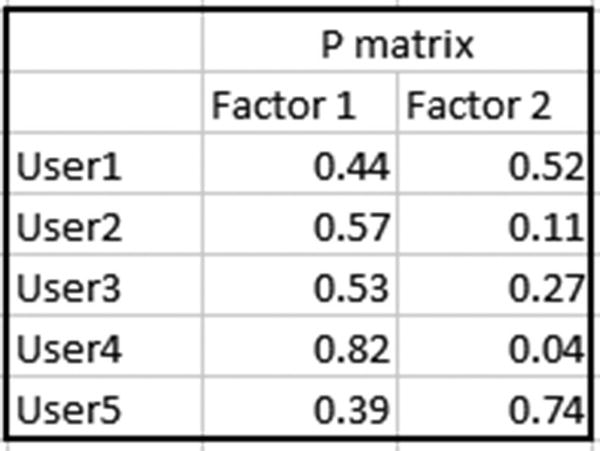
- 2.
Initialize the values of Q matrix randomly, again where Q is a K × D matrix—that is, a 2 × 4 matrix, because there are four movies, as shown in the first table.
The Q matrix would be as follows: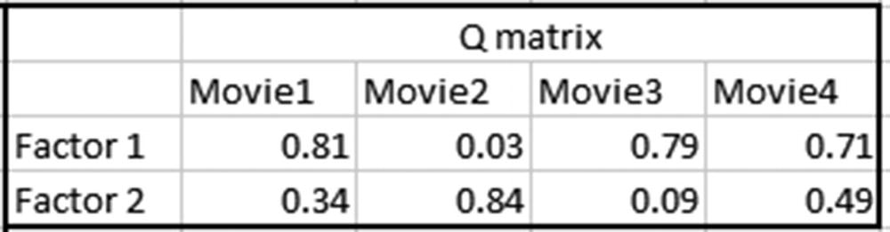
- 3.
Calculate the value of the matrix multiplication of P × Q matrix.
Note that the Prediction column in the following is calculated by the matrix multiplication of P matrix and Q matrix (I will discuss the Constraint column in the next step):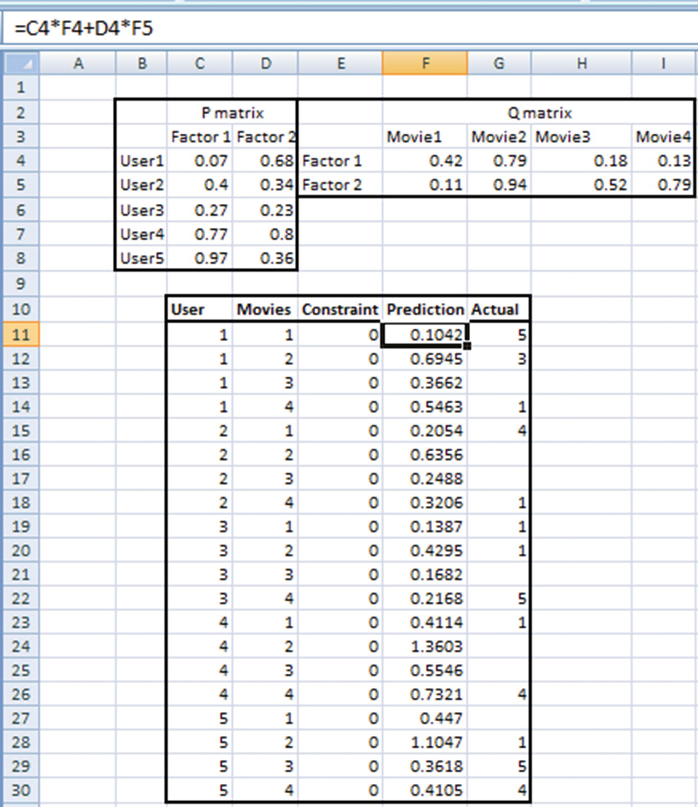
- 4.
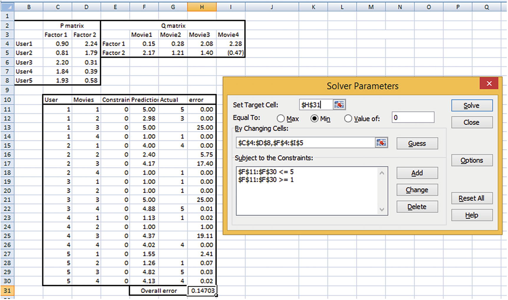
Specify the optimization constraints.
The predicted value (the multiplication of each element of the two matrices) should ideally be equal to the ratings of the big matrix. The error calculation is based on the typical squared error calculation and is done as follows (note that the weight values in P and matrices have varied because they are random numbers and are initialized using the randbetween function, which changes values every time Enter is pressed in Excel):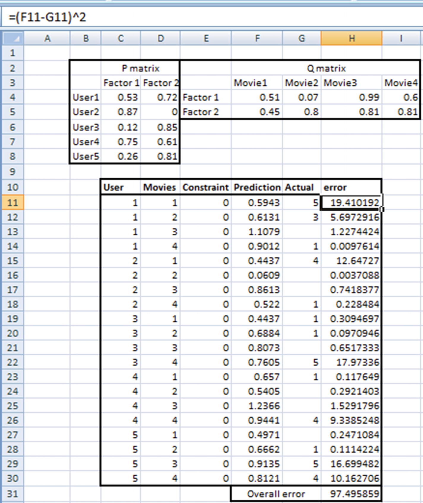
Objective : Change the randomly initialized values of P and Q matrices to minimize overall error.
Constraint : No prediction can be greater than 5 or less than 1.
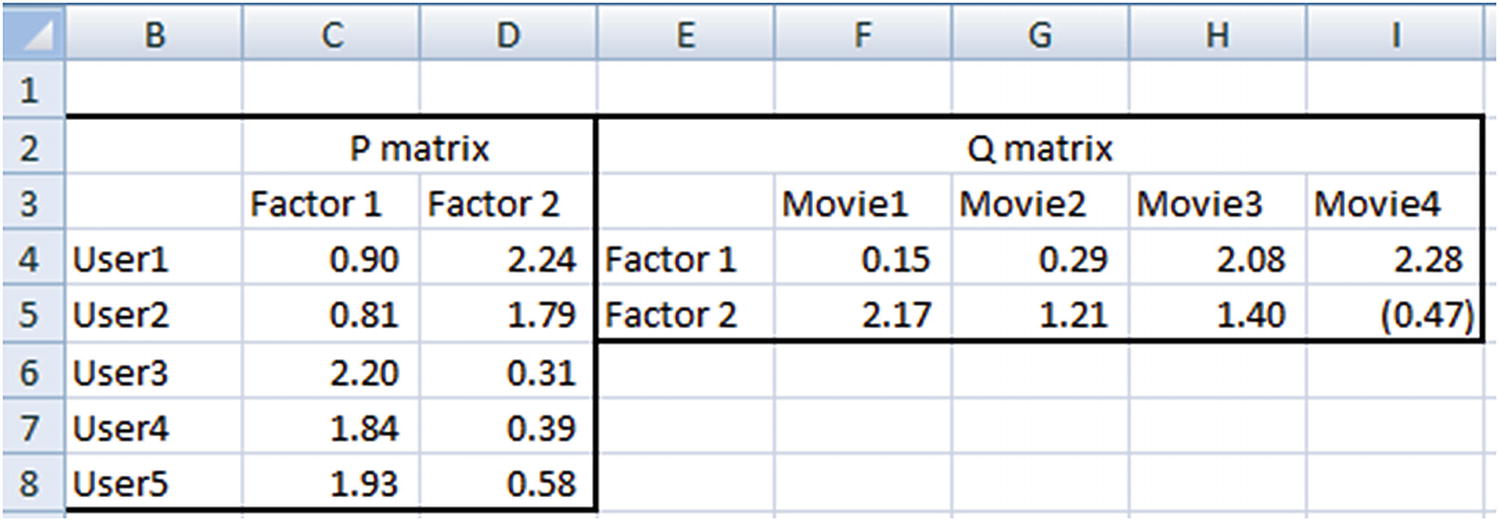
Insights on P AND Q MATRICES
In P matrix, user 1 and user 2 have similar weightages for factors 1 and 2, so they can potentially be considered to be similar users.
Also, the way in which user 1 and 2 have rated movies is very similar—the movies that user 1 rated highly have a high rating from user 2 as well. Similarly, the movies that user 1 rated poorly also had low ratings from user 2.
The same goes for the interpretation for Q matrix (the movie matrix). Movie 1 and movie 4 have quite some distance between them. We can also see that, for a majority of users, if the rating given for movie 1 is high, then movie 4 got a low rating, and vice versa.
Implementing Matrix Factorization in Python
Notice that the P matrix and Q matrix are obtained through Excel’s Solver, which essentially runs gradient descent in the back end. In other words, we are deriving the weights in a manner similar to the neural networks–based approach, where we are trying to minimize the overall squared error.
User | Movies | Actual |
|---|---|---|
1 | 4 | 1 |
2 | 4 | 1 |
3 | 1 | 1 |
3 | 2 | 1 |
4 | 1 | 1 |
5 | 2 | 1 |
1 | 2 | 3 |
2 | 1 | 4 |
4 | 4 | 4 |
5 | 4 | 4 |
1 | 1 | 5 |
3 | 4 | 5 |
5 | 3 | 5 |
The function Embedding helps in creating vectors similar to the way we converted a word into a lower-dimensional vector in Chapter 8.
Implementing Matrix Factorization in R
Although matrix factorization can be implemented using the kerasR package, we will use the recommenderlab package (the same one we worked with for collaborative filtering).
- 1.
Import the relevant packages and dataset:
# Matrix factorizationt=read.csv("D:/book/Recommender systems/movie_rating.csv")library(reshape2)library(recommenderlab) - 2.
Pre-process the data:
t2=acast(t,critic~title)t2# Convert it as a matrixR<-as.matrix(t2)# Convert R into realRatingMatrix data structure# RealRatingMatrix is a recommenderlab sparse-matrix like data-structurer <- as(R, "realRatingMatrix") - 3.
Use the funkSVD function to build the matrix factors:
fsvd <- funkSVD(r, k=2,verbose = TRUE)p <- predict(fsvd, r, verbose = TRUE)pNote that the object p constitutes the predicted ratings of all the movies across all the users.
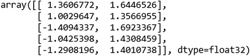
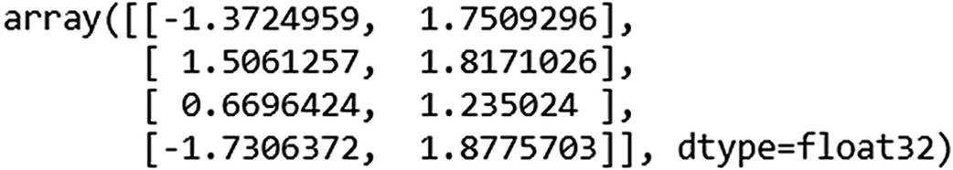
The object fsvd constitutes the user and item matrices , and they can be obtained with the following code:
str(fsvd)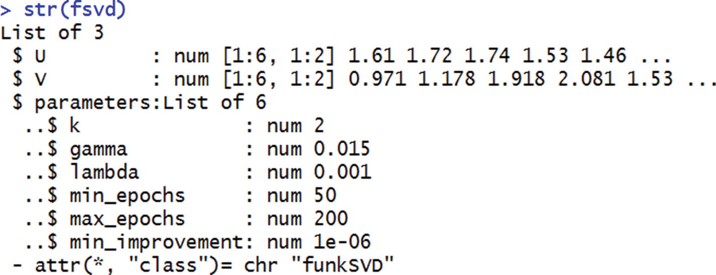
The user matrix can thus be accessed as fsvd$U, and the item matrix by fsvd$V. The parameters are the learning rate and the epochs parameters we learned about in Chapter 7.
Summary
The major techniques used to provide recommendations are collaborative filtering and matrix factorization.
Collaborative filtering is extremely prohibitive in terms of the large number of computations.
Matrix factorization is less computationally intensive and in general provides better results.
Ways to build matrix factorization and collaborative filtering algorithms in Excel, Python, and R