The dictionary meaning of clustering is grouping. In data science, too, clustering is an unsupervised learning technique that helps in grouping our data points.
For a business user to understand the various types of users among customers
To make business decisions at a cluster (group) level rather than at an overall level
To help improve the accuracy of predictions, since different groups exhibit different behavior, and hence a separate model can be made for each group
Different types of clustering
How different types of clustering work
Use cases of clustering
Intuition of clustering
Scenario 1: A store manager is evaluated solely on the sales made. We’ll rank order all the store managers by the sales their stores have made, and the top-selling store managers receive the highest reward.
Drawback: The major drawback of this approach is that we are not taking into account that some stores are in cities, which typically have very high sales when compared to rural stores. The biggest reason for high sales in city stores could be that the population is high and/or the spending power of city-based customers is higher.
Scenario 2: If we could divide the stores into city and rural, or stores that are frequented by customers with high purchasing power, or stores that are frequented by populations of a certain demographic (say, young families) and call each of them a cluster, then only those store managers who belong to the same cluster can be compared.
For example, if we divide all the stores into city stores and rural stores, then all the store managers of city stores can be compared with each other, and the same would be the case with rural store managers.
Drawback: Although we are in a better place to compare the performance of different store managers, the store managers can still be compared unfairly. For example, two city stores could be different—one store is in the central business district frequented by office workers, and another is in a residential area of a city. It is quite likely that central business district stores inherently have higher sales among the city stores.
Although scenario 2 still has a drawback, it is not as bad a problem as in scenario 1. Thus clustering into two kinds of stores helps a little as a more accurate way of measuring store manager performance.
Building Store Clusters for Performance Comparison
In scenario 2, we saw that the store managers can still question the process of comparison as unfair—because stores can still differ in one or more parameters.
Differences in products that are sold in different stores
Differences in the age group of customers who visit the store
Differences in lifestyles of the customers who visit the store
City store versus rural store
High-products store versus low-products store
High-age-group-customers store versus low-age-group-customers store
Premium-shoppers store versus budget-shoppers store
We can create a total of 16 different clusters (groups) based on just the factors listed (the exhaustive list of all combinations results in 16 groups).
We talked about the four important factors that differentiate the stores, but there could still be many other factors that differentiate among stores. For example, a store that is located in a rainier part of the state versus a store that is located in a sunnier part.
In essence, stores differ from each other in multiple dimensions/factors. But results of store managers might differ significantly because of certain factors, while the impact of other factors could be minimal.
Ideal Clustering
So far, we see that each store is unique, and there could be a scenario where a store manager can always cite one reason or another why they cannot be compared with other stores that fall into the same cluster. For example, a store manager can say that although all the stores that belong to this group are city stores with majority of premium customers in the middle-aged category, their store did not perform as well as other stores because it is located close to a competitor store that has been promoting heavily—hence, the store sales were not that high when compared to other stores in the same group.
Thus, if we take all the reasons into consideration, we might end up with a granular segmentation to the extent that there is only store in each cluster. That would result in a great clustering output, where each store is different, but the outcome would be useless because now we cannot compare across stores.
Striking a Balance Between No Clustering and Too Much Clustering: K-means Clustering
We’ve seen that having as many clusters as there are stores is a great cluster that differentiates among each store, but it’s a useless cluster since we cannot draw any meaningful results from it. At the same time, having no cluster is also bad because store managers might be compared inaccurately with store mangers of completely different stores.
Thus, using the clustering process, we strive towards striking a balance. We want to identify the few factors that differentiate the stores as much as possible and consider only those for evaluation while leaving out the rest. The means of identifying the few factors that differentiate among the stores as much as possible is achieved using k-means clustering.
To see how k-means clustering works, let’s consider a scenario: you are the owner of a pizza chain. You have a budget to open three new outlets in a neighborhood. How do you come up with the optimal places to open the three outlets?
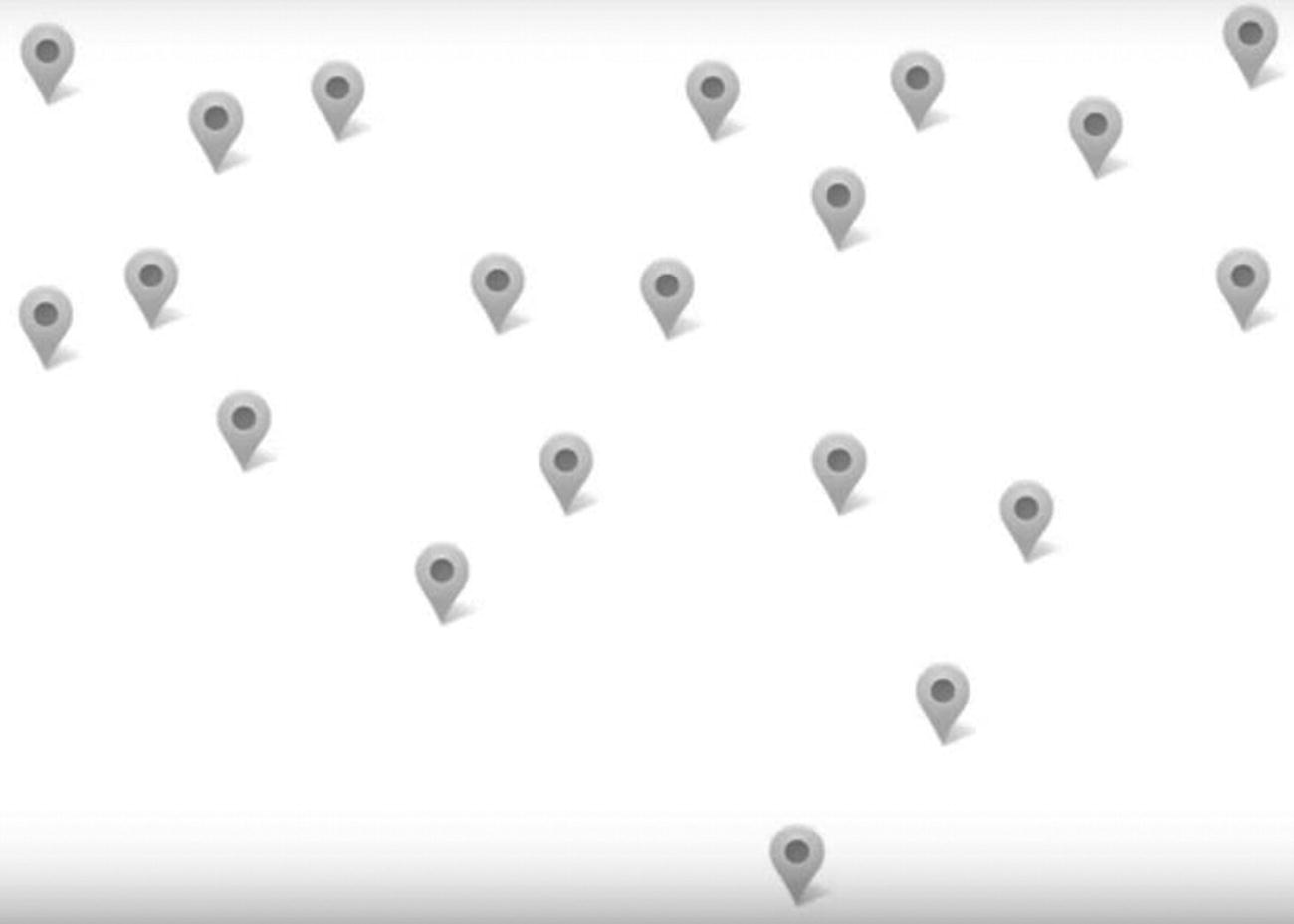
Each marker represents a household
The circles represent potential outlet locations
- 1.
Minimize the distance of each household to the nearest pizza outlet
- 2.
Maximize the distance between each pizza outlet
Assume for a second that a pizza outlet can deliver to two houses only. If the demand from both houses is uniform, would it be better to locate the pizza outlet exactly between the houses or closer to one or the other house? If it takes 15 minutes to deliver to house A and 45 minutes to deliver to house B, intuitively we would seem to be better off locating the outlet where the time to deliver to either house is 30 minutes—that is, at a point exactly between the two houses. If that were not the case, the outlet might often fail on its promise to deliver within 45 minutes for house B, while never failing to keep its promises to household A.
The Process of Clustering
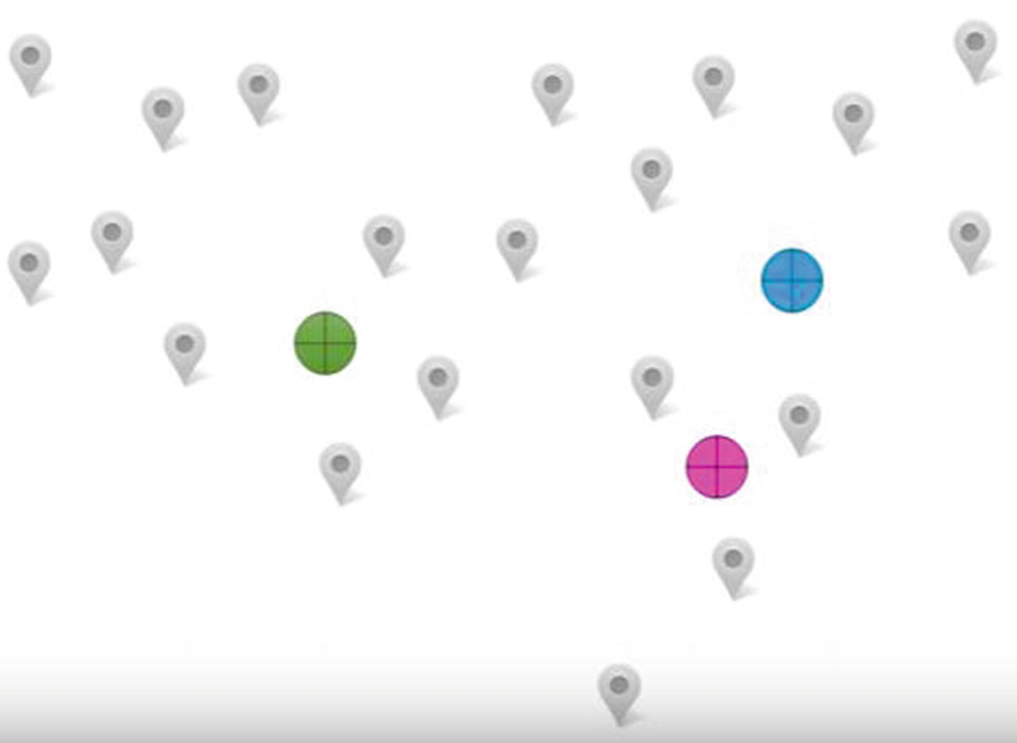
- 1.Randomly come up with three places where we can start outlets, as shown in Figure 11-3.
 Figure 11-3
Random locations
- 2.Measure the distance of each house to the three outlet locations. The outlet that is closest to the household delivers to the household. The scenario would look like Figure 11-4.
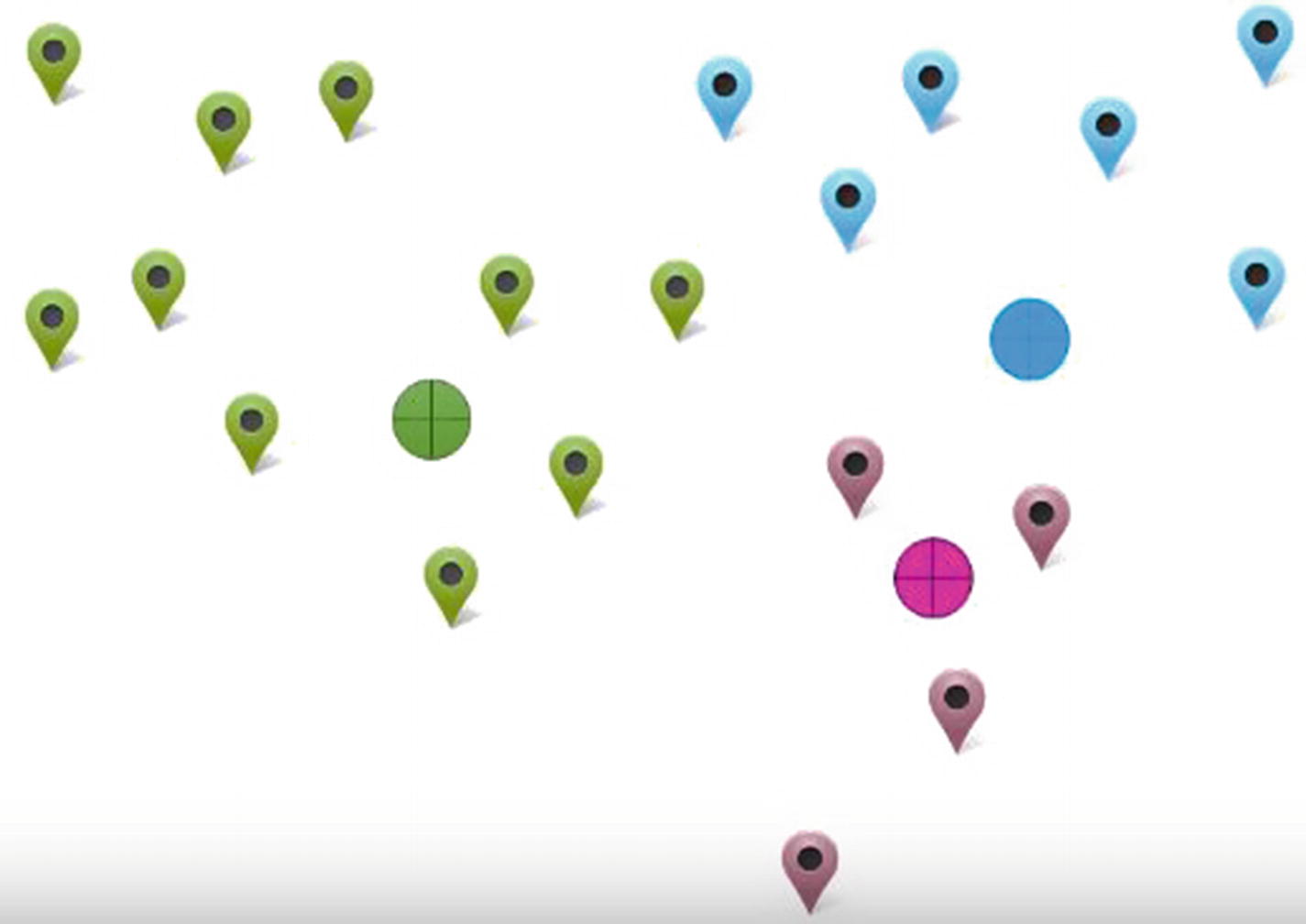 Figure 11-4
Better informed locations
- 3.As we saw earlier, we are better off if the delivery outlet is in the middle of households than far away from the majority of the households. Thus, let’s change our earlier planned outlet location to be in the middle of the households (Figure 11-5).
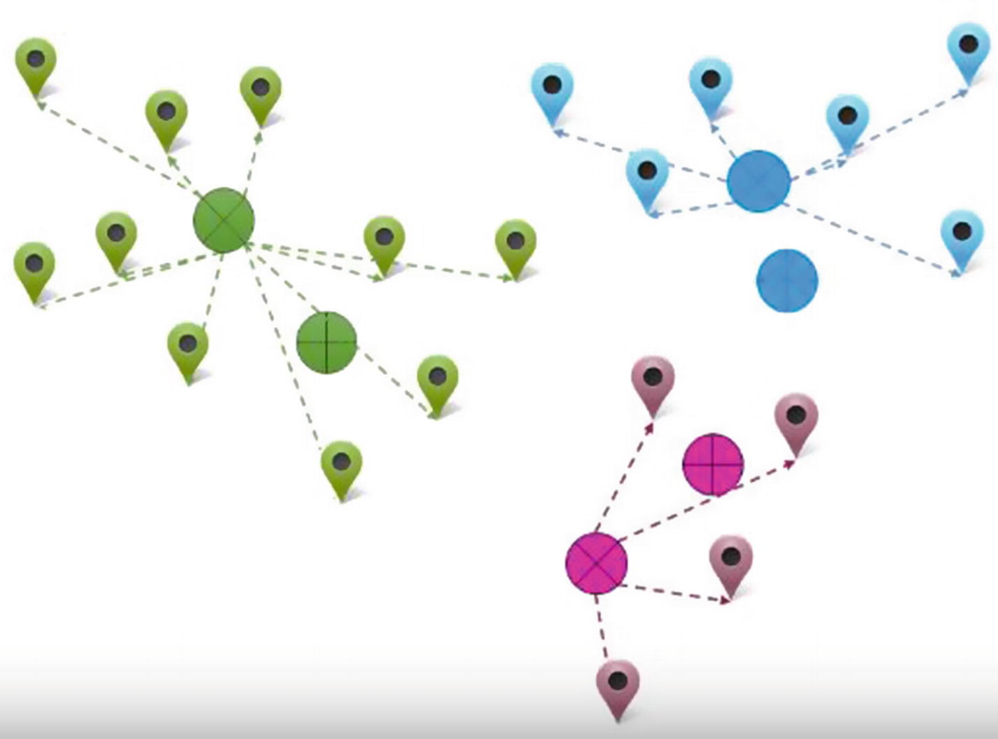 Figure 11-5
Locations in the middle
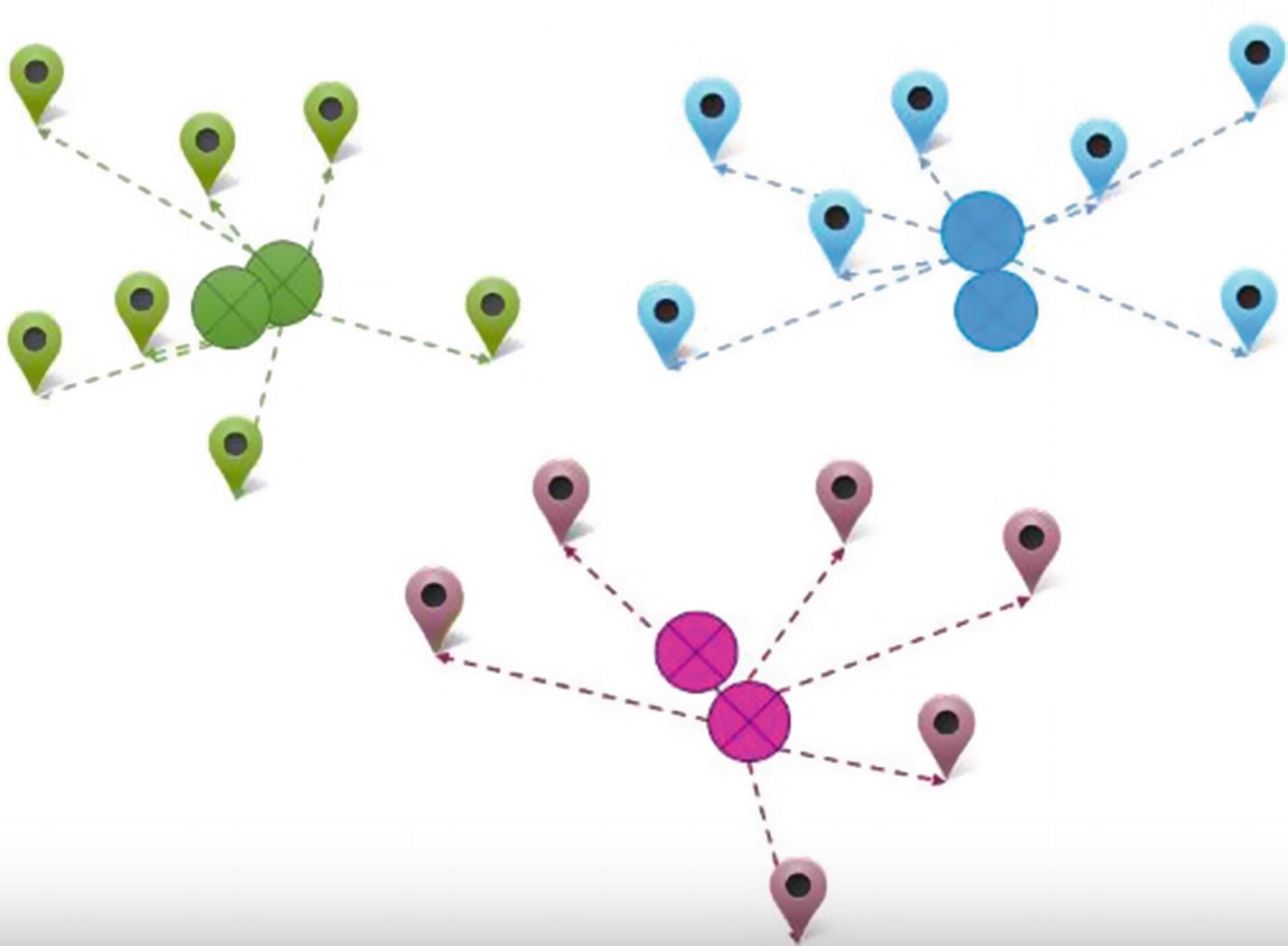
- 4.We see that the delivery outlet locations have changed to be more in the middle of each group. But because of the change in location, there might be some households that are now closer to a different outlet. Let’s reassign households to stores based on their distance to different stores (Figure 11-6).
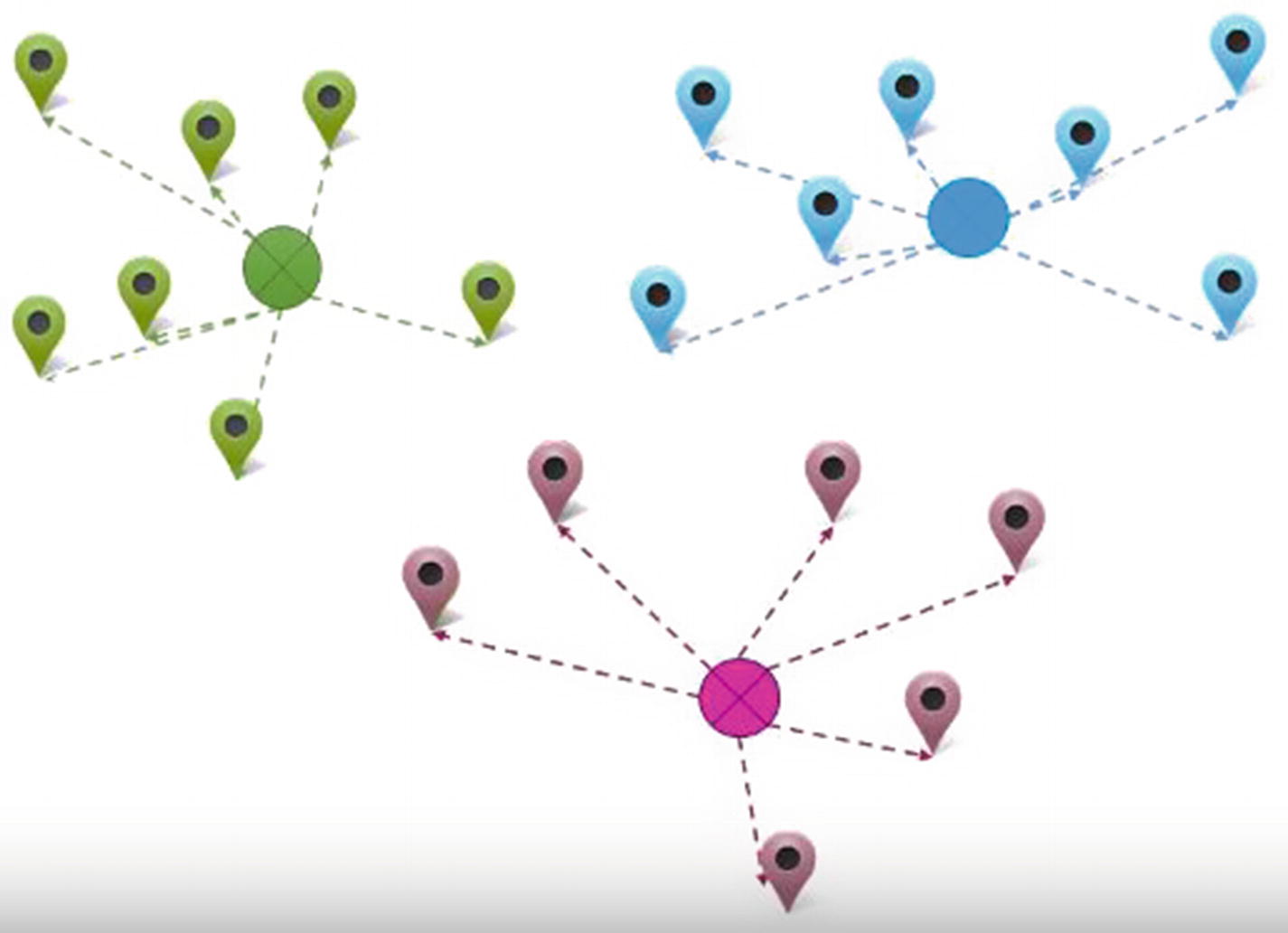 Figure 11-6
Reassigning households
- 5.
- 6.
Now that the cluster centers have changed, there is now another a chance that the households need to be reassigned to a different outlet than the current one.
The steps continue until there is no further reassignment of households to different clusters, or a maximum of a certain number of iterations is reached.
As you can see, we can in fact come up a more scientific/analytical way of finding optimal locations where the outlets can be opened.
Working Details of K-means Clustering Algorithm
We will be opening three outlets, so we came up with three groups of households, where each group is served by a different outlet.
The k in k-means clustering stands for the number of groups we will be creating in the dataset we have. In some of the steps in the algorithm we went through in the preceding section, we kept updating the centers once some households changed their group from one to another. The way we were updating centers is by taking the mean of all the data points, hence k-means.
Finally, after going through the steps as described, we ended up with three groups of three datapoints or three clusters from the original dataset.
Applying the K-means Algorithm on a Dataset
X | Y | Cluster |
|---|---|---|
5 | 0 | 1 |
5 | 2 | 2 |
3 | 1 | 1 |
0 | 4 | 2 |
2 | 1 | 1 |
4 | 2 | 2 |
2 | 2 | 1 |
2 | 3 | 2 |
1 | 3 | 1 |
5 | 4 | 2 |
Let X and Y be the independent variables that we want our clusters to be based on. Let’s say we want to divide this dataset into two clusters.
In the first step, we initialize the clusters randomly. So, the cluster column in the preceding table is randomly initialized.
Centroid | 1 | 2 |
|---|---|---|
X | 2.6 | 3.2 |
Y | 1.4 | 3 |
Note that the value 2.6 is the average of all the values of X that belong to cluster 1. Similarly, the other centers are calculated.
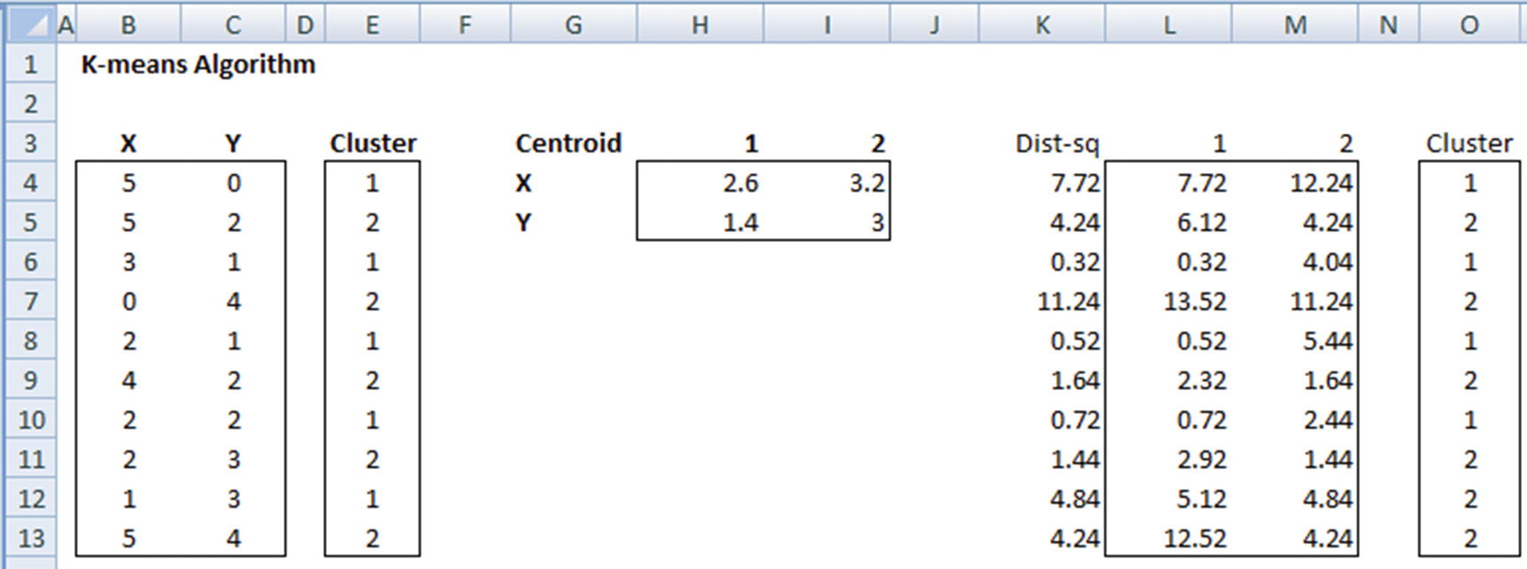
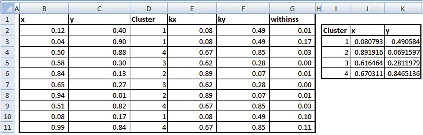
In columns L & M we have calculated the distance of each point to the two cluster centers. The cluster center in column O is updated by looking at the cluster that has minimum distance with the data point.
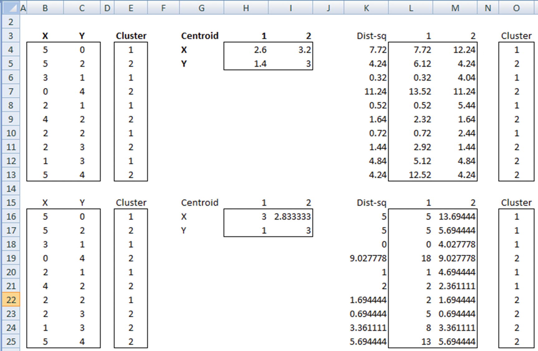
We keep on iterating the process until there is no further change in the clusters that data points belong to. If a data point cluster keeps on changing, we would potentially stop after a few iterations.
Properties of the K-means Clustering Algorithm
- 1.
All points belonging to the same group are as close to each other as possible
- 2.
Each group’s center is as far away from other group’s center as possible
There are measures that help in assessing the quality of a clustering output based on these objectives.
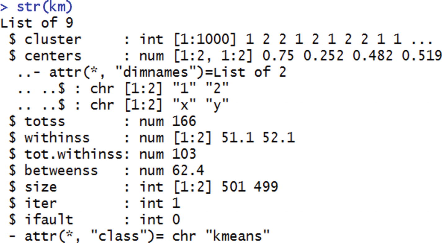
Totss (Total Sum of Squares)
In a scenario where the original dataset itself is considered as a cluster, the midpoint of the original dataset is considered as the center. Totss is the sum of the squared distance of all points to the dataset center.
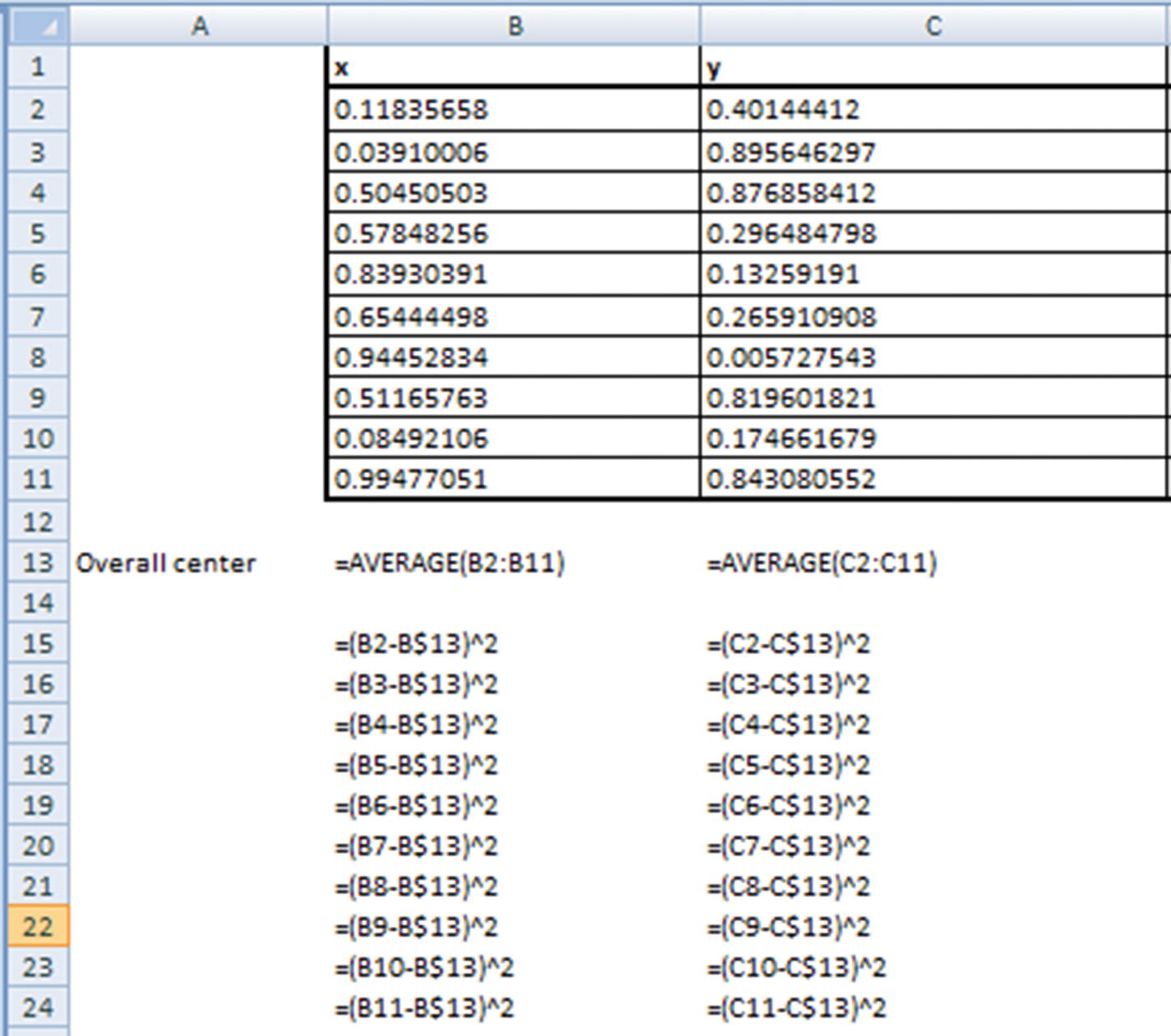
Total sum of squares would be the sum of all the values from cell B15 to cell C24.
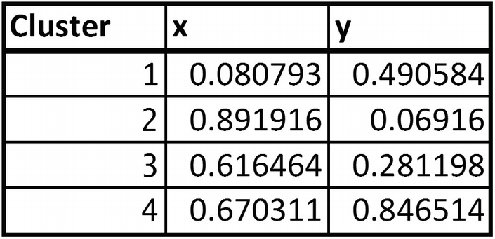
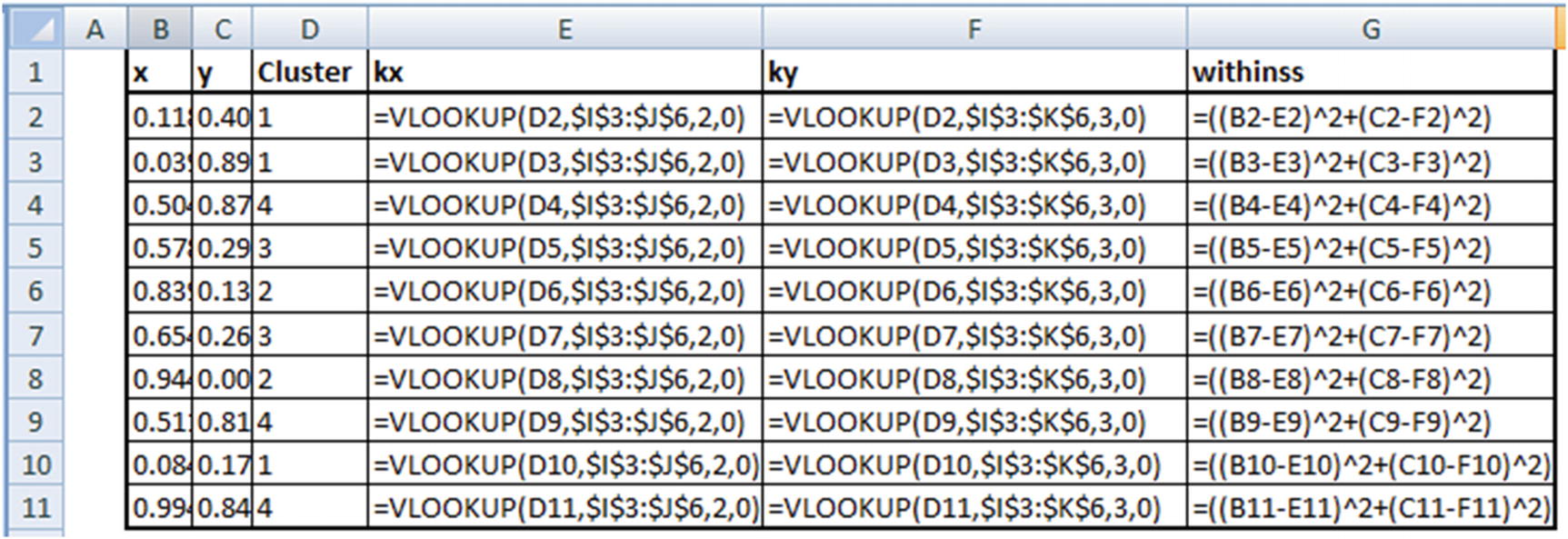
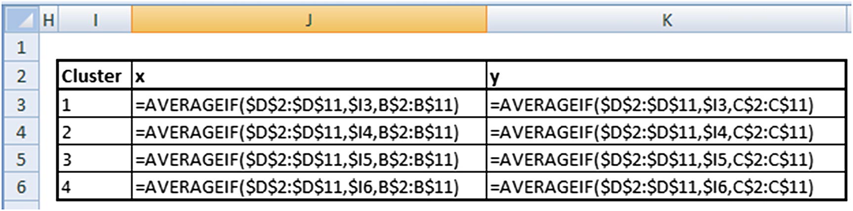
Cluster Centers
The cluster center of each cluster will be the midpoint (mean) of all the points that fall in the same cluster. For example, in the Excel sheet cluster centers are calculated in columns I and J. Note that this is just the average of all points that fall in the same cluster.
Tot.withinss
Tot.withinss is the sum of the squared distance of all points to their corresponding cluster center .
Betweenss
Betweenss is the difference between totss and tot.withinss.
Implementing K-means Clustering in R
Implementing K-means Clustering in Python
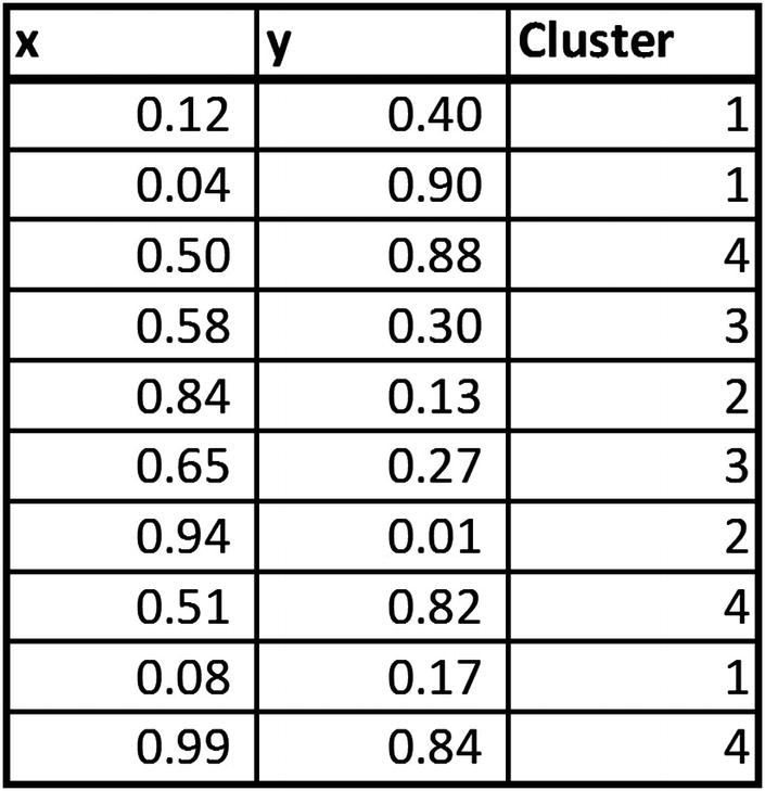
In that code snippet, we are extracting two clusters from the original dataset named data2. The resulting labels for each data point of which cluster they belong to can be extracted by specifying kmeans.labels_.
Significance of the Major Metrics
As discussed earlier, the objective of the exercise of clustering is to get all the data points that are very close to each other into one group and have groups that are as far away from each other as possible.
- 1.
Minimize intracluster distance
- 2.
Maximize intercluster distance
Let’s look at how the metrics discussed earlier help in achieving the objective. When there is no clustering (that is, all the dataset is considered as one cluster), the overall distance of each point to the cluster center (where there is one cluster) is totss. The moment we introduce clustering in the dataset, the sum of distance of each point within a cluster to the corresponding cluster centre is tot.withinss. Note that as the number of clusters increases, tot.withinss keeps on decreasing.
Consider a scenario where the number of clusters is equal to the number of data points. Tot.withinss is equal to 0 in that scenario, because the distance of each point to the cluster center (which is the point itself) is 0.
Thus, tot.withinss is a measure of intracluster distance. The lower the ratio of tot.withinss / totss, the higher quality is the clustering process.
However, we also need to note that the scenario where tot.withinss = 0 is the scenario where the clustering becomes useless, because each point is a cluster in itself.
In the next section, we’ll make use of the metric tot.withinss / totss in a slightly different way.
Identifying the Optimal K
One major question we have not answered yet is how to obtain the optimal k value? In other words, what is the optimal number of clusters within a dataset?
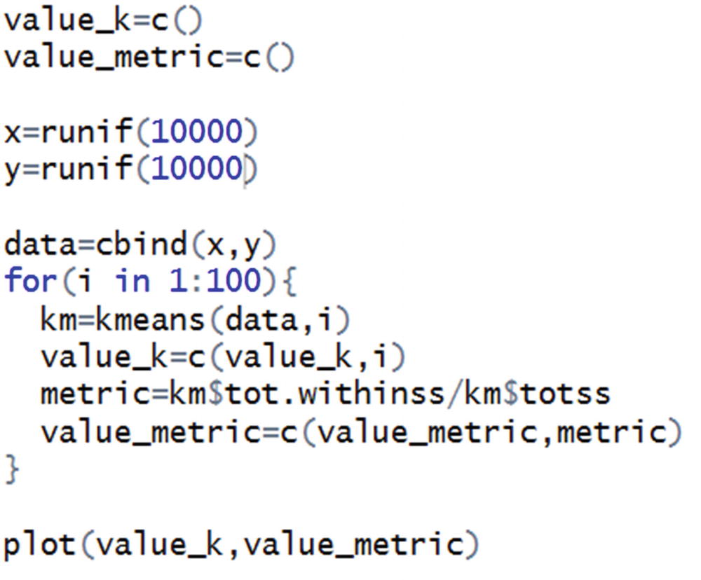
We are creating a dataset data with 10,000 randomly initialized x and y values.
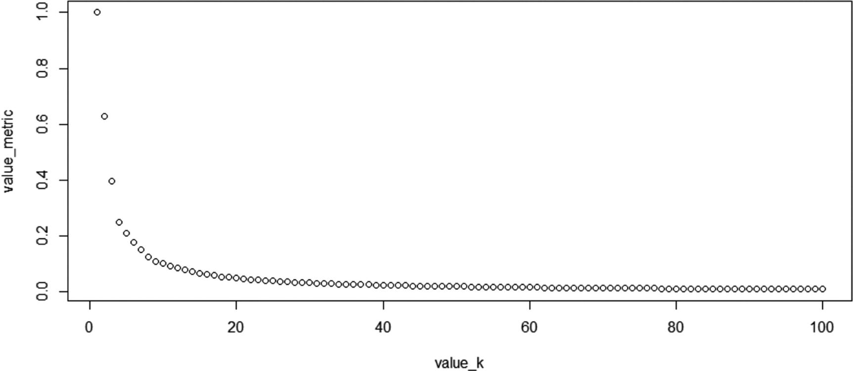
Variation in tot.withinss/totss over different values of k
Note that as the value of k is increased from k = 1 to k = 2, there is a steep decrease in the metric, and similarly, the metric decreased when k is reduced from 2 to 4.
However, as k is further reduced, the value of the metric does not decrease by a lot. So, it is prudent to keep the value of k close to 7 because maximum decrease is obtained up to that point, and any further decrease in the metric (tot.withinss / totss) does not correlate well with an increase in k.
Given that the curve looks like an elbow, it sometimes called the elbow curve .
Top-Down Vs. Bottom-Up Clustering
So far, in the process of k-means clustering, we don’t know the optimal number of clusters, so we keep trying various scenarios with multiple values of k. This is one of the relatively small problems with the bottom-up approach, where we start with an assumption that there is no cluster and slowly keep building multiple clusters, one at a time, till we find the optimal k based on the elbow curve.
Top-down clustering takes an alternative look at the same process. It assumes that each point is a cluster in itself and tries to combine points based on their distance from other points.
Hierarchical Clustering
Hierarchical clustering is a classic form of top-down clustering. In this process, the distance of each point to the rest of points is calculated. Once the distance is calculated, the points that are closest to the point in consideration are combined to form a cluster. This process is repeated across all points, and thus a final cluster is obtained.
The hierarchical part comes from the fact that we start with one point, combine it with another point, and then combine this combination of points with a third point, and keep on repeating this process.
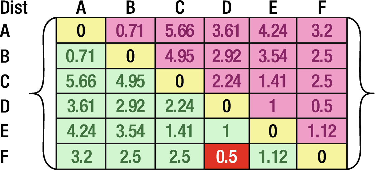
Distance of data points
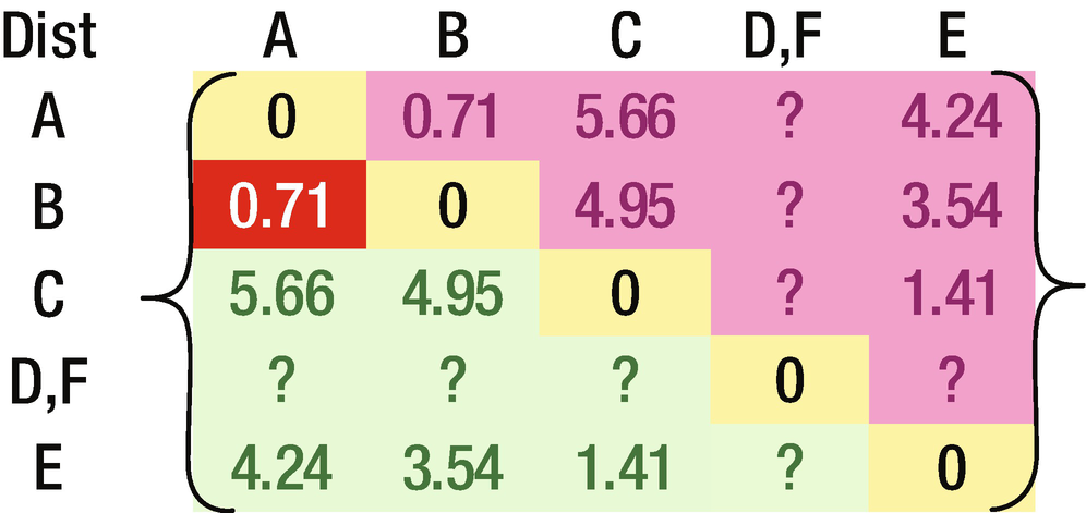
The resulting matrix

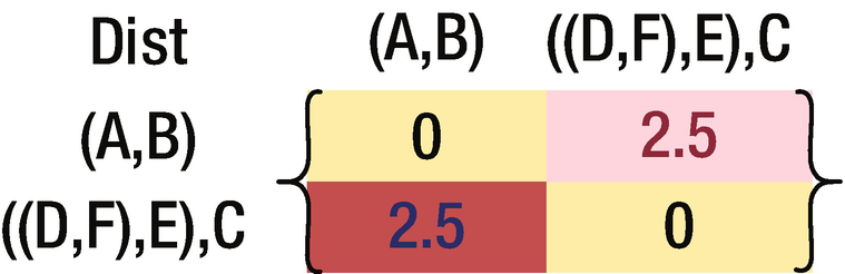
The final matrix
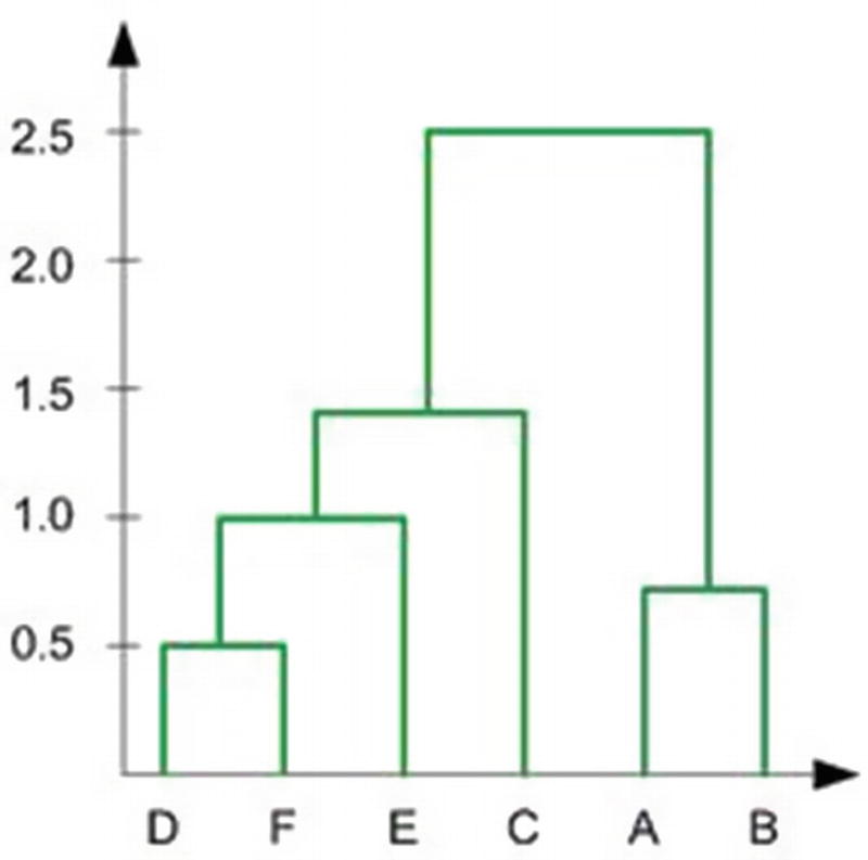
Representing the cluster
Major Drawback of Hierarchical Clustering
One of the major drawbacks of hierarchical clustering is the large number of calculations one needs to perform.
If there are 100 points in a dataset, say, then the first step is identifying the point that is closest to point 1 and so on for 99 computations. And for the second step, we need to compare the second point’s distance with the rest of the 98 points. This makes for a total of 99 × 100 / 2, or n × (n – 1) / 2 calculations when there are n data points, only to identify the combination of data points that have the least distance between them among all the combination of data points.
The overall computation becomes extremely complex as the number of data points increase from 100 to 1,000,000. Hence, hierarchical clustering is suited only for small datasets.
Industry Use-Case of K-means Clustering
We’ve calculated the optimal value of k using the elbow curve of the tot.withinss / totss metric. Let’s use a similar calculation for a typical application in building a model.
Let’s say we are fitting a model to predict whether a transaction is fraudulent or not using logistic regression. Given that we would be working on all the data points together, this translates into a clustering exercise where k = 1 on the overall dataset. And let’s say it has an accuracy of 90%. Now let’s fit the same logistic regression using k = 2, where we have a different model for each cluster. We’ll measure the accuracy of using two models on the test dataset.
We keep repeating the exercise by increasing the value of k—that is, by increasing the number of clusters. Optimal k is where we have k different models, one each for each cluster and also the ones that achieve the highest accuracy on top of the test dataset. Similarly, we would use clustering to understand the various segments that are present in the dataset.
Summary
K-means clustering helps in grouping data points that are more similar to each other and in forming groups in such a way that the groups are more dissimilar to each other.
Clustering can form a crucial input in segmentation, operations research, and mathematical modeling.
Hierarchical clustering takes the opposite approach of k-means clustering in forming the cluster.
Hierarchical clustering is more computationally intensive to generate when the number of data points is large.