In Chapter 2, we looked at ways in which a variable can be estimated based on an independent variable. The dependent variables we were estimating were continuous (sales of ice cream, weight of baby). However, in most cases, we need to be forecasting or predicting for discrete variables—for example, whether a customer will churn or not, or whether a match will be won or not. These are the events that do not have a lot of distinct values. They have only a 1 or a 0 outcome—whether an event has happened or not.
Although a linear regression helps in forecasting the value (magnitude) of a variable, it has limitations when predicting for variables that have just two distinct classes (1 or 0). Logistic regression helps solve such problems, where there are a limited number of distinct values of a dependent variable.
The difference between linear and logistic regression
Building a logistic regression in Excel, R, and Python
Ways to measure the performance of a logistic regression model
Why Does Linear Regression Fail for Discrete Outcomes?
Difference in rating between black and white piece players | White won? |
|---|---|
200 | 0 |
–200 | 1 |
300 | 0 |
In the preceding simple example, if we apply linear regression, we will get the following equation :
White won = 0.55 – 0.00214 × (Difference in rating between black and white)
Difference in rating between black and white | White won? | Prediction of linear regression |
|---|---|---|
200 | 0 | 0.11 |
–200 | 1 | 0.97 |
300 | 0 | –0.1 |
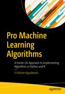
As you can see, the difference of 300 resulted in a prediction of less than 0. Similarly for a difference of –300, the prediction of linear regression will be beyond 1. However, in this case, values beyond 0 or 1 don’t make sense, because a win is a discrete value (either 0 or 1).
Hence the predictions should be bound to either 0 to 1 only—any prediction above 1 should be capped at 1 and any prediction below 0 should be floored at 0.
The fitted line
Linear regression assumes that the variables are linearly related: However, as player strength difference increases, chances of win vary exponentially.
Linear regression does not give a chance of failure: In practice, even if there is a difference of 500 points, there is an outside chance (let’s say a 1% chance) that the inferior player might win. But if capped using linear regression, there is no chance that the other player could win. In general, linear regression does not tell us the probability of an event happening after certain range.
Linear regression assumes that the probability increases proportionately as the independent variable increases: The probability of win is high irrespective of whether the rating difference is +400 or +500 (as the difference is significant). Similarly, the probability of win is low, irrespective of whether the difference is –400 or –500.
A More General Solution: Sigmoid Curve
As mentioned, the major problem with linear regression is that it assumes that all relations are linear, although in practice very few are.
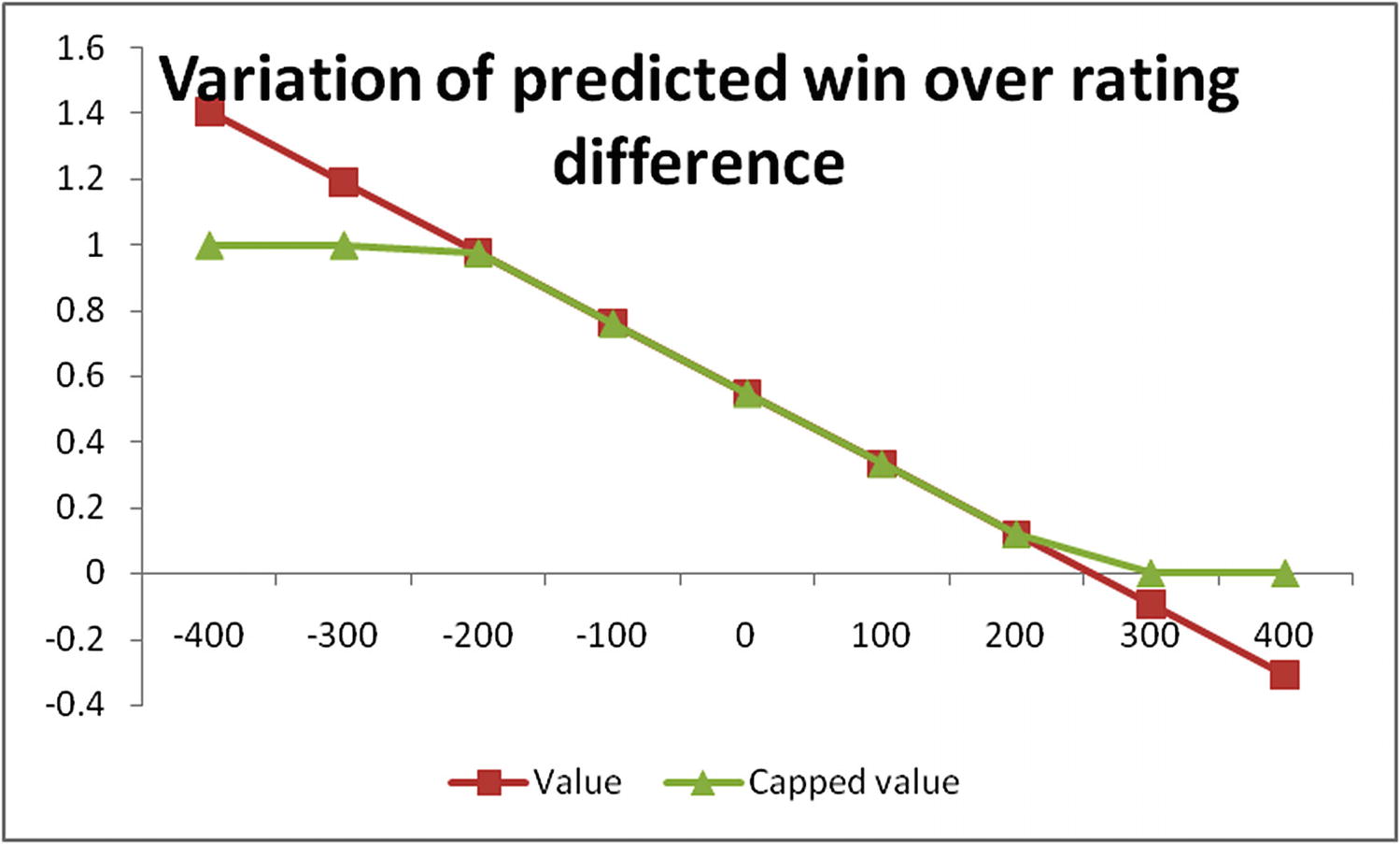
A sigmoid curve
It varies between the values 0 and 1
It plateaus after a certain threshold (after the value 3 or -3 in Figure 3-2)
The sigmoid curve would help us solve the problems faced with linear regression—that the probability of win is high irrespective of the difference in rating between white and black piece player being +400 or +500 and that the probability of win is low, irrespective of the difference being –400 or –500.
Formalizing the Sigmoid Curve (Sigmoid Activation)
We’ve seen that sigmoid curve is in a better position to explain discrete phenomenon than linear regression.
A sigmoid curve can be represented in a mathematical formula as follows:

In that equation, the higher the value of t, lower the value of  hence S(t) is close to 1. And the lower the value of t (let’s say –100), the higher the value of
  and the higher the value of (1 +
 ), hence S(t) is very close to 0.
From Sigmoid Curve to Logistic Regression
Linear regression assumes a linear relation between dependent and independent variables. It is written as Y = a + b × X. Logistic regression moves away from the constraint that all relations are linear by applying a sigmoid curve.

We can see that logistic regression uses independent variables in the same way as linear regression but passes them through a sigmoid activation so that the outputs are bound between 0 and 1.
In case of the presence of multiple independent variables, the equation translates to a multivariate linear regression passing through a sigmoid activation.
Interpreting the Logistic Regression
Linear regression can be interpreted in a straightforward way: as the value of the independent variable increases by 1 unit, the output (dependent variable) increases by b units.

If X = 0, the value of Y = 1 / (1 + exp(–(2))) = 0.88.
If X is increased by 1 unit (that is, X = 1), the value of Y is Y = 1 / (1 + exp(–(2 + 3 × 1))) = 1 / (1 + exp(–(5))) = 0.99.
As you see, the value of Y changed from 0.88 to 0.99 as X changed from 0 to 1. Similarly, if X were –1, Y would have been at 0.27. If X were 0, Y would have been at 0.88. There was a drastic change in Y from 0.27 to 0.88 when X went from –1 to 0 but not so drastic when X moved from 0 to 1.
Thus the impact on Y of a unit change in X depends on the equation.
The value 0.88 when X = 0 can be interpreted as the probability. In other words, on average in 88% of cases, the value of Y is 1 when X = 0.
Working Details of Logistic Regression
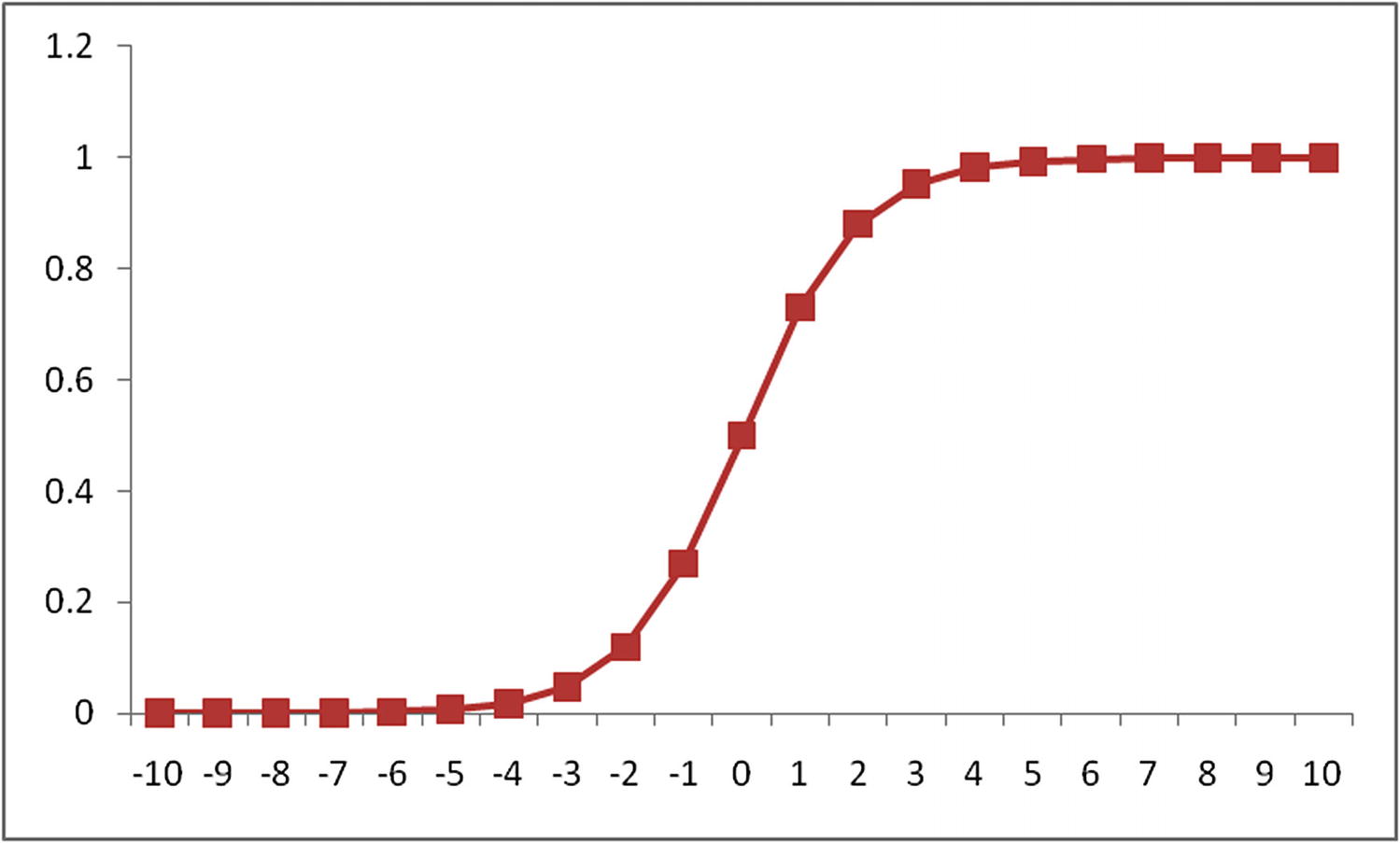
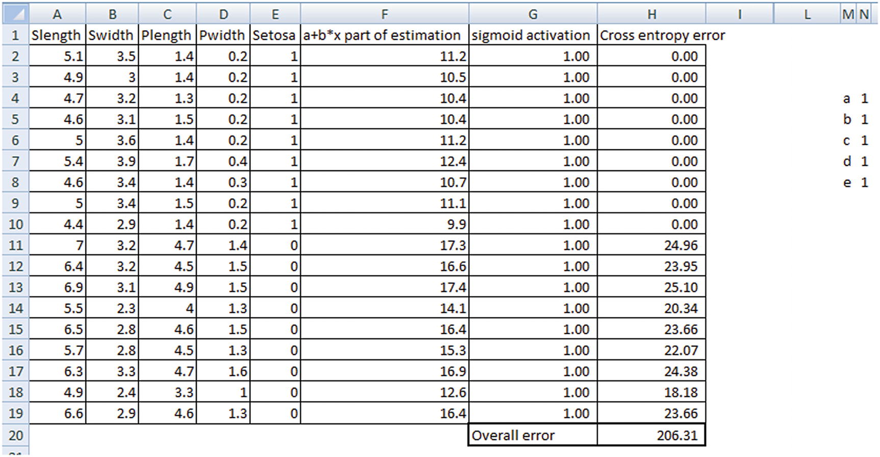
To see how a logistic regression works, we’ll go through the same exercise we did to learn linear regression in the last chapter: we’ll build a logistic regression equation in Excel. For this exercise, we’ll use the Iris dataset. The challenge is to be able to predict whether the species is Setosa or not, based on a few variables (sepal, petal length, and width).
- 1.
Initialize the weights of independent variables to random values (let’s say 1 each).
- 2.
Once the weights and the bias are initialized, we’ll estimate the output value (the probability of the species being Setosa) by applying sigmoid activation on the multivariate linear regression of independent variables.
The next table contains information about the (a + b × X) part of the sigmoid curve and ultimately the sigmoid activation value.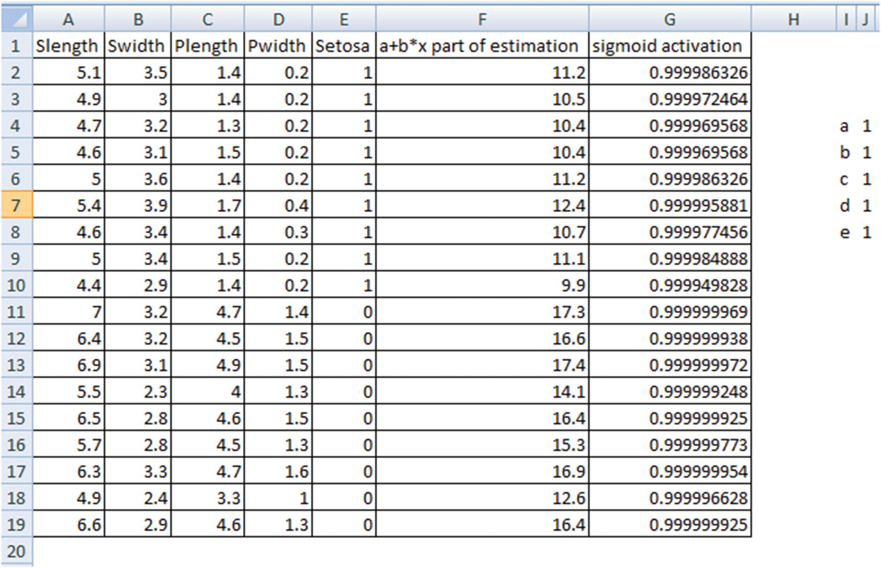 The formula for how the values in the preceding table are obtained is given in the following table:
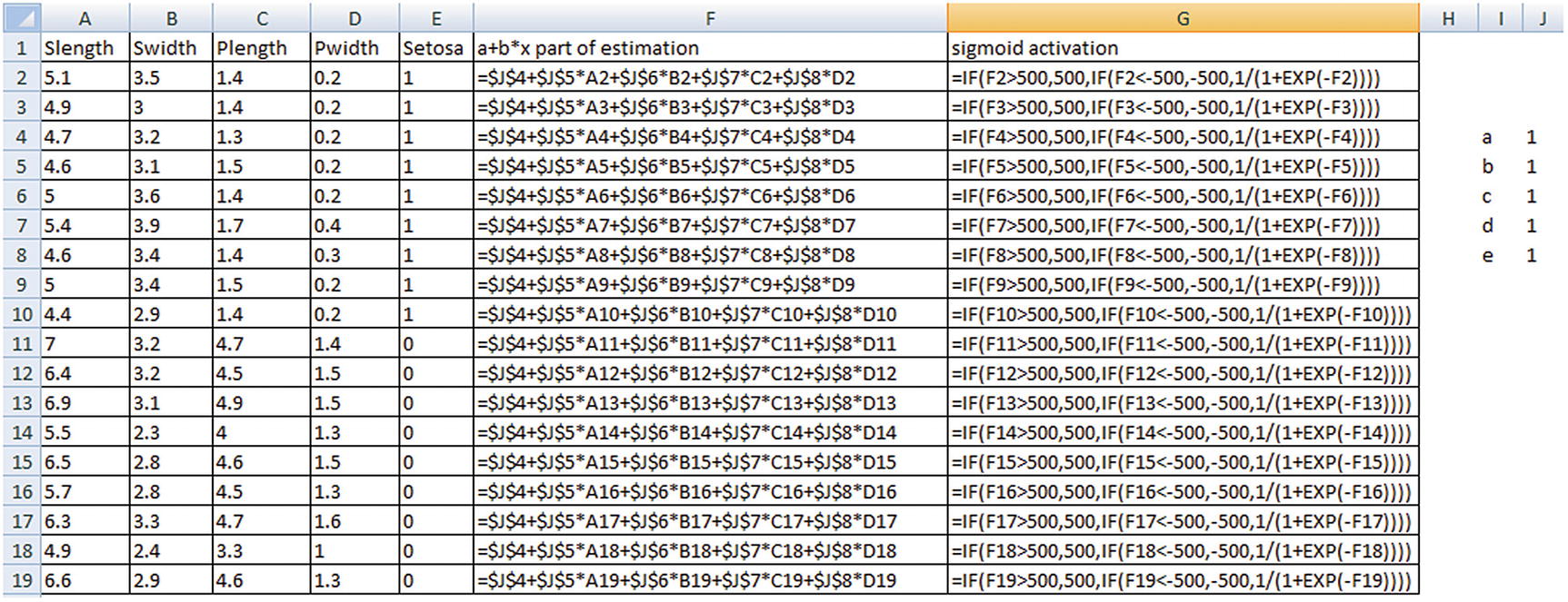
The ifelse condition in the preceding sigmoid activation column is used only because Excel has limitations in calculating any value greater than exp(500)—hence the clipping.
Estimating Error
In Chapter 2, we considered least squares (the squared difference) between actual and forecasted value to estimate overall error. In logistic regression, we will use a different error metric, called cross entropy.
Cross entropy is a measure of difference between two different distributions - actual distribution and predicted distribution. In order to understand cross entropy, let’s see an example: two parties contest in an election, where party A won. In one scenario, chances of winning are 0.5 for each party—in other words, few conclusions can be drawn, and the information is minimal. But if party A has an 80% chance of winning, and party B has a 20% chance of winning, we can draw a conclusion about the outcome of election, as the distributions of actual and predicted values are closer.

Let’s plug the two election scenarios into that equation.
Scenario 1
Model prediction for party A | Actual outcome for party A |
|---|---|
0.5 | 1 |

Scenario 2
Model prediction for party A | Actual outcome for party A |
|---|---|
0.8 | 1 |

We can see that scenario 2 has lower cross entropy when compared to scenario 1.
Least Squares Method and Assumption of Linearity
Given that in preceding example, when probability was 0.8, cross entropy was lower compared to when probability was 0.5, could we not have used least squares difference between predicted probability, actual value and proceeded in a similar way to how we proceeded for linear regression? This section discusses choosing cross entropy error over the least squares method.
A typical example of logistic regression is its application in predicting whether a cancer is benign or malignant based on certain attributes.
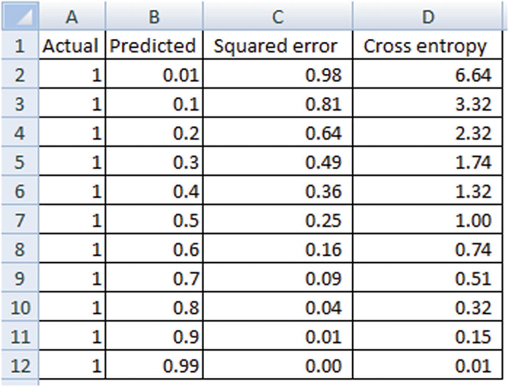
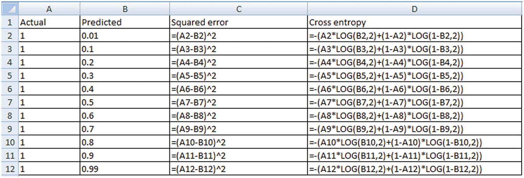
Note that cross entropy penalizes heavily for high prediction errors compared to squared error: lower error values have similar loss in both squared error and cross entropy error, but for higher differences between actual and predicted values, cross entropy penalizes more than the squared error method. Thus, we will stick to cross entropy error as our error metric, preferring it to squared error for discrete variable prediction.
Now that we have set up our problem, let’s vary the parameters in such a way that overall error is minimized. This step again is performed by gradient descent, which can be done by using the Solver functionality in Excel.
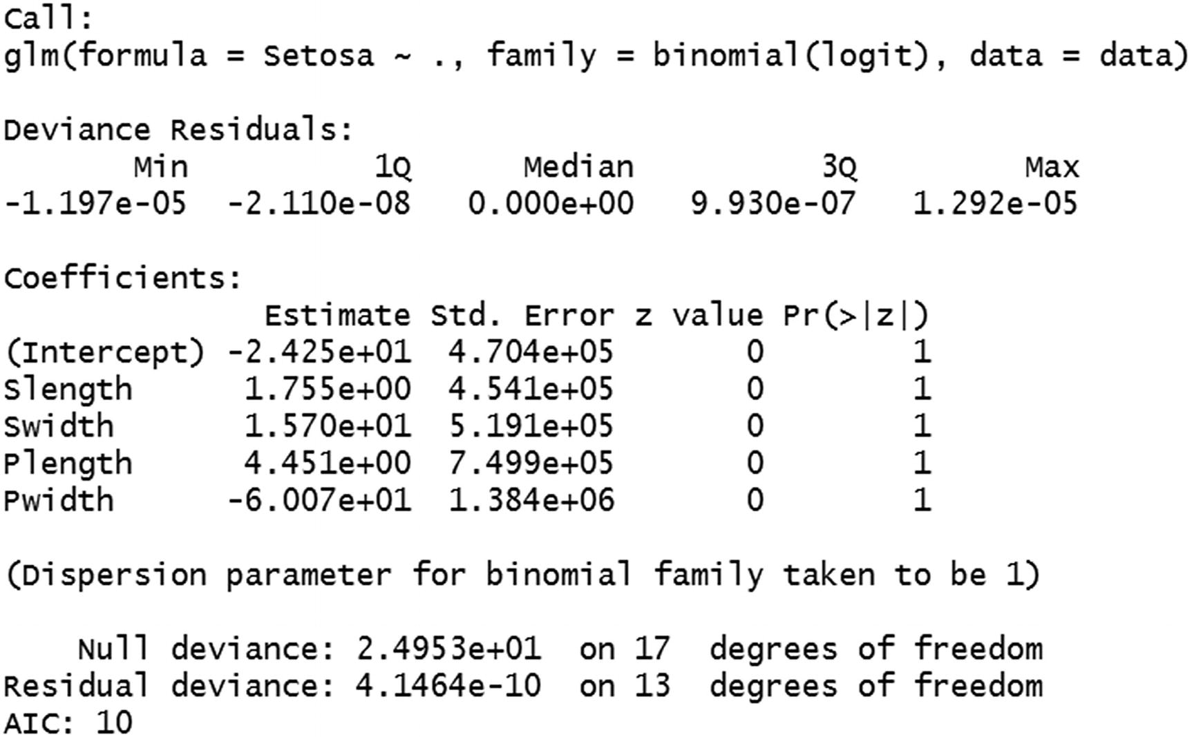
Running a Logistic Regression in R
Now that we have some background in logistic regression, we’ll dive into the implementation details of the same in R (available as “logistic regression.R” in github):
The second line in the preceding code specifies that we will be using the glm (generalized linear models), in which binomial family is considered. Note that by specifying “~.” we’re making sure that all variables are being considered as independent variables.
Running a Logistic Regression in Python
Now let’s see how a logistic regression equation is built in Python (available as “logistic regression.ipynb” in github):
The summary function in the preceding code gives a summary of the model, similar to the way in which we obtained summary results in linear regression.
Identifying the Measure of Interest
In linear regression, we have looked at root mean squared error (RMSE) as a way to measure error.
In logistic regression, the way we measure the performance of the model is different from how we measured it in linear regression. Let’s explore why linear regression error metrics cannot be used in logistic regression.
We’ll look at building a model to predict a fraudulent transaction . Let’s say 1% of the total transactions are fraudulent transactions. We want to predict whether a transaction is likely to be fraud. In this particular case, we use logistic regression to predict the dependent variable fraud transaction by using a set of independent variables.
Why can’t we use an accuracy measure? Given that only 1% of all the transactions are fraud, let’s consider a scenario where all our predictions are 0. In this scenario, our model has an accuracy of 99%. But the model is not at all useful in reducing fraudulent transactions because it predicts that every transaction is not a fraud.
In a typical real-world scenario, we would build a model that predicts whether the transaction is likely to be a fraud or not, and only the transactions that have a high likelihood of fraud are flagged. The transactions that are flagged are then sent for manual review to the operations team, resulting in a lower fraudulent transaction rate.
Although we are reducing the fraud transaction rate by getting the high-likelihood transactions reviewed by the operations team, we are incurring an additional cost of manpower, because humans are required to review the transaction.
A fraud transaction prediction model can help us narrow the number of transactions that need to be reviewed by a human (operations team). Let’s say in total there are a total of 1,000,000 transactions. Of those million transactions, 1% are fraudulent—so, a total of 10,000 transactions are fraudulent.
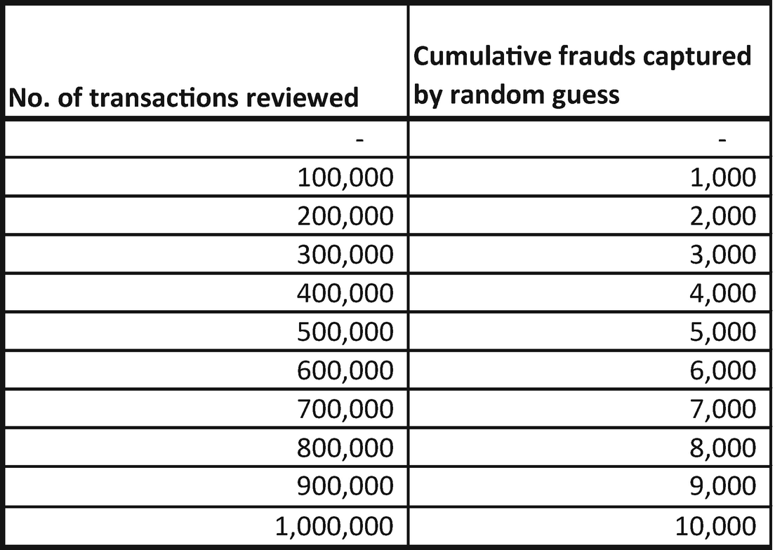
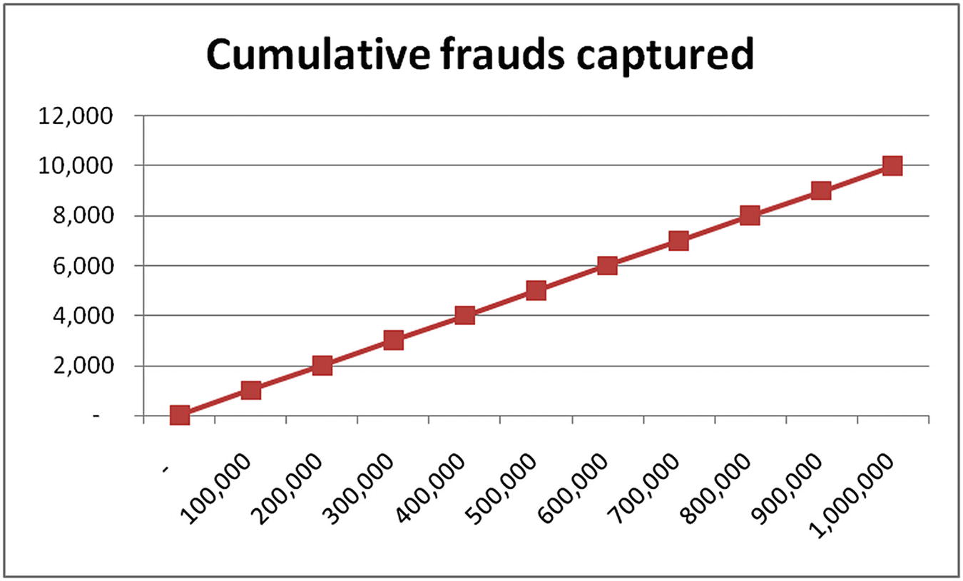
Cumulative frauds captured by random guess model
- 1.Take the dataset as input and compute the probabilities of each transaction id:
Transaction id
Actual fraud
Probability of fraud
1
1
0.56
2
0
0.7
3
1
0.39
4
1
0.55
5
1
0.03
6
0
0.84
7
0
0.05
8
0
0.46
9
0
0.86
10
1
0.11
- 2.Sort the dataset by probability of fraud from the highest to least. The intuition is that the model performs well when there are more 1s of “Actual fraud” at the top of dataset after sorting in descending order by probability:
Transaction id
Actual fraud
Probability of fraud
9
0
0.86
6
0
0.84
2
0
0.7
1
1
0.56
4
1
0.55
8
0
0.46
3
1
0.39
10
1
0.11
7
0
0.05
5
1
0.03
- 3.Calculate the cumulative number of transactions captured from the sorted table:
Transaction id
Actual fraud
Probability of fraud
Cumulative transactions reviewed
Cumulative frauds captured
9
0
0.86
1
0
6
0
0.84
2
0
2
0
0.7
3
0
1
1
0.56
4
1
4
1
0.55
5
2
8
0
0.46
6
2
3
1
0.39
7
3
10
1
0.11
8
4
7
0
0.05
9
4
5
1
0.03
10
5
Transaction id | Actual fraud | Cumulative transactions reviewed | Cumulative frauds captured | Cumulative frauds captured by random guess |
|---|---|---|---|---|
9 | 0 | 1 | 0 | 0.5 |
6 | 0 | 2 | 0 | 1 |
2 | 0 | 3 | 0 | 1.5 |
1 | 1 | 4 | 1 | 2 |
4 | 1 | 5 | 2 | 2.5 |
8 | 0 | 6 | 2 | 3 |
3 | 1 | 7 | 3 | 3.5 |
10 | 1 | 8 | 4 | 4 |
7 | 0 | 9 | 4 | 4.5 |
5 | 1 | 10 | 5 | 5 |
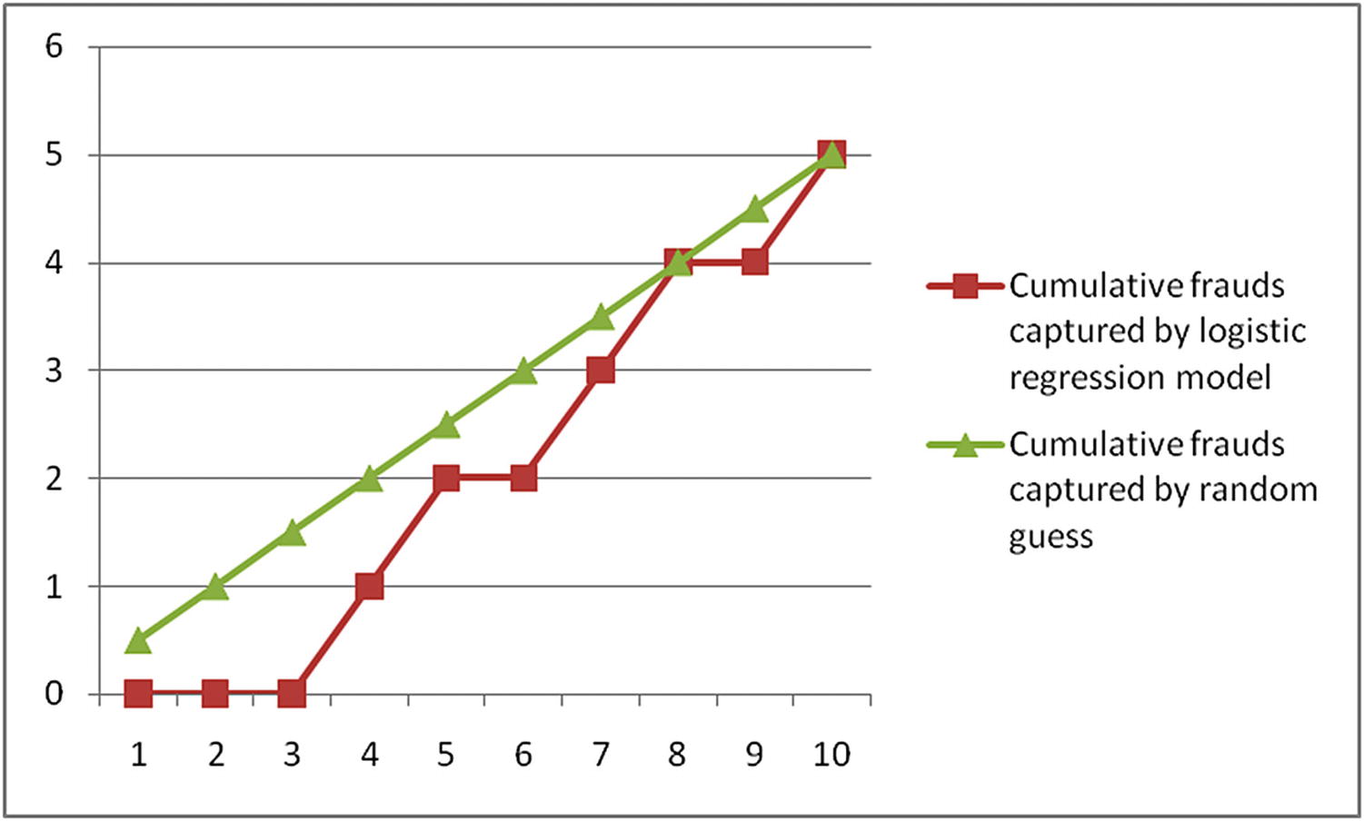
Comparing the models
In this particular case, for the example laid out above, random guess turned out to be better than the logistic regression model—in the first few guesses, a random guess makes better predictions than the model.
Cumulative frauds captured | ||
|---|---|---|
No. of transactions reviewed | Cumulative frauds captured by random guess | Cumulative frauds captued by model |
- | - | 0 |
100,000 | 1,000 | 4000 |
200,000 | 2,000 | 6000 |
300,000 | 3,000 | 7600 |
400,000 | 4,000 | 8100 |
500,000 | 5,000 | 8500 |
600,000 | 6,000 | 8850 |
700,000 | 7,000 | 9150 |
800,000 | 8,000 | 9450 |
900,000 | 9,000 | 9750 |
1,000,000 | 10,000 | 10000 |
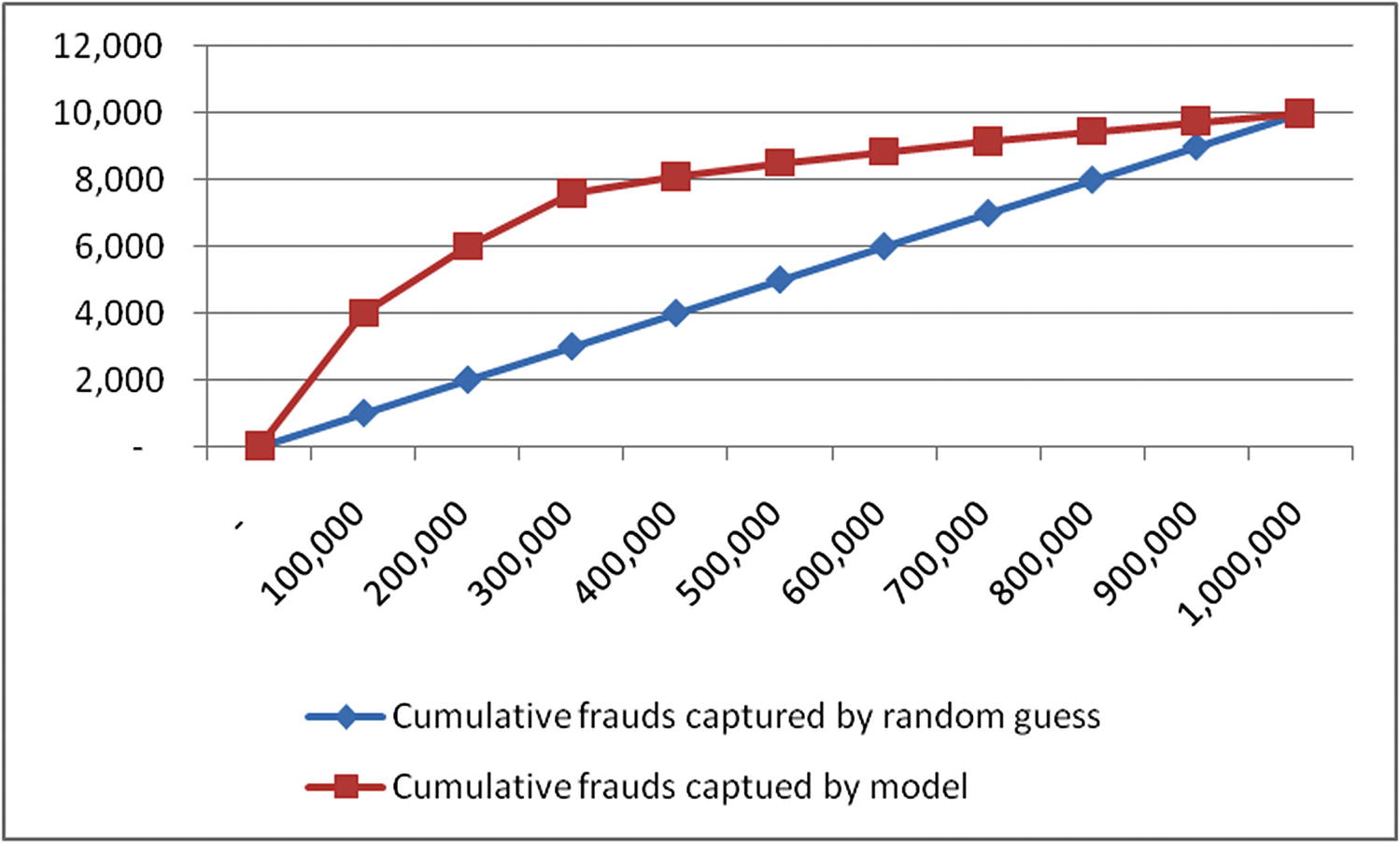
Comparing the two approaches
Note that the higher the area between the random guess line and the model line, the better the model performance is. The metric that measures the area covered under model line is called the area under the curve (AUC) .
Thus, the AUC metric is a better metric to helps us evaluate the performance of a logistic regression model .
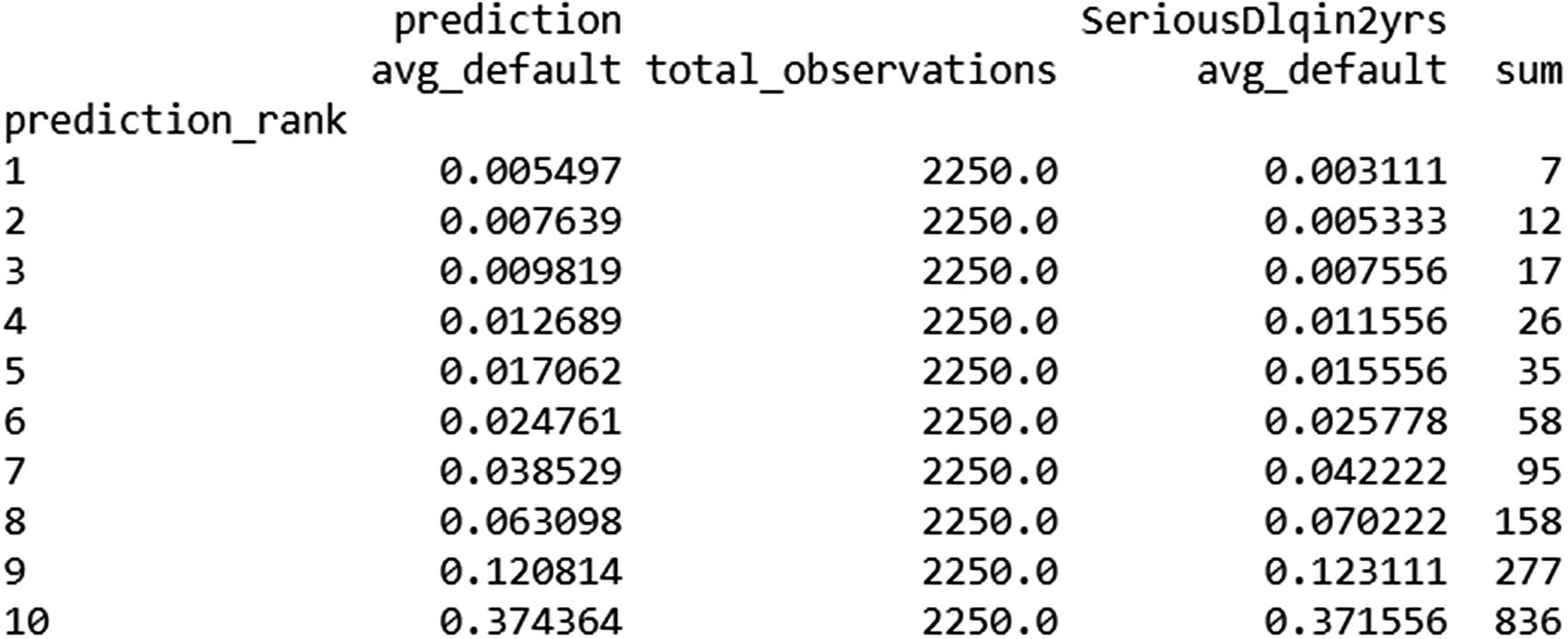
prediction_rank in the preceding table represents the decile of probability—that is, after each transaction is rank ordered by probability and then grouped into buckets based on the decile it belongs to. Note that the third column (total_observations) has an equal number of observations in each decile.
The second column—prediction avg_default—represents the average probability of default obtained by the model we built. The fourth column—SeriousDlqin2yrs avg_default—represents the average actual default in each bucket. And the final column represents the actual number of defaults captured in each bucket.
Note that in an ideal scenario, all the defaults should be captured in the highest-probability buckets. Also note that, in the preceding table, the model captured considerable number of frauds in the highest probability bucket.
Common Pitfalls
This section talks about some the common pitfalls the analyst should be careful about while building a classification model:
Time Between Prediction and the Event Happening
Let’s look at a case study: predicting the default of a customer.
We should say that it is useless to predict today that someone is likely to default on their credit card tomorrow. There should be some time gap between the time of predicting that someone would default and the event actually happening. The reason is that the operations team would take some time to intervene and help reduce the number of default transactions.
Outliers in Independent variables
Similar to how outliers in the independent variables impact the overall error in linear regression, it is better to cap outliers so that they do not impact the regression very much in logistic regression. Note that, unlike linear regression, logistic regression would not have a huge outlier output when one has an outlier input; in logistic regression, the output is always restricted between 0 and 1 and the corresponding cross entropy loss associated with it.
But the problem with having outliers would still result in a high cross entropy loss, and so it’s a better idea to cap outliers.
Summary
Logistic regression is used in predicting binary (categorical) events, and linear regression is used to forecast continuous events.
Logistic regression is an extension of linear regression, where the linear equation is passed through a sigmoid activation function.
One of the major loss metrics used in logistic regression is the cross entropy error.
A sigmoid curve helps in bounding the output of a value between 0 to 1 and thus in estimating the probability associated with an event.
AUC metric is a better measure of evaluating a logistic regression model.