Regression typically works best when the ratio of number of data points to number of variables is high. However, in some scenarios, such as clinical trials, the number of data points is limited (given the difficulty in collecting samples from many individuals), and the amount of information collected is high (think of how much information labs give us based on small samples of collected blood).
There is a high chance that a majority of the variables are correlated to each other.
The time taken to run a regression could be very extensive because the number of weights that need to be predicted is large.
Techniques like principal component analysis (PCA) come to the rescue in such cases. PCA is an unsupervised learning technique that helps in grouping multiple variables into fewer variables without losing much information from the original set of variables.
In this chapter, we will look at how PCA works and get to know the benefits of performing PCA. We will also implement it in Python and R.
Intuition of PCA
Dep Var | Var 1 | Var 2 |
|---|---|---|
0 | 1 | 10 |
0 | 2 | 20 |
0 | 3 | 30 |
0 | 4 | 40 |
0 | 5 | 50 |
1 | 6 | 60 |
1 | 7 | 70 |
1 | 8 | 80 |
1 | 9 | 90 |
1 | 10 | 100 |
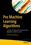
We’ll assume both Var 1 and Var 2 are the independent variables used to predict the dependent variable (Dep Var). We can see that Var 2 is highly correlated to Var 1, where Var 2 = (10) × Var 1.
A plot of their relation can be seen in Figure 12-1.
Plotting the relation
In the figure, we can clearly see that there is a strong relation between the variables. This means the number of independent variables can be reduced.
The equation can be expressed like this:
Var2 = 10 × Var1
In other words, instead of using two different independent variables, we could have just used one variable Var1 and it would have worked out in solving the problem.
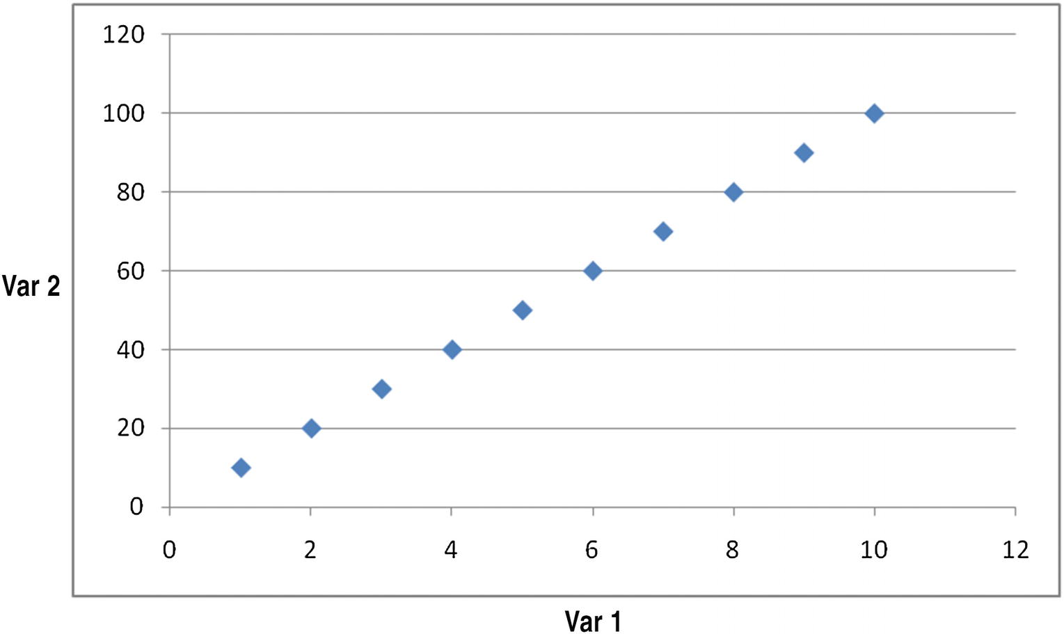
Moreover, if we are in a position to view the two variables through a slightly different angle (or, we rotate the dataset), like the one indicated by the arrow in Figure 12-2, we see a lot of variation in horizontal direction and very little in vertical direction.
Viewpoint/angle from which data points should be looked at
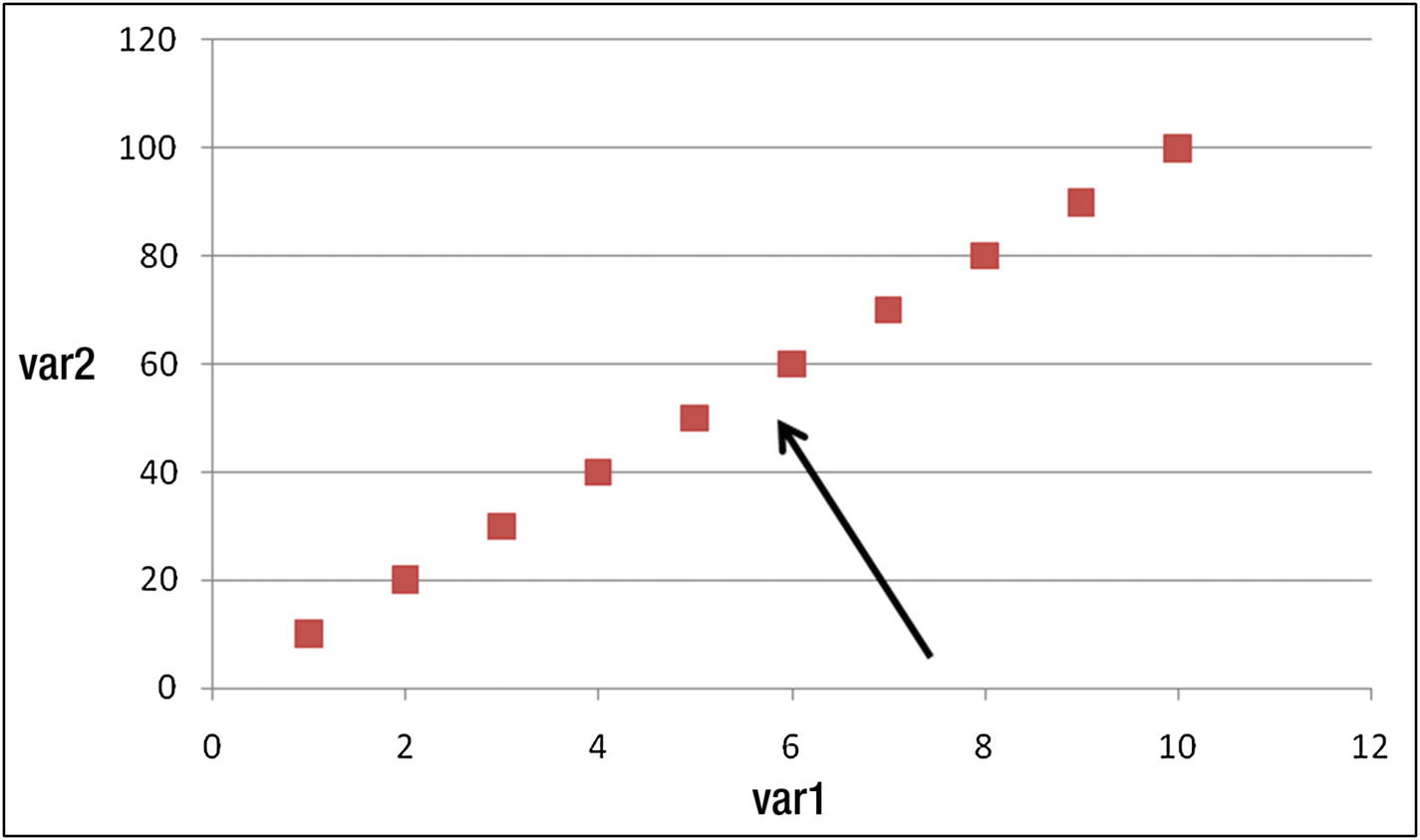
Let’s complicate our dataset by a bit. Consider a case where the relation between v1 and v2 is like that shown in Figure 12-3.
Plotting two variables
Again, the two variables are highly correlated with each other, though not as perfectly correlated as the previous case.
In such scenario, the first principle component is the line/variable that explains the maximum variance in the dataset and is a linear combination of multiple independent variables. Similarly, the second principal component is the line that is completely uncorrelated (has a correlation of close to 0) to the first principal component and that explains the rest of variance in dataset, while also being a linear combination of multiple independent variables.
Typically the second principal component is a line that is perpendicular to the first principal component (because the next highest variation happens in a direction that is perpendicular to the principal component line).
In general, the nth principal component of a dataset is perpendicular to the (n – 1)th principal component of the same dataset.
Working Details of PCA
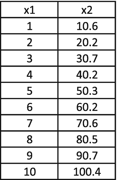
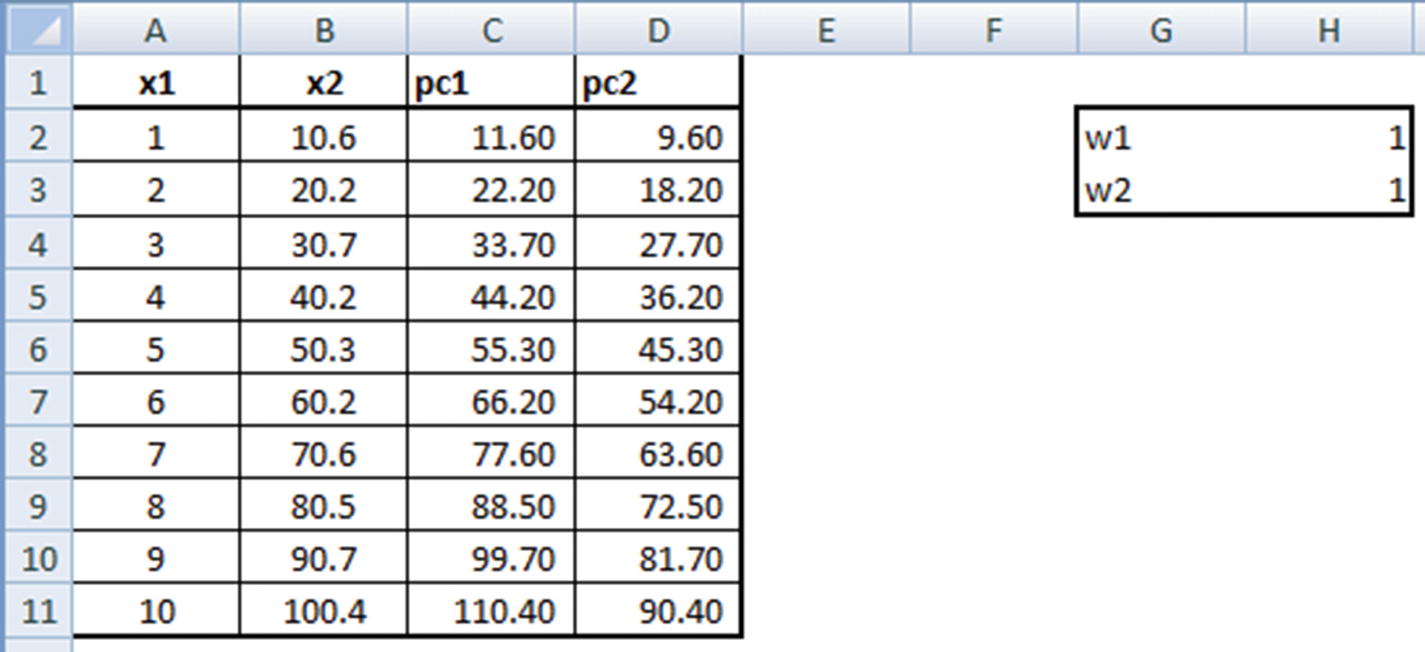
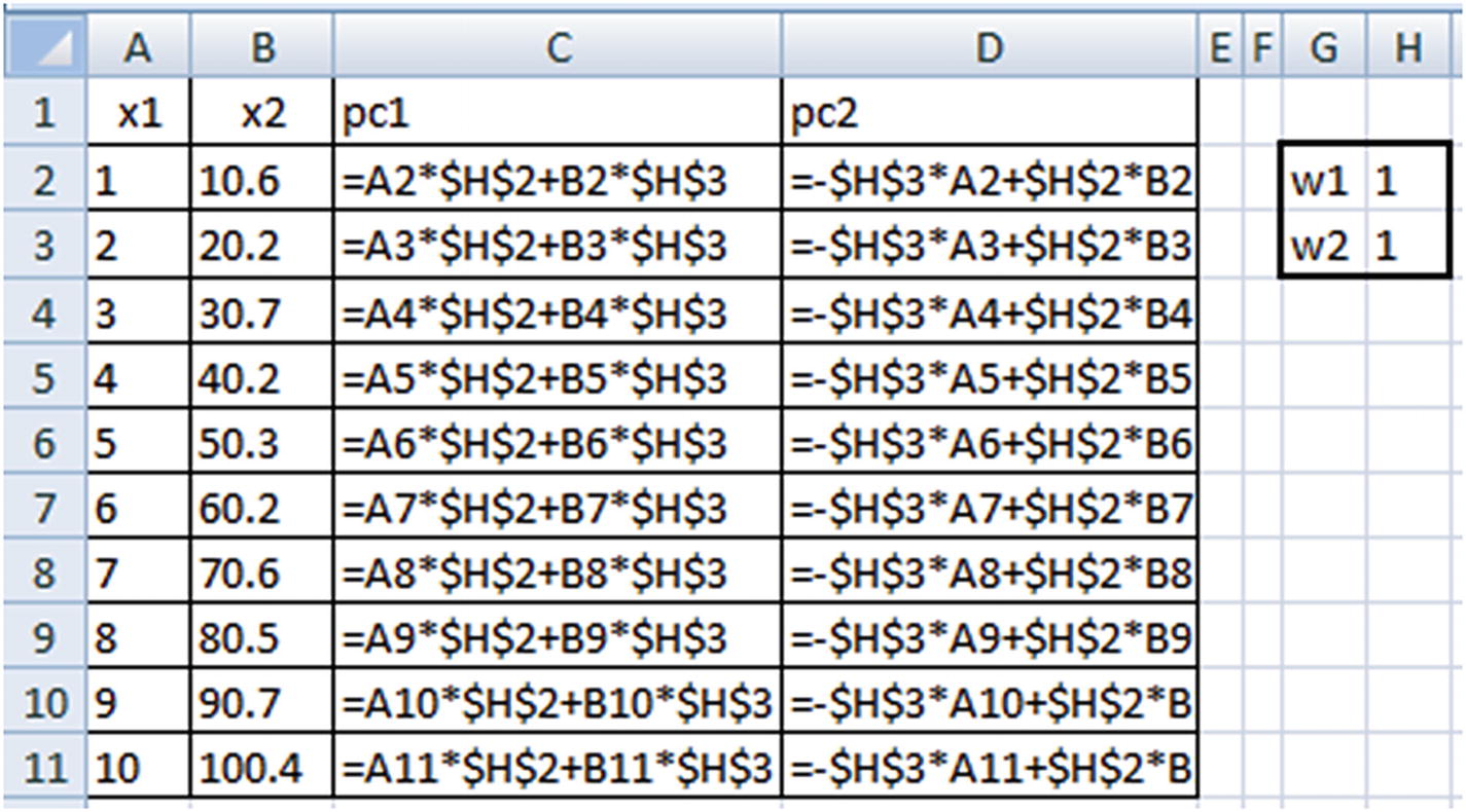
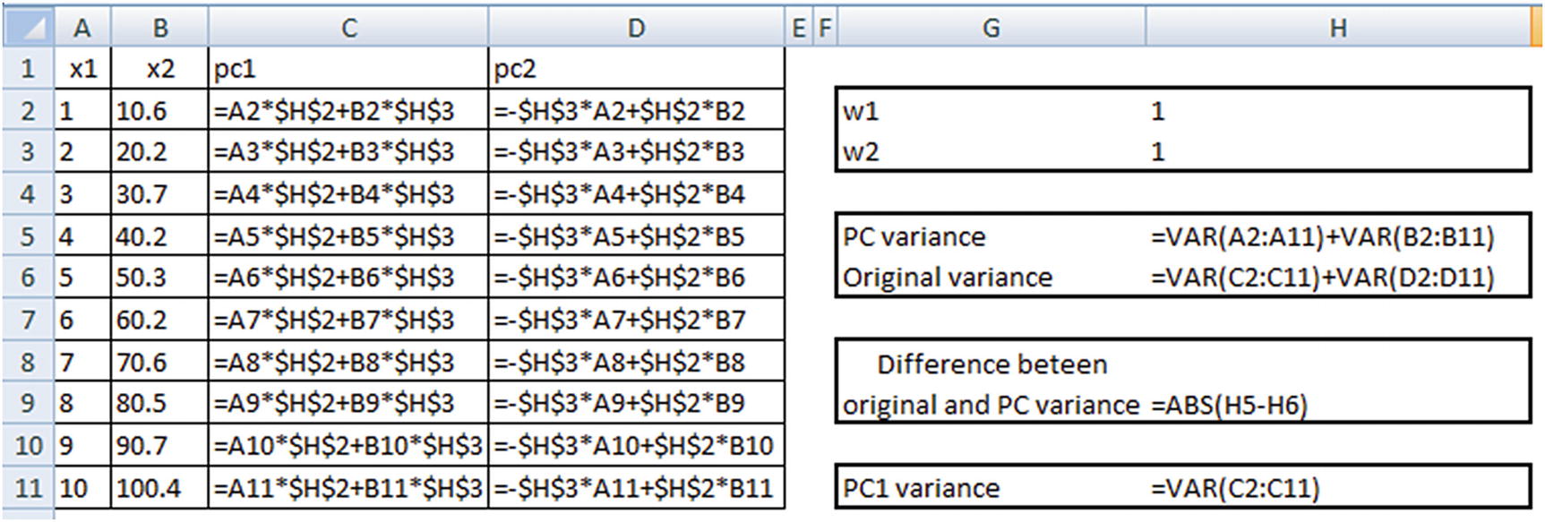
Given that a principal component is a linear combination of variables, we’ll express it as follows:
PC1 = w1 × x1 + w2 × x2
Similarly, the second principal component is perpendicular to the original line, as follows:
PC2 = –w2 × x1 + w1 × x2
The weights w1 and w2 are randomly initialized and should be iterated further to obtain the optimal ones.
Objective: Maximize PC1 variance.
Constraint: Overall variance in principal components should be equal to the overall variance in original dataset (as the data points did not change, but only the angle from which we view the data points changed).
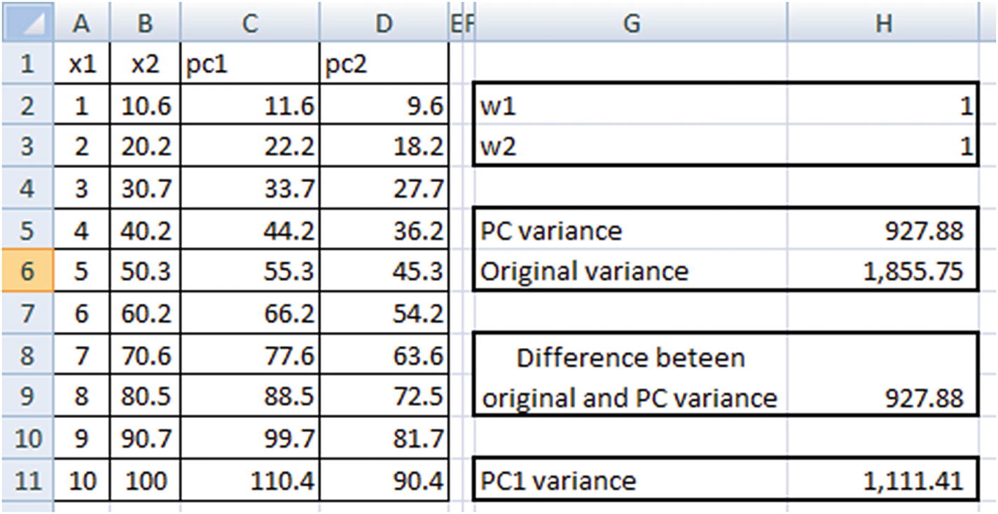
Note that PC variance = PC1 variance + PC2 variance.
Original variance = x1 variance + x2 variance
Once the dataset is initialized, we will proceed with identifying the optimal values of w1 and w2 that satisfy our objective and constraint.
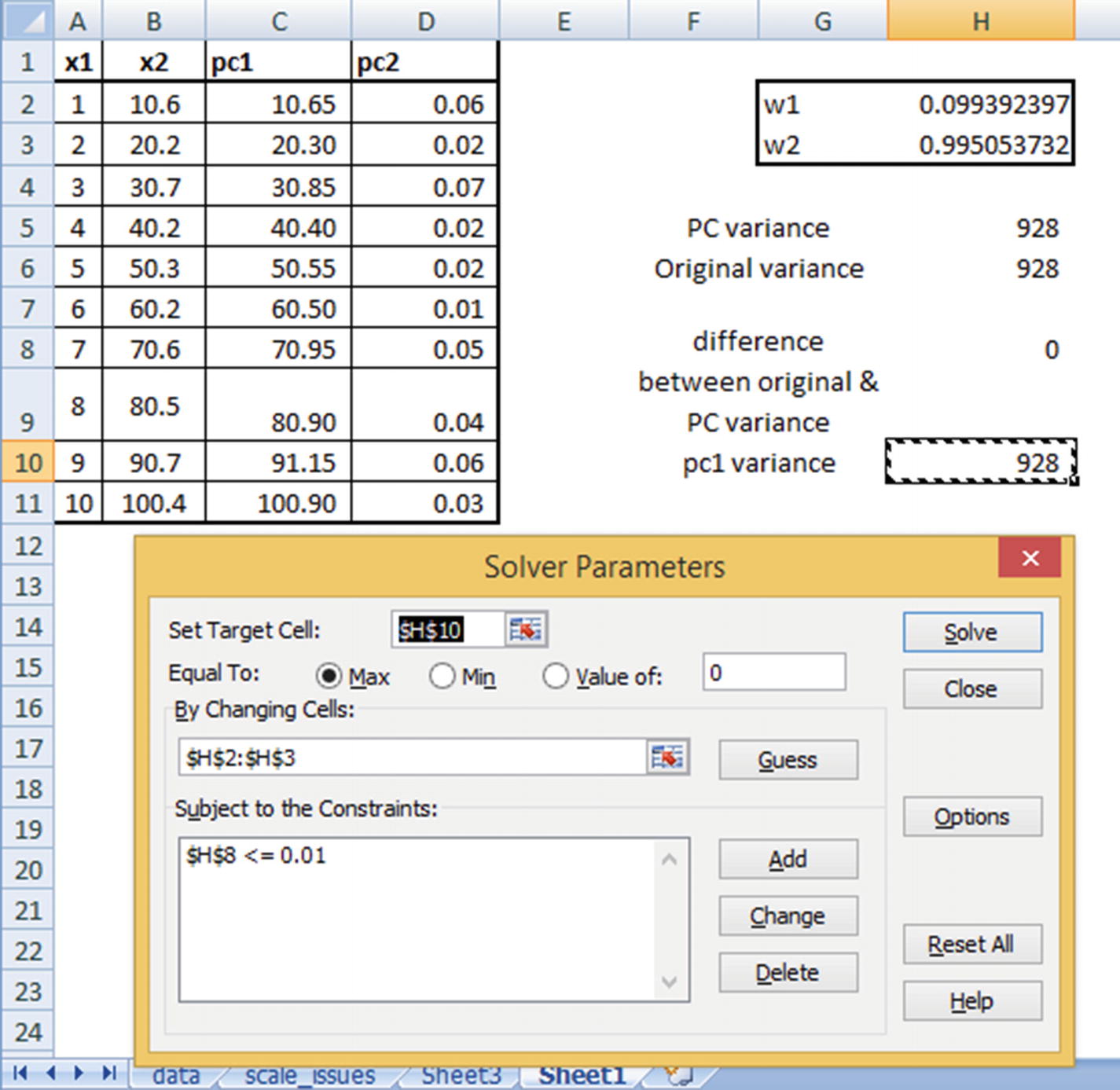
PC1 variance is maximized.
There is hardly any difference between the original dataset variance and the principal component dataset variance. (We have allowed for a small difference of less than 0.01 only so that Excel is able to solve it because there may be some rounding-off errors.)
Note that PC1 and PC2 are now highly uncorrelated with each other, and PC1 explains the highest variance across all variables. Moreover, x2 has a higher weightage in determining PC1 than x1 (as is evident from the derived weight values).
Scaling Data in PCA
One of the major pre-processing steps in PCA is to scale the variables. Consider the following scenario: we are performing PCA on two variables. One variable has a range of values from 0–100, and another variable has a range of values from 0–1.
Given that, using PCA, we are trying to capture as much variation in the dataset as possible, the first principal component will give a very high weightage to the variable that has maximum variance (in our case, Var1) when compared to the variable with low variance.
Hence, when we work out w1 and w2 for the principal component, we will end up with a w1 that is close to 0 and a w2 that is close to 1 (where w2 is the weight in PC1 corresponding to the higher ranged variable). To avoid this, it is advisable to scale each variable so that both of them have similar range, due to which variance can be comparable.
Extending PCA to Multiple Variables
So far, we have seen building a PCA where there are two independent variables. In this section, we will consider how to hand-build a PCA where there are more than two independent variables.
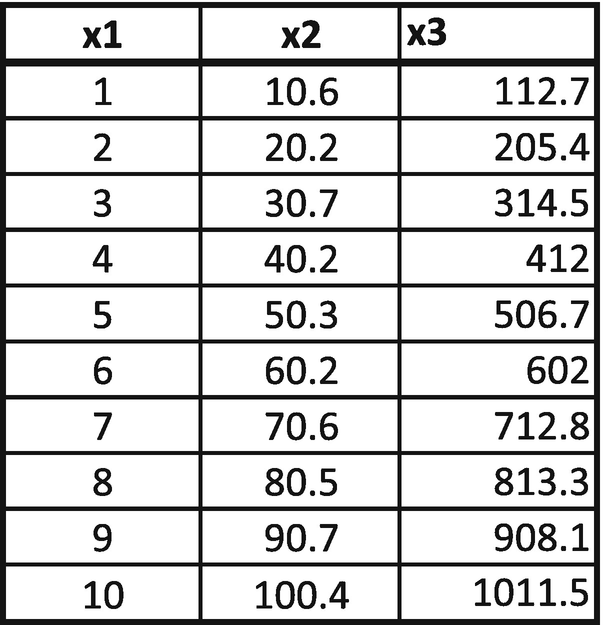
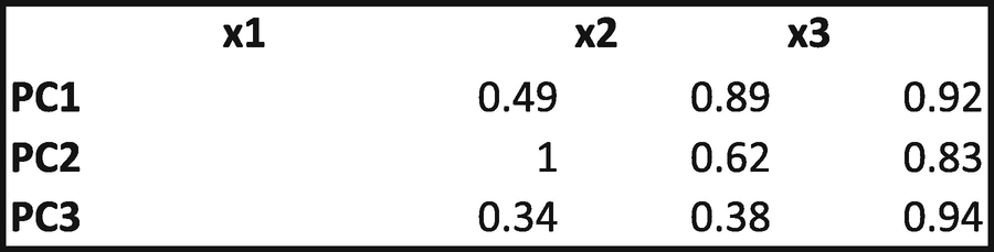
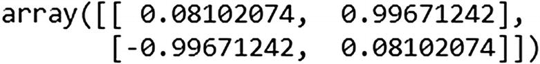
From this matrix, we can consider PC1 = 0.49 × x1 + 0.89 × x2 + 0.92 × x3. PC2 and PC3 would be worked out similarly. If there were four independent variables, we would have had a 4 × 4-weight matrix.
Objective: Maximize PC1 variance.
Constraints: Overall PC variance should be equal to overall original dataset variance. PC1 variance should be greater than PC2 variance, PC1 variance should be greater than PC3 variance, and PC2 variance should be greater than PC3 variance.
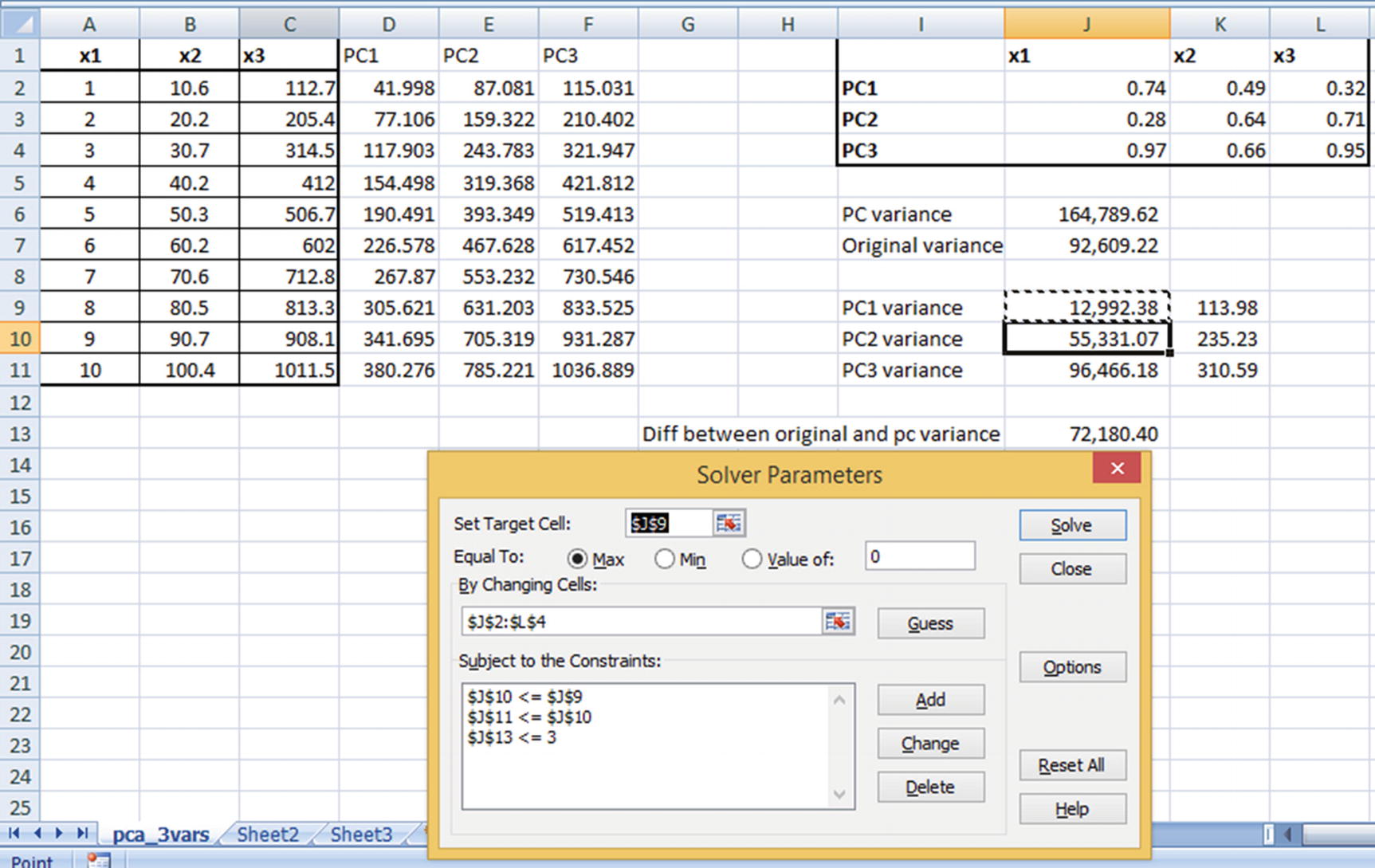
Solving for the preceding would result in the optimal weight combination that satisfies our criterion. Note that the output from Excel could be slightly different from the output you would see in Python or R, but the output of Python or R is likely to have higher PC1 variance when compared to the output of Excel, due to the underlying algorithm used in solving. Also note that, even though ideally we would have wanted the difference between original and PC variance to be 0, for practical reasons of executing the optimization using Excel solver we have allowed the difference to be a maximum of 3.
Similar to the scenario of the PCA with two independent variables, it is a good idea to scale the inputs before processing PCA. Also, note that PC1 explains the highest variation after solving for the weights, and hence PC2 and PC3 can be eliminated because they explain very little of the original dataset variance.
Choosing the Number of Principal Components to Consider
There is no single prescribed method to choosing the number of principal components. In practice, a rule of thumb is to choose the minimum number of principal components that cumulatively explain 80% of the total variance in the dataset.
Implementing PCA in R
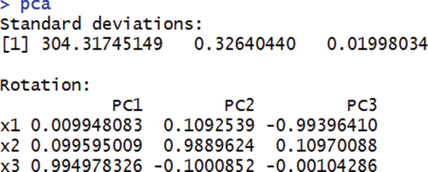
The standard deviation values here are the same as the standard deviation values of PC variables. The rotation values are the same as the weight values that we initialized earlier.
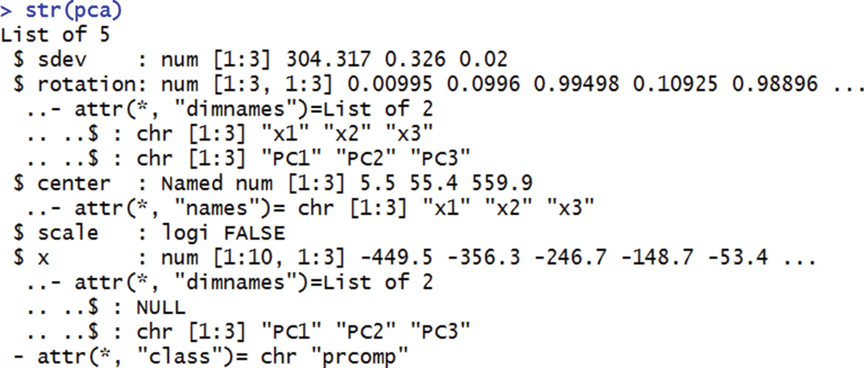
From this, we notice that apart from the standard deviation of PC variables and the weight matrix, pca also provides the transformed dataset.
We can access the transformed dataset by specifying pca$x.
Implementing PCA in Python
We see that we fit as many components as the number of independent variables and fit PCA on top of the data.

explained_variance_ratio_ provides the amount of variance explained by each principal component. This is very similar to the standard deviation output in R, where R gives us the standard deviation of each principal component. PCA in Python’s scikit learn transformed it slightly and gave us the amount of variance out of the original variance explained by each variable.
Applying PCA to MNIST
MNIST is a handwritten digit recognition task. A 28 × 28 image is unrolled, where each pixel value is represented in a column. Based on that, one is expected to predict if the output is one of the numbers between 0 and 9.
Columns with zero variance
Columns with very little variance
Columns with high variance
In a way, PCA helps us in eliminating low- and no-variance columns as much as possible while still achieving decent accuracy with a limited number of columns.
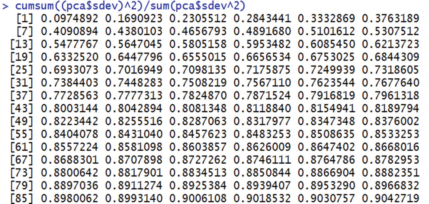
From this we can see that the first 43 principal components explain ~80% of the total variance in the original dataset. Instead of running a model on all 784 columns, we could run the model on the first 43 principal components without losing much information and hence without losing out much on accuracy.
Summary
PCA is a way of reducing the number of independent variables in a dataset and is particularly applicable when the ratio of data points to independent variables is low.
It is a good idea to scale independent variables before applying PCA.
PCA transforms a linear combination of variables such that the resulting variable expresses the maximum variance within the combination of variables.