V Kishore AyyadevaraPro Machine Learning Algorithms https://doi.org/10.1007/978-1-4842-3564-5_6

6. Gradient Boosting Machine

V Kishore Ayyadevara¹

(1)

Hyderabad, Andhra Pradesh, India

So far, we’ve considered decision trees and random forest algorithms. We saw that random forest is a bagging (bootstrap aggregating) algorithm—it combines the output of multiple decision trees to give the prediction. Typically, in a bagging algorithm trees are grown in parallel to get the average prediction across all trees, where each tree is built on a sample of original data.

Gradient boosting , on the other hand, does the predictions using a different format. Instead of parallelizing the tree building process, boosting takes a sequential approach to obtaining predictions. In gradient boosting, each decision tree predicts the error of the previous decision tree—thereby boosting (improving) the error (gradient).

In this chapter, you will learn the following:

Working details of gradient boosting
How gradient boosting is different from random forest
The working details of AdaBoost
The impact of various hyper-parameters on boosting
How to implement gradient boosting in R and Python

Gradient Boosting Machine

Gradient refers to the error, or residual, obtained after building a model. Boosting refers to improving. The technique is known as gradient boosting machine, or GBM. Gradient boosting is a way to gradually improve (reduce) error.

To see how GBM works, let’s begin with an easy example. Assume you’re given a model M (which is based on decision tree) to improve upon. Let’s say the current model accuracy is 80%. We want to improve on that.

We’ll express our model as follows:

Y = M(x) + error

Y is the dependent variable and M(x) is the decision tree using the x independent variables.

Now we’ll predict the error from the previous decision tree:

error = G(x) + error2

G(x) is another decision tree that tries to predict the error using the x independent variables.

In the next step, similar to the previous step, we build a model that tries to predict error2 using the x independent variables:

error2 = H(x) + error3

Now we combine all these together:

Y = M(x) + G(x) + H(x) + error3

The preceding equation is likely to have an accuracy that is greater than 80% as individually model M (single decision tree) had 80% accuracy, while in the above equation we are considering 3 decision trees.

The next section explores the working details of how GBM works. In a later section, we will see how an AdaBoost (adaptive boosting) algorithm works.

Working details of GBM

Here’s the algorithm for gradient boosting:

1.
Initialize predictions with a simple decision tree.
2.
Calculate residual - which is the (actual-prediction) value.
3.
Build another shallow decision tree that predicts residual based on all the independent values.
4.
Update the original prediction with the new prediction multiplied by learning rate.
5.
Repeat steps 2 through 4 for a certain number of iterations (the number of iterations will be the number of trees).

Code implementing the preceding algorithm is as follows (code and dataset available in github as “GBM working details.ipynb”):

import pandas as pd

# importing dataset

data=pd.read_csv('F:/course/Logistic regression/credit_training.csv')

# removing irrelevant variables

data=data.drop(['Unnamed: 0'],axis=1)

# replacing null values

data['MonthlyIncome']=data['MonthlyIncome'].fillna(value=data['MonthlyIncome'].median())

data['NumberOfDependents']=data['NumberOfDependents'].fillna(value=data['NumberOfDependents'].median())

from sklearn.model_selection import train_test_split

# creating independent variables

X = data.drop('SeriousDlqin2yrs',axis=1)

# creating dependent variables

y = data['SeriousDlqin2yrs']

# creating train and test datasets

X_train, X_test, y_train, y_test = train_test_split(X, y, test_size=0.30, random_state=42)

In the preceding code, we have split the dataset into 70% training and 30% test dataset.

# Build a decision tree

from sklearn.tree import DecisionTreeClassifier

depth_tree = DecisionTreeClassifier(criterion = "gini",max_depth=4, min_samples_leaf=10)

depth_tree.fit(X_train, y_train)

In the preceding code, we are building a simple decision tree on the original data with SeriousDlqin2yrs as dependent variable and the rest of the variables as independent variables.

#Get the predictions on top of train dataset itself

dt_pred = depth_tree.predict_proba(X_train)

X_train['prediction']=dt_pred[:,1]

In the preceding code, we are predicting the outputs of the first decision tree. This will help us in coming up with the residuals.

#Get the predictions on top of test dataset

X_test['prediction']=depth_tree.predict_proba(X_test)[:,1]

In the preceding code, though we calculate the output probabilities in the test dataset, note that we are not in a position to calculate residuals because, as a practical matter, we are not allowed to peek into the dependent variable of the test dataset. As a continuation to the preceding code, we will be build 20 decision trees of residuals in the following code:

from sklearn.tree import DecisionTreeRegressor

import numpy as np

from sklearn.metrics import roc_auc_score

depth_tree2 = DecisionTreeRegressor(criterion = "mse",max_depth=4, min_samples_leaf=10)

for i in range(20):

# Calculate residual

train_errorn=y_train-X_train['prediction']

# remove prediction variable that got appended to independent variable earlier

X_train2=X_train.drop(['prediction'],axis=1)

X_test2=X_test.drop(['prediction'],axis=1)

In the preceding code, note that we are calculating the residual of the nth decision tree. We are dropping the prediction column from the X_train2 dataset because the prediction column cannot be one of the independent variables in the subsequent model that gets built in the next iteration of the for loop.

# Build a decision tree to predict the residuals using independent variables

dt2=depth_tree2.fit(X_train2, train_errorn)

# predict the residual

dt_pred_train_errorn = dt2.predict(X_train2)

In the preceding code, we are fitting the decision tree where the dependent variable is the residual and the independent variables are the original independent variables of the dataset.

Once the decision tree is fit, the next step is to predict the residual (which was the dependent variable):

# update the predictions based on predicted residuals

X_train['prediction']=(X_train['prediction']+dt_pred_train_errorn*1)

# Calculate AUC

train_auc=roc_auc_score(y_train,X_train['prediction'])

print("AUC on training data set is: "+str(train_auc))

In that code, the original predictions (which are stored in the X_train dataset) are updated with the predicted residuals we obtained in the previous step.

Note that we are updating our predictions by the prediction of residual (dt_pred_train_errorn). We have explicitly given a *1 in the preceding code because the concept of shrinkage or learning rate will be explained in the next section (the *1 will be replaced by *learning_rate).

Once the predictions are updated, we calculate the AUC on the training dataset:

# update the predictions based on predicted residuals for test dataset

dt_pred_test_errorn = dt2.predict(X_test2)

X_test['prediction']=(X_test['prediction']+dt_pred_test_errorn)

# Calculate AUC

test_auc=roc_auc_score(y_test,X_test['prediction'])

print("AUC on test data set is: "+str(test_auc))

Here we update the predictions on the test dataset. We do not know the residuals of test dataset, but we update predictions on the test dataset on the basis of the decision tree that got built to predict the residuals of the training dataset. Ideally, if the test dataset has no residuals, the predicted residuals should be close to 0, and if the original decision tree of the test dataset had some residuals, then the predicted residuals would be away from 0.

Once the predictions of the test dataset are updated, we print out the AUC of the test dataset.

Let’s look at the output of the preceding code:

../images/463052_1_En_6_Chapter/463052_1_En_6_Figa_HTML.jpg

../images/463052_1_En_6_Chapter/463052_1_En_6_Figb_HTML.jpg

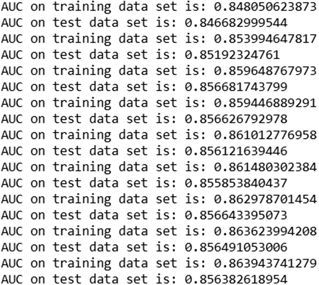
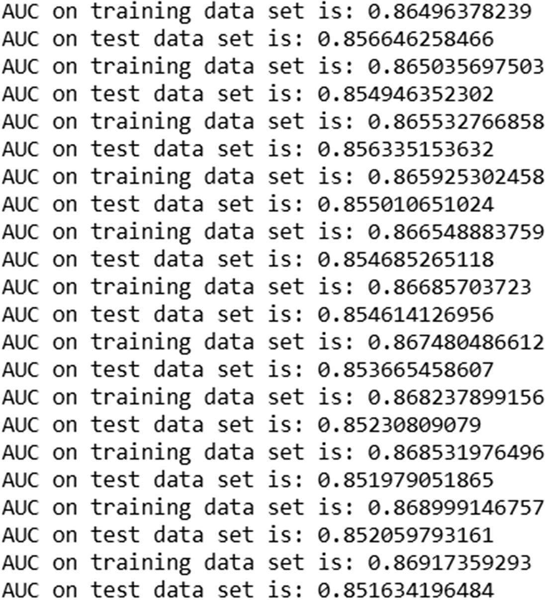
Note that the AUC of train dataset keeps on increasing with more trees. But the AUC of the test dataset decreases after a certain iteration.

Shrinkage

GBM is based on decision tree. So, just like Random Forest algorithm, the accuracy of GBM depends on the depth of trees considered, number of trees built and the minimum number of observations in a terminal node. Shrinkage is an additional parameter in GBM. Let’s see what happens to the output of the train and test dataset AUC if we change the learning rate/shrinkage. We’ll initialize the learning rate to be equal to 0.05 and run more trees:

from sklearn.model_selection import train_test_split

# creating independent variables

X = data.drop('SeriousDlqin2yrs',axis=1)

# creating dependent variables

y = data['SeriousDlqin2yrs']

# creating train and test datasets

X_train, X_test, y_train, y_test = train_test_split(X, y, test_size=0.30, random_state=42)

from sklearn.tree import DecisionTreeClassifier

depth_tree = DecisionTreeClassifier(criterion = "gini",max_depth=4, min_samples_leaf=10)

depth_tree.fit(X_train, y_train)

#Get the predictions on top of train and test datasets

dt_pred = depth_tree.predict_proba(X_train)

X_train['prediction']=dt_pred[:,1]

X_test['prediction']=depth_tree.predict_proba(X_test)[:,1]

from sklearn.tree import DecisionTreeRegressor

import numpy as np

from sklearn.metrics import roc_auc_score

depth_tree2 = DecisionTreeRegressor(criterion = "mse",max_depth=4, min_samples_leaf=10)

learning_rate = 0.05

for i in range(20):

# Calculate residual

train_errorn=y_train-X_train['prediction']

# remove prediction variable that got appended to independent variable earlier

X_train2=X_train.drop(['prediction'],axis=1)

X_test2=X_test.drop(['prediction'],axis=1)

# Build a decision tree to predict the residuals using independent variables

dt2=depth_tree2.fit(X_train2, train_errorn)

# predict the residual

dt_pred_train_errorn = dt2.predict(X_train2)

# update the predictions based on predicted residuals

X_train['prediction']=(X_train['prediction']+dt_pred_train_errorn*learning_rate)

# Calculate AUC

train_auc=roc_auc_score(y_train,X_train['prediction'])

print("AUC on training data set is: "+str(train_auc))

# update the predictions based on predicted residuals for test dataset

dt_pred_test_errorn = dt2.predict(X_test2)

X_test['prediction']=(X_test['prediction']+dt_pred_test_errorn*learning_rate)

# Calculate AUC

test_auc=roc_auc_score(y_test,X_test['prediction'])

print("AUC on test data set is: "+str(test_auc))

The output of the preceding code is:

Here is the output of the first few trees:

../images/463052_1_En_6_Chapter/463052_1_En_6_Figc_HTML.jpg

And here is the output of the last few trees:

../images/463052_1_En_6_Chapter/463052_1_En_6_Figd_HTML.jpg

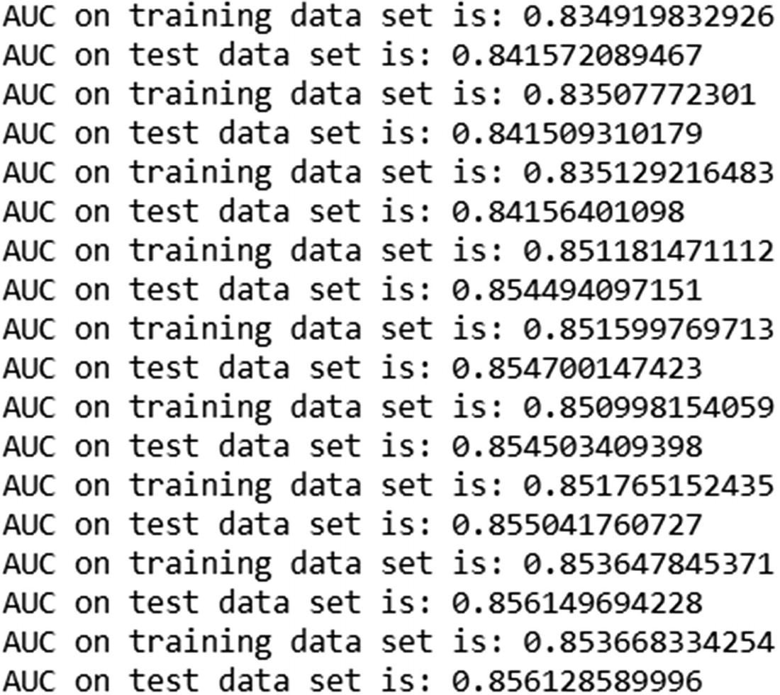
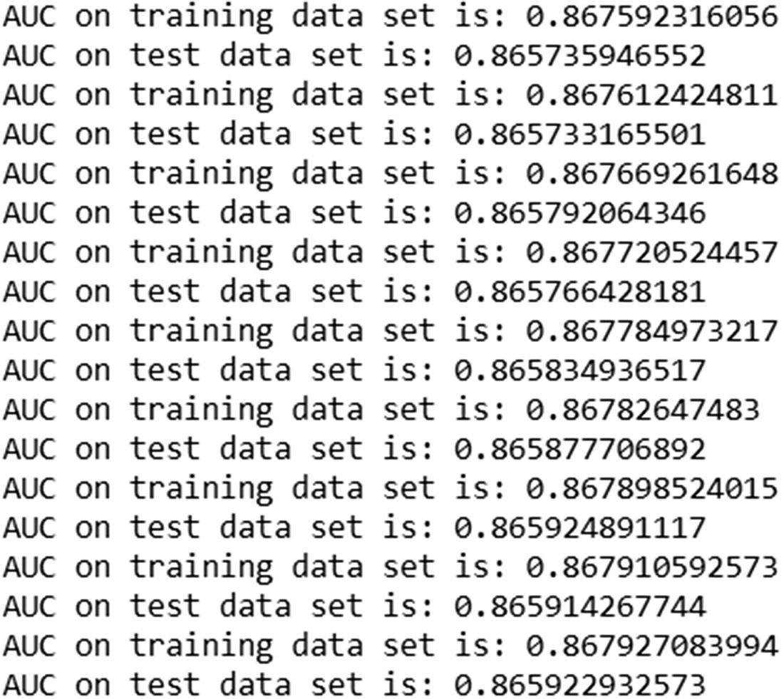
Unlike in the previous case, where learning_rate = 1, lower learning_rate resulted in the test dataset AUC increasing consistently along with the training dataset AUC.

AdaBoost

Before proceeding to the other methods of boosting, I want to draw a parallel from what we’ve seen in previous chapters. While calculating the error metric for logistic regression, we could have gone with the traditional squared error. But we moved to the entropy error, because it penalizes more for high amount of error.

In a similar manner, residual calculation can vary by the type of dependent variable. For a continuous dependent variable, residual calculation can be Gaussian ((actual – prediction) of dependent variable), whereas for a discrete variable, residual calculation could be different.

Theory of AdaBoost

AdaBoost is short for adaptive boosting. Here is the high-level algorithm:

1.
Build a weak learner (decision tree technique in this case) using only a few independent variables.
1. a.
  Note that while building the first weak learner, the weightage associated with each observation is the same.
2.
Identify the observations that are classified incorrectly based on the weak learner.
3.
Update the weights of the observations in such a way that the misclassifications in the previous weak learner are given more weightage and the correct classifications in the previous weak learner are given less weightage.
4.
Assign a weightage for each weak learner based on the accuracy of its predictions.
5.
The final prediction will be based on the weighted average prediction of multiple weak learners.

Adaptive potentially refers to the updating of weights of observations, depending on whether the previous classification was correct or incorrect. Boosting potentially refers to assigning the weightages to each weak learner.

Working Details of AdaBoost

Let’s look at an example of AdaBoost:

1.
Build a weak learner.
Let’s say the dataset is the first two columns in the following table (available as “adaboost.xlsx” in github):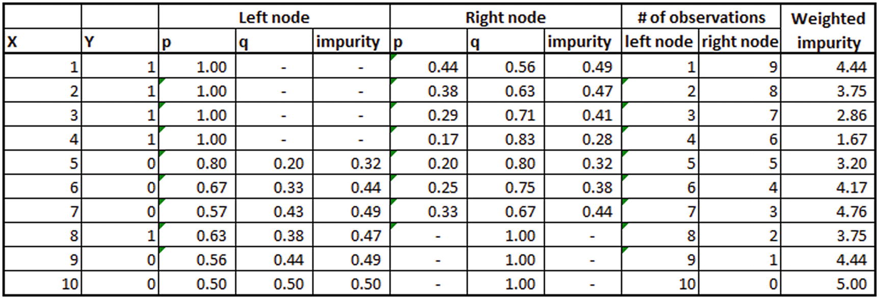
Once we have the dataset, we build a weak learner (decision tree) according to the steps laid out to the right in the preceding table. From the table we can see that X <= 4 is the optimal splitting criterion for this first decision tree.
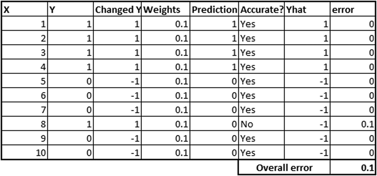
2.
Calculate the error metric (the reason for having “Changed Y” and “Yhat” as new columns in the below table will be explained after step 4):
The formulae used to obtain the preceding table are as follows:
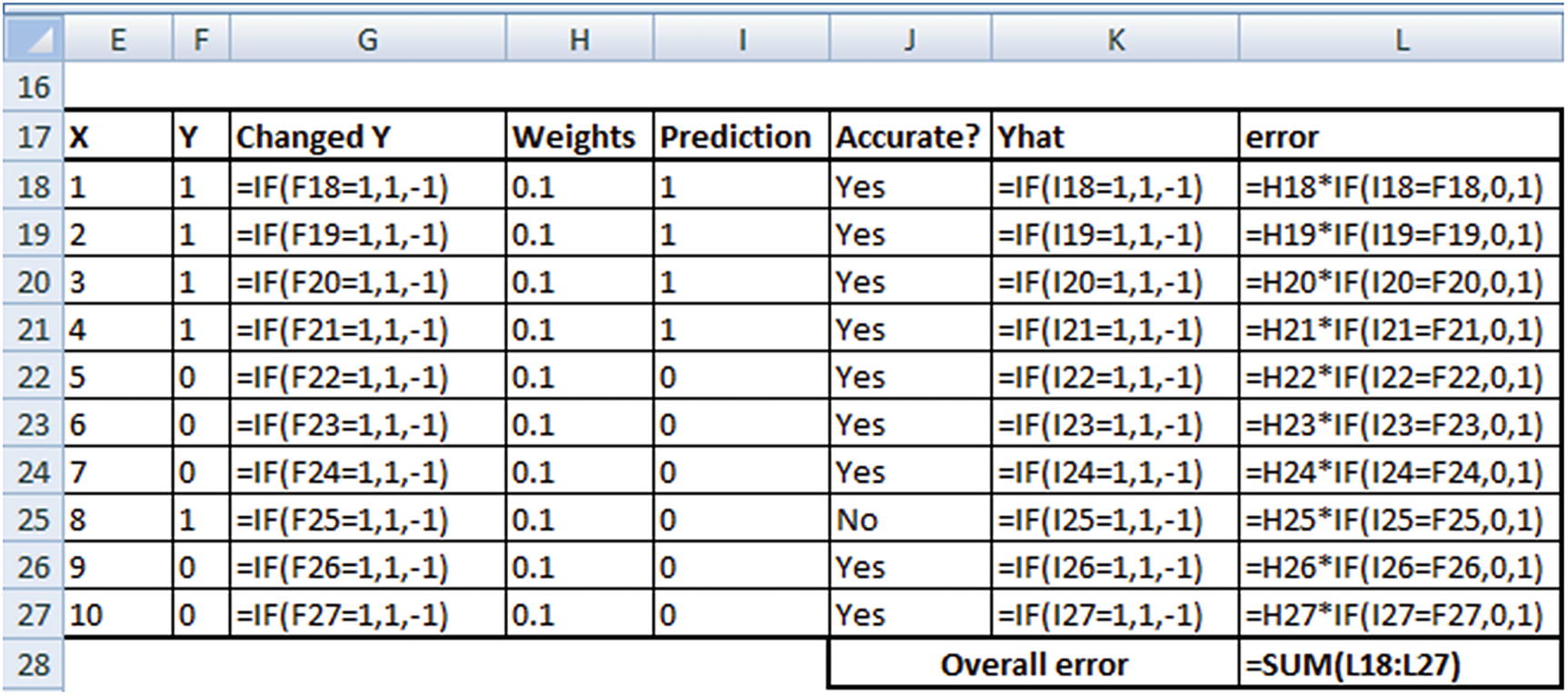
3.
Calculate the weightage that should be associated with the first weak learner:
0.5 × log((1 – error)/error) = 0.5 × log(0.9 / 0.1) = 0.5 × log(9) = 0.477
4.
Update the weights associated with each observation in such a way that the previous weak learner’s misclassifications have high weight and the correct classifications have low weight (essentially, we are tuning the weights associated with each observation in such a way that, in the new iteration, we try and make sure that the misclassifications are predicted more accurately):
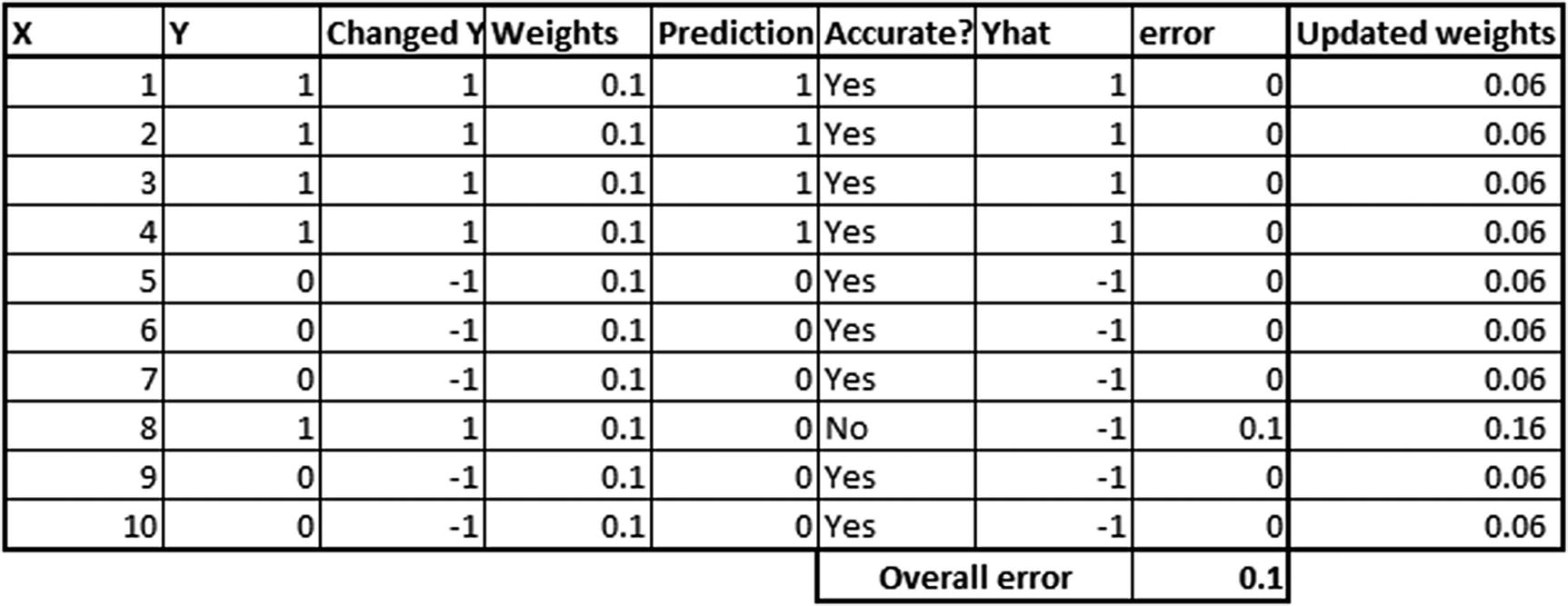Note that the updated weights are calculated by the following formula:
${original\kern0.34em weight}^{\ast}\kern0.125em {e}^{\left(- weightage\ oflearner\ast yhat\ast changedy\right)}$
That formula should explain the need for changing the discrete values of y from {0,1} to {–1,1}. By changing 0 to –1, we are in a position to perform the multiplication better. Also note that in the preceding formula, weightage associated with the learner in general would more often than not be positive.
When yhat and changed_y are the same, the exponential part of formula would be a lower number (as the – weightage of learner × yhat × changed_y part of the formula would be negative, and an exponential of a negative is a small number).
When yhat and changed_y are different values, that’s when the exponential would be a bigger number, and hence the updated weight would be more than the original weight.
5.
We observe that the updated weights we obtained earlier do not sum up to 1. We update each weight in such a way that the sum of weights of all observations is equal to 1. Note that, the moment weights are introduced, we can consider this as a regression exercise.
Now that the weight for each observation is updated, we repeat the preceding steps until the weight of the misclassified observations increases so much that it is now correctly classified: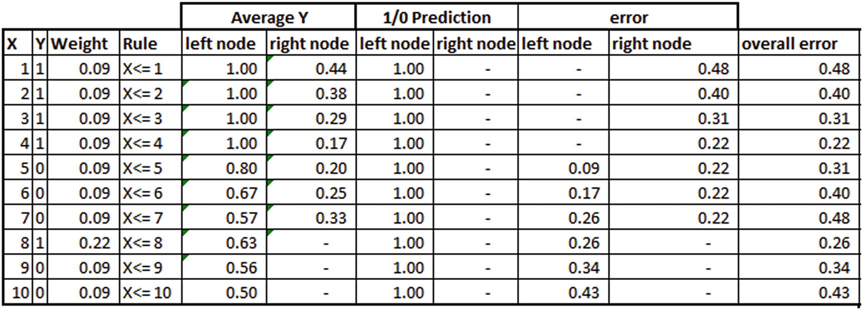
Note that the weights in the third column in the preceding table are updated based on the formula we derived earlier post normalization (ensuring that the sum of weights is 1).
You should be able to see that the weight associated with misclassification (the eighth observation with the independent variable value of 8) is more than any other observation.
Note that although everything is similar to a typical decision tree till the prediction columns, error calculation gives emphasis to weights of observations. error in the left node is the summation of the weight of each observation that was misclassified in the left node and similarly for the right node.
overall error is the summation of error across both nodes (error in left node + error in right node).
In this instance, overall error is still the least at the fourth observation.
The updated weights based on the previous step are as follows: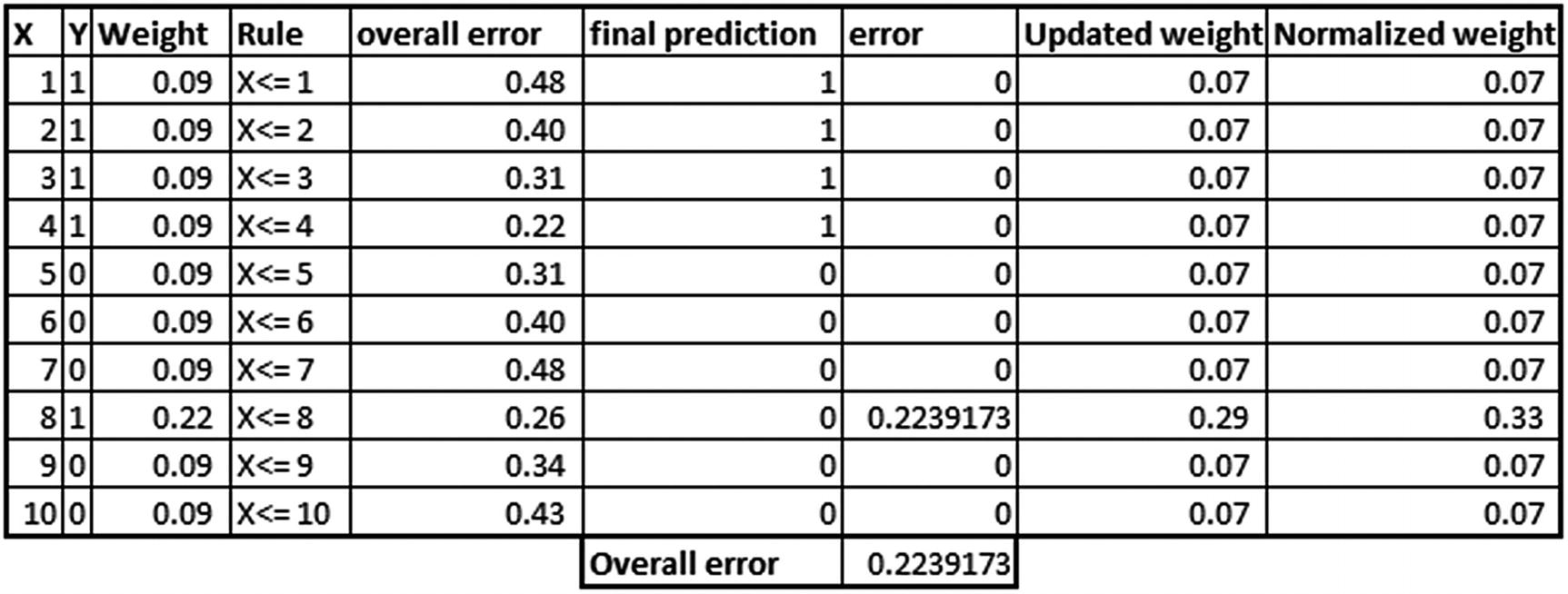
Continue the process one more time:
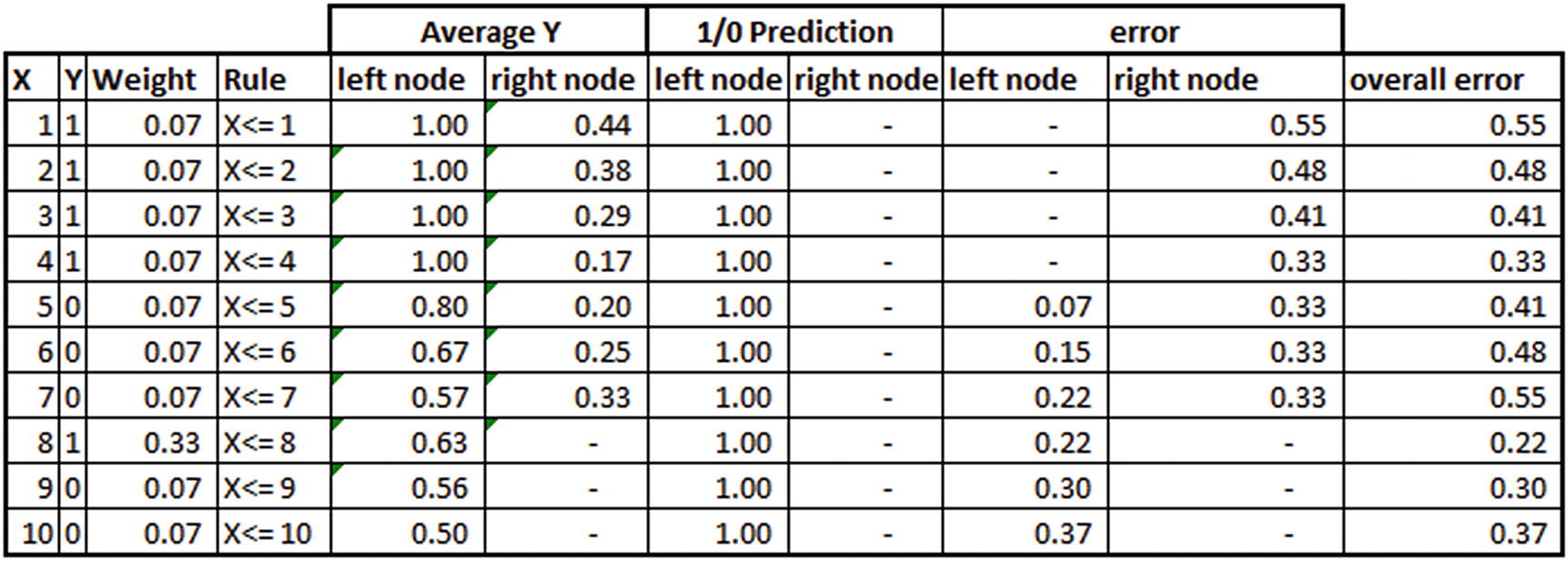
From the preceding table, note that overall error in this iteration is minimum at X <= 8, as the weight associated with the eighth observation is a lot more than other observations, and hence overall error came up as the least at the eighth observation this time. However, note that the weightage associated with the preceding tree would be low, because the accuracy of that tree is low when compared to the previous two trees.
6.
Once all the predictions are made, the final prediction for an observation is calculated as the summation of the weightage associated with each weak learner multiplied by the probability output for each observation.

Additional Functionality for GBM

In the previous section, we saw how to hand construct GBM. In this section, we will look at other parameters that can be built in:

Row sampling: In random forest, we saw that sampling a random selection of rows results in a more generalized and better model. In GBM, too, we can potentially sample rows to improve the model performance further.
Column sampling: Similar to row sampling, some amount of overfitting can be avoided by sampling columns for each decision tree.

Both random forest and GBM techniques are based on decision tree. However, a random forest can be thought of as building multiple trees in parallel, where in the end we take the average of all the multiple trees as the final prediction. In a GBM, we build multiple trees, but in sequence, where each tree tries to predict the residual of its previous tree.

Implementing GBM in Python

GBM can be implemented in Python using the scikit-learn library as follows (code is available as “GBM.ipynb” in github):

from sklearn import ensemble

gb_tree = ensemble.GradientBoostingClassifier(loss='deviance',learning_rate=0.05,n_estimators=100,min_samples_leaf=10,max_depth=13,max_features=2,subsample=0.7,random_state=10)

gb_tree.fit(X_train, y_train)

Note that the key input parameters are a loss function (whether it is a normal residual approach or an AdaBoost-based approach), learning rate, number of trees, depth of each tree, column sampling, and row sampling.

Once a GBM is built, the predictions can be made as follows:

from sklearn.metrics import roc_auc_score

gb_pred=gb_tree.predict_proba(X_test)

roc_auc_score(y_test, gb_pred[:,1])

Implementing GBM in R

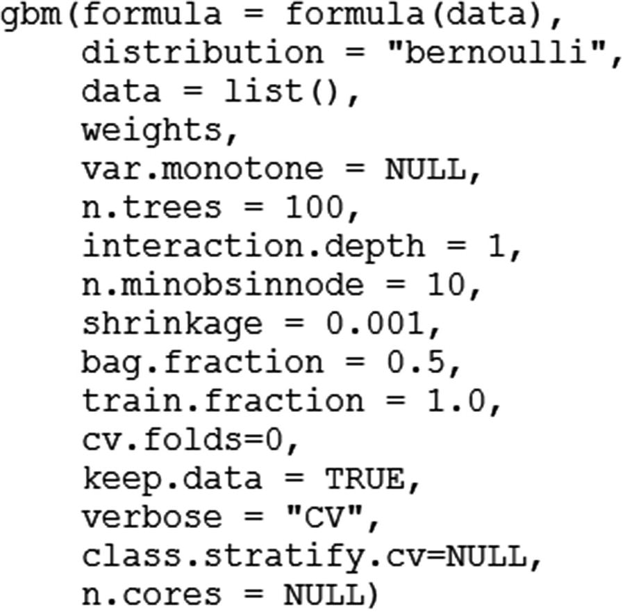
GBM in R has similar parameters to GBM in Python. GBM can be implemented as follows:

../images/463052_1_En_6_Chapter/463052_1_En_6_Figl_HTML.jpg

In that formula, we specify the dependent and independent variables in the following fashion: dependent_variable ~ the set of independent variables to be used.

The distribution specifies whether it is a Gaussian, Bernoulli, or AdaBoost algorithm.

n. trees specifies the number of trees to be built.
interaction.depth is the max_depth of the trees.
n.minobsinnode is the minimum number of observations in a node.
shrinkage is the learning rate.
bag.fraction is the fraction of the training set observations randomly selected to propose the next tree in the expansion.
GBM algorithm in R is run as follows:

library(gbm)

gb=gbm(SeriousDlqin2yrs~.,data=train,n.trees=10,interaction.depth=5,shrinkage=0.05)

The predictions can be made as follows:

pred=predict(gb,test,n.trees=10,type="response")

Summary

In this chapter, you learnt the following:

GBM is a decision tree–based algorithm that tries to predict the residual of the previous decision tree in a given decision tree.
Shrinkage and depth are some of the more important parameters that need to be tuned within GBM.
The difference between gradient boosting and adaptive boosting.
How tuning the learning rate parameter improves prediction accuracy in GBM.

Previous Chapter

5. Random Forest

Next Chapter

7. Artificial Neural Network

Table of Contents for Pro Machine Learning Algorithms : A Hands-On Approach to Implementing Algorithms in Python and R

6. Gradient Boosting Machine

Gradient Boosting Machine

Working details of GBM

Shrinkage

AdaBoost

Theory of AdaBoost

Working Details of AdaBoost

Additional Functionality for GBM

Implementing GBM in Python

Implementing GBM in R

Summary

Table of Contents for
Pro Machine Learning Algorithms : A Hands-On Approach to Implementing Algorithms in Python and R