V Kishore AyyadevaraPro Machine Learning Algorithms https://doi.org/10.1007/978-1-4842-3564-5_2

2. Linear Regression

V Kishore Ayyadevara¹

(1)

Hyderabad, Andhra Pradesh, India

In order to understand linear regression, let’s parse it:

Linear: Arranged in or extending along a straight or nearly straight line, as in “linear movement.”
Regression: A technique for determining the statistical relationship between two or more variables where a change in one variable is caused by a change in another variable.

Combining those, we can define linear regression as a relationship between two variables where an increase in one variable impacts another variable to increase or decrease proportionately (that is, linearly).

In this chapter, we will learn the following:

How linear regression works
Common pitfalls to avoid while building linear regression
How to build linear regression in Excel, Python, and R

Introducing Linear Regression

Linear regression helps in interpolating the value of an unknown variable (a continuous variable) based on a known value. An application of it could be, “What is the demand for a product as the price of the product is varied?” In this application, we would have to look at the demand based on historical prices and make an estimate of demand given a new price point.

Given that we are looking at history in order to estimate a new price point, it becomes a regression problem. The fact that price and demand are linearly related to each other (the higher the price, the lower the demand and vice versa) makes it a linear regression problem.

Variables: Dependent and Independent

A dependent variable is the value that we are predicting for, and an independent variable is the variable that we are using to predict a dependent variable.

For example, temperature is directly proportional to the number of ice creams purchased. As temperature increases, the number of ice creams purchased would also increase. Here temperature is the independent variable, and based on it the number of ice creams purchased (the dependent variable) is predicted.

Correlation

From the preceding example, we may notice that ice cream purchases are directly correlated (that is, they move in the same or opposite direction of the independent variable, temperature) with temperature. In this example, the correlation is positive: as temperature increases, ice cream sales increase. In other cases, correlation could be negative: for example, sales of an item might increase as the price of the item is decreased.

Causation

Let’s flip the scenario that ice cream sales increase as temperature increases (high + ve correlation). The flip would be that temperature increases as ice cream sales increase (high + ve correlation, too).

However, intuitively we can say with confidence that temperature is not controlled by ice cream sales, although the reverse is true. This brings up the concept of causation —that is, which event influences another event. Temperature influences ice cream sales—but not vice versa.

Simple vs. Multivariate Linear Regression

We’ve discussed the relationship between two variables (dependent and independent). However, a dependent variable is not influenced by just one variable but by a multitude of variables. For example, ice cream sales are influenced by temperature, but they are also influenced by the price at which ice cream is being sold, along with other factors such as location , ice cream brand, and so on.

In the case of multivariate linear regression, some of the variables will be positively correlated with the dependent variable and some will be negatively correlated with it.

Formalizing Simple Linear Regression

Now that we have the basic terms in place, let’s dive into the details of linear regression. A simple linear regression is represented as:

$Y=a+{b}^{\ast }X$

Y is the dependent variable that we are predicting for.
X is the independent variable.
a is the bias term.
b is the slope of the variable (the weight assigned to the independent variable).

Y and X, the dependent and independent variables should be clear enough now. Let’s get introduced to the bias and weight terms (a and b in the preceding equation).

The Bias Term

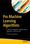
Let’s look at the bias term through an example: estimating the weight of a baby by the baby’s age in months. We’ll assume that the weight of a baby is solely dependent on how many months old the baby is. The baby is 3 kg when born and its weight increases at a constant rate of 0.75 kg every month .

At the end of year, the chart of baby weight looks like Figure 2-1.

../images/463052_1_En_2_Chapter/463052_1_En_2_Fig1_HTML.jpg — Figure 2-1
Baby weight over time in months

In Figure 2-1, the baby’s weight starts at 3 (a, the bias) and increases linearly by 0.75 (b, the slope) every month. Note that, a bias term is the value of the dependent variable when all the independent variables are 0.

The Slope

The slope of a line is the difference between the x and y coordinates at both extremes of the line upon the length of line. In the preceding example, the value of slope (b) is as follows:

(Difference between y coordinates at both extremes) / (Difference between x coordinates at both extremes)

$b=\frac{12-3\ }{\left(12-0\right)}=9/12=0.75$

Solving a Simple Linear Regression

We’ve seen a simple example of how the output of a simple linear regression might look (solving for bias and slope). In this section, we’ll take the first steps towards coming up with a more generalized way to generate a regression line. The dataset provided is as follows:

Age in months	Weight in kg
0	3
1	3.75
2	4.5
3	5.25
4	6
5	6.75
6	7.5
7	8.25
8	9
9	9.75
10	10.5
11	11.25
12	12

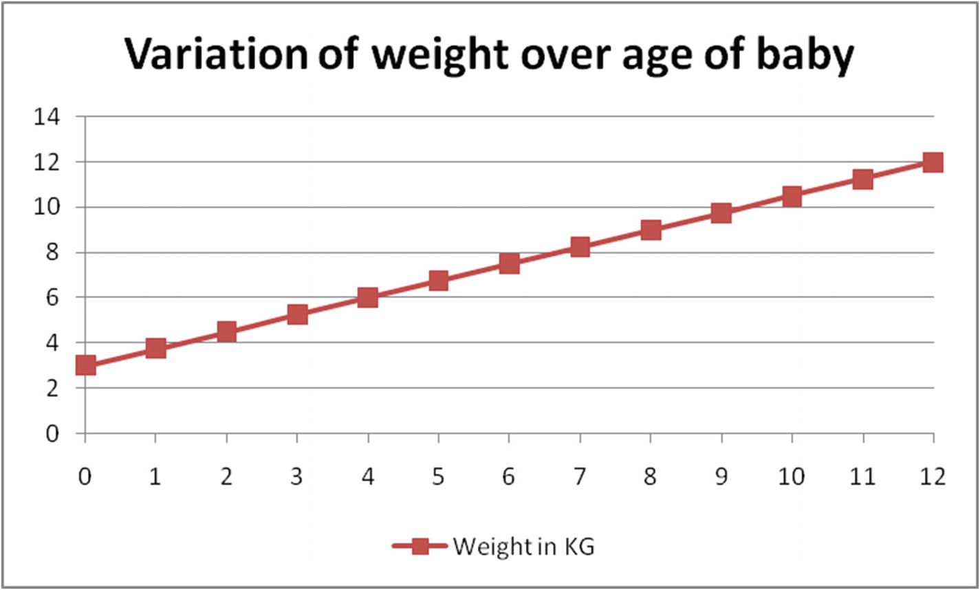
A visualization of the data is shown in Figure 2-2.

../images/463052_1_En_2_Chapter/463052_1_En_2_Fig2_HTML.jpg — Figure 2-2
Visualizing baby weight

In Figure 2-2, the x-axis is the baby’s age in months, and the y-axis is the weight of the baby in a given month. For example, the weight of the baby in the first month is 3.75 kg.

Let’s solve the problem from first principles. We’ll assume that the dataset has only 2 data points, not 13—but, just the first 2 data points. The dataset would look like this:

Age in months	Weight in kg
0	3
1	3.75

Given that we are estimating the weight of the baby based on its age, the linear regression can be built as follows:

$3=a+{b}^{\ast }(0)$

$3.75=a+{b}^{\ast }(1)$

Solving that, we see that a = 3 and b = 0.75.

Let’s apply the values of a and b on the remaining 11 data points above. The result would look like this:

Age in months	Weight In kg	Estimate of weight
0	3	3
1	3.75	3.75
2	4.5	4.5
3	5.25	5.25
4	6	6
5	6.75	6.75
6	7.5	7.5
7	8.25	8.25
8	9	9
9	9.75	9.75
10	10.5	10.5
11	11.25	11.25
12	12	12
		Overall squared error

As you can see, the problem can be solved with minimal error rate by solving the first two data points only. However, this would likely not be the case in practice because most real data is not as clean as is presented in the table.

More General Way of Solving a Simple Linear Regression

In the preceding scenario, we saw that the coefficients are obtained by using just two data points from the total dataset—that is, we have not considered a majority of the observations in coming up with optimal a and b. To avoid leaving out most of the data points while building the equation, we can modify the objective as minimizing the overall squared error (ordinary least squares) across all the data points.

Minimizing the Overall Sum of Squared Error

Overall squared error is defined as the sum of the squared difference between actual and predicted values of all the observations. The reason we consider squared error value and not the actual error value is that we do not want positive error in some data points offsetting for negative error in other data points. For example, an error of +5 in three data points offsets an error of –5 in three other data points, resulting in an overall error of 0 among the six data points combined. Squared error converts the –5 error of the latter three data points into a positive number, so that the overall squared error then becomes 6 × 5² = 150.

This brings up a question: why should we minimize overall squared error? The principle is as follows:

1.
Overall error is minimized if each individual data point is predicted correctly.
2.
In general, overprediction by 5% is equally as bad as underprediction by 5%, hence we consider the squared error.

Let’s formulate the problem:

Age in months	Weight in kg	Formula	Estimate of weight when a = 3 and b = 0.75
0	3	3 = a + b × (0)	3
1	3.75	3.75 = a + b × (1)	3.75
2	4.5	4.5 = a + b × (2)	4.5
3	5.25	5.25 = a + b × (3)	5.25
4	6	6 = a + b × (4)	6
5	6.75	6.75 = a + b × (5)	6.75
6	7.5	7.5 = a + b × (6)	7.5
7	8.25	8.25 = a + b × (7)	8.25
8	9	9 = a + b × (8)	9
9	9.75	9.75 = a + b × (9)	9.75
10	10.5	10.5 = a + b × (10)	10.5
11	11.25	11.25 = a + b × (11)	11.25
12	12	12 = a + b × (12)	12
			Overall squared error

Linear regression equation is represented in the Formula column in the preceding table.

Once the dataset (the first two columns) are converted into a formula (column 3), linear regression is a process of solving for the values of a and b in the formula column so that the overall squared error of estimate (the sum of squared error of all data points) is minimized.

Solving the Formula

The process of solving the formula is as simple as iterating over multiple combinations of a and b values so that the overall error is minimized as much as possible. Note that the final combination of optimal a and b value is obtained by using a technique called gradient descent , which is explored in Chapter 7.

Working Details of Simple Linear Regression

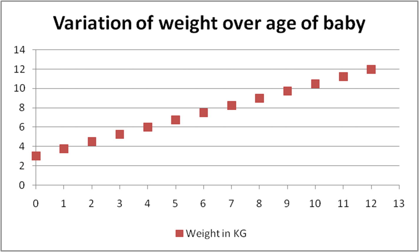
Solving for a and b can be understood as a goal seek problem in Excel, where Excel is helping identify the values of a and b that minimize the overall value.

To see how this works, look at the following dataset (available as “linear regression 101.xlsx” in github):

../images/463052_1_En_2_Chapter/463052_1_En_2_Figa_HTML.jpg

You should understand the following by checking the below in dataset:

1.
How cells H3 and H4 are related to column D (estimate of weight)
2.
The formula of column E
3.
Cell E15, the sum of squared error for each data point
4.
To obtain the optimal values of a and b (in cells H3 and H4)—go to Solver in Excel and add the following constraints:
1. a.
  Minimize the value in cell E15
2. b.
  By changing cells H3 and H4

Complicating Simple Linear Regression a Little

In the preceding example, we started with a scenario where the values fit perfectly: a = 3 and b = 0.75.

The reason for zero error rate is that we defined the scenario first and then defined the approach—that is, a baby is 3 kg at birth and the weight increases by 0.75 kg every month. However, in practice the scenario is different: “Every baby is different.”

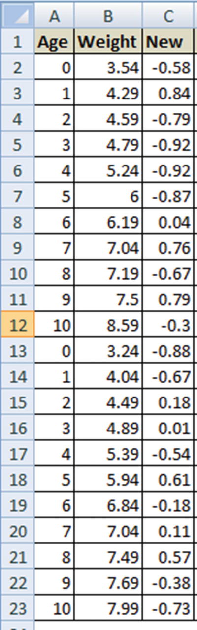
Let’s visualize this new scenario through a dataset (available as “Baby age to weight relation.xlsx” in github). Here, we have the age and weight measurement of two different babies.

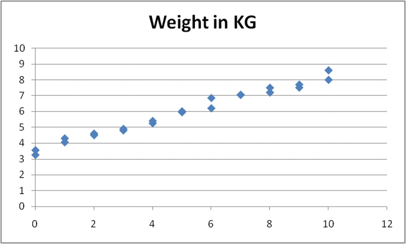
The plot of age-to-weight relationship now looks like Figure 2-3.

../images/463052_1_En_2_Chapter/463052_1_En_2_Fig3_HTML.jpg — Figure 2-3
Age-to-weight reltionship

The value of weight increases as age increases, but not in the exact trend of starting at 3 kg and increasing by 0.75 kg every month, as seen in the simplest example.

To solve for this, we go through the same rigor we did earlier:

1.
Initialize with arbitrary values of a and b (for example, each equals 1).
2.
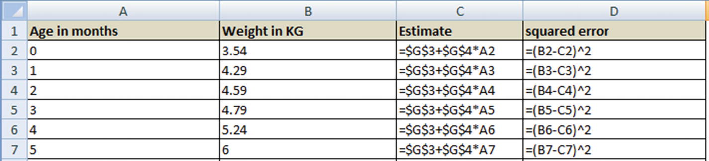
Make a new column for the forecast with the value of a + b × X – column C.
3.
Make a new column for squared error, column D.
4.
Calculate overall error in cell G7.
5.
Invoke the Solver to minimize cell G7 by changing cells a and b —that is, G3 and G4.

../images/463052_1_En_2_Chapter/463052_1_En_2_Figc_HTML.jpg

The cell connections in the preceding scenario are as follows:

../images/463052_1_En_2_Chapter/463052_1_En_2_Figd_HTML.jpg

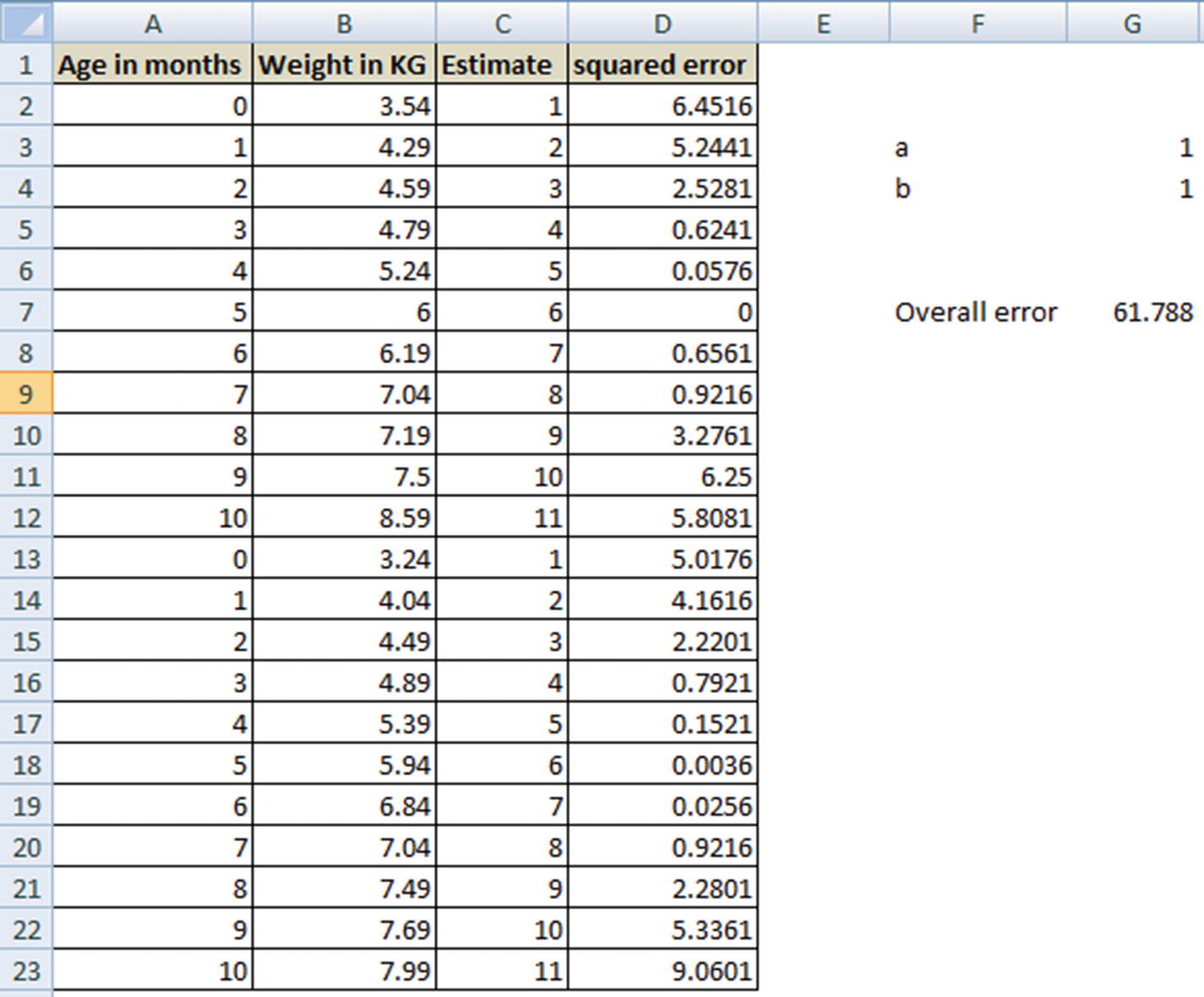
The cell values of G3 and G4 that minimize the overall error are the optimal values of a and b.

Arriving at Optimal Coefficient Values

Optimal values of coefficients are arrived at using a technique called gradient descent. Chapter 7 contains a detailed discussion of how gradient descent works, but for now, let’s begin to understand gradient descent using the following steps:

1.
Initialize the value of coefficients (a and b) randomly.
2.
Calculate the cost function—that is, the sum of squared error across all the data points in the training dataset.
3.
Change the value of coefficients slightly, say, +1% of its value.
4.
Check whether, by changing the value of coefficients slightly, overall squared error decreases or increases.
5.
If overall squared error decreases by changing the value of coefficient by +1%, then proceed further, else reduce the coefficient by 1%.
6.
Repeat steps 2–4 until overall squared error is the least.

Introducing Root Mean Squared Error

So far, we have seen that the overall error is the sum of the square of difference between forecasted and actual values for each data point. Note that, in general, as the number of data points increase, the overall squared error increases.

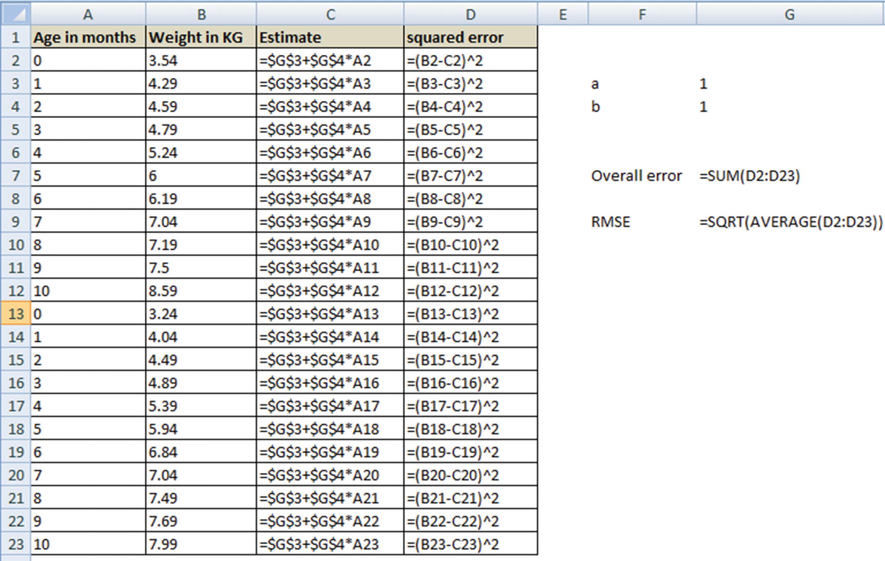
In order to normalize for the number of observations in data—that is, having a meaningful error measure, we would consider the square root of mean of error (as we have squared the difference while calculating error) . Root mean squared error (RMSE) is calculated as follows (in cell G9):

../images/463052_1_En_2_Chapter/463052_1_En_2_Fige_HTML.jpg

Note that in the preceding dataset, we would have to solve for the optimal values of a and b (cells G3 and G4) that minimize the overall error .

Running a Simple Linear Regression in R

To understand the implementation details of the material covered in the preceding sections, we’ll run the linear regression in R (available as “simple linear regression.R” in github).

# import file

data=read.csv("D:/Pro ML book/linear_reg_example.csv")

# Build model

lm=glm(Weight~Age,data=data)

# summarize model

summary(lm)

The function lm stands for linear model, and the general syntax is as follows:

lm(y~x,data=data)

where y is the dependent variable, x is the independent variable, and data is the dataset.

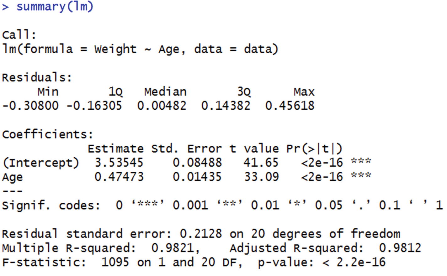
summary(lm) gives a summary of the model along with the variables that came in significant, along with some automated tests. Let’s parse them one at a time:

../images/463052_1_En_2_Chapter/463052_1_En_2_Figf_HTML.jpg

Residuals

Residual is nothing but the error value (the difference between actual and forecasted value). The summary function automatically gives us the distribution of residuals. For example, consider the residuals of the model on the dataset we trained.

Distribution of residuals using the model is calculated as follows:

#Extracting prediction

data$prediction=predict(lm,data)

# Extracting residuals

data$residual = data$Weight - data$prediction

# summarizing the residuals

summary(data$residual)

In the preceding code snippet, the predict function takes the model to implement and the dataset to work on as inputs and produces the predictions as output.

Note

The output of the summary function is the various quartile values in the residual column.

Coefficients

The coefficients section of the output gives a summary version of the intercept and bias that got derived. (Intercept) is the bias term (a), and Age is the independent variable:

Estimate is the value of a and b each.
Std error gives us a sense of variation in the values of a and b if we draw random samples from the total population. Lower the ratio of standard error to intercept, more stable is the model.

Let’s look at a way in which we can visualize/calculate the standard error values. The following steps extract the standard error value:

1.
Randomly sample 50% of the total dataset.
2.
Fit a lm model on the sampled data.
3.
Extract the coefficient of the independent variable for the model fitted on sampled data.
4.
Repeat the whole process over 100 iterations.

In code, the preceding would translate as follows:

# Initialize an object that stores the various coefficient values

samp_coef=c()

# Repeat the experiment 100 times

for(i in 1:100){

# sample 50% of total data

samp=sample(nrow(data),0.5*nrow(data))

data2=data[samp,]

# fit a model on the sampled data

lm=lm(Weight~Age,data=data2)

# extract the coefficient of independent variable and store it

samp_coef=c(samp_coef,lm$coefficients['Age'])

}

sd(samp_coef)

Note that the lower the standard deviation, the closer the coefficient values of sample data are to the original data. This indicates that the coefficient values are stable regardless of the sample chosen.

t-value is the coefficient divided by the standard error. The higher the t-value, the better the model stability.

Consider the following example:

../images/463052_1_En_2_Chapter/463052_1_En_2_Figg_HTML.jpg

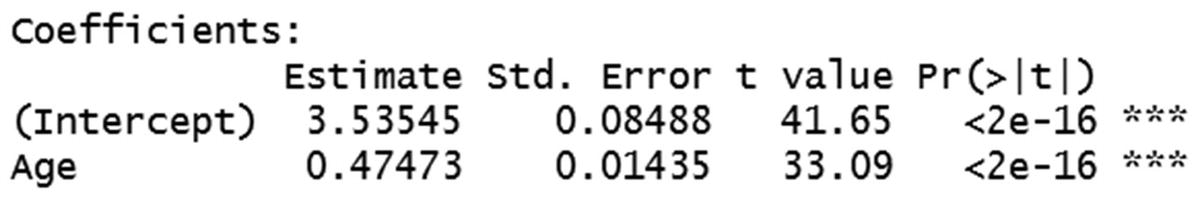
The t-value corresponding to the variable Age would equal 0.47473/0.01435. (Pr>|t|) gives us the p-value corresponding to t-value. The lower the p-value, the better the model is. Let us look at the way in which we can derive p-value from t-value. A lookup for t-value to p-value is available in the link here: http://www.socscistatistics.com/pvalues/tdistribution.aspx

In our case, for the Age variable, t-value is 33.09.

Degrees of freedom = Number of rows in dataset – (Number of independent variables in model + 1) = 22 – (1 +1) = 20

Note that the +1 in the preceding formula comes from including the intercept term.

We would check for a two-tailed hypothesis and input the value of t and the degrees of freedom into the lookup table, and the output would be the corresponding p-value.

As a rule of thumb, if a variable has a p-value < 0.05, it is accepted as a significant variable in predicting the dependent variable. Let’s look at the reason why.

If the p-value is high, it’s because the corresponding t-value is low, and that’s because the standard error is high when compared to the estimate, which ultimately signifies that samples drawn randomly from the population do not have similar coefficients.

In practice, we typically look at p-value as one of the guiding metrics in deciding whether to include an independent variable in a model or not.

SSE of Residuals (Residual Deviance)

The sum of squared error of residuals is calculated as follows:

# SSE of residuals

data$prediction = predict(lm,data)

sum((data$prediction-data$Weight)^2)

Residual deviance signifies the amount of deviance that one can expect after building the model. Ideally the residual deviance should be compared with null deviance—that is, how much the deviance has decreased because of building a model.

Null Deviance

A null deviance is the deviance expected when no independent variables are used in building the model .

The best guess of prediction, when there are no independent variables, is the average of the dependent variable itself. For example, if we say that, on average, there are $1,000 in sales per day, the best guess someone can make about a future sales value (when no other information is provided) is $1,000.

Thus, null deviance can be calculated as follows:

#Null deviance

data$prediction = mean(data$Weight)

sum((data$prediction-data$Weight)^2)

Note that, the prediction is just the mean of the dependent variable while calculating the null deviance .

R Squared

R squared is a measure of correlation between forecasted and actual values. It is calculated as follows:

1.
Find the correlation between actual dependent variable and the forecasted dependent variable.
2.
Square the correlation obtained in step 1—that is the R squared value.

R squared can also be calculated like this:

$1-\left( Residual\ deviance/ Null\ deviance\right)$

Null deviance—the deviance when we don’t use any independent variable (but the bias/constant) in predicting the dependent variable—is calculated as follows:

$null\ deviance=\sum {\left(Y\hbox{--} \widehat{Y}\right)}^2$

where is the dependent variable and $\widehat{Y}$ is the average of the dependent variable.

Residual deviance is the actual deviance when we use the independent variables to predict the dependent variable. It’s calculated as follows:

$residual\ deviance=\sum {\left(Y\hbox{--} \overline{y}\right)}^2$

where Y is the actual dependent variable and $\overline{y}$ is the predicted value of the dependent variable.

Essentially, R squared is high when residual deviance is much lower when compared to the null deviance.

F-statistic

F-statistic gives us a similar metric to R-squared. The way in which the F-statistic is calculated is as follows:

$F=\left(\frac{\frac{SSE(N)- SSE(R)}{d{f}_N-d{f}_R}}{\frac{SSE(R)}{d{f}_R}}\right)$

where SSE(N) is the null deviance, SSE(R) is the residual deviance, df _N is the degrees of freedom of null deviance, and df _R is the degrees of freedom of residual deviance. The higher the F-statistic , the better the model. The higher the reduction in deviance from null deviance to residual deviance, the higher the predictability of using the independent variables in the model will be.

Running a Simple Linear Regression in Python

A linear regression can be run in Python using the following code (available as “Linear regression Python code.ipynb” in github):

# import relevant packages

# pandas package is used to import data

# statsmodels is used to invoke the functions that help in lm

import pandas as pd

import statsmodels.formula.api as smf

# import dataset

data = pd.read_csv('D:/Pro ML book/Linear regression/linear_reg_example.csv')

# run least squares regression

est = smf.ols(formula='Weight~Age',data=data)

est2=est.fit()

print(est2.summary())

The output of the preceding codes looks like this:

../images/463052_1_En_2_Chapter/463052_1_En_2_Figh_HTML.jpg

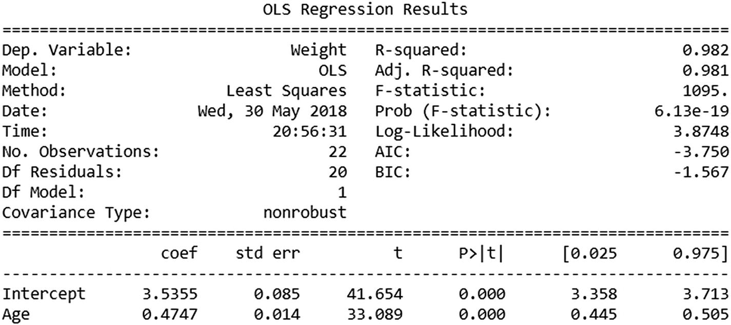
Note that the coefficients section outputs of R and Python are very similar. However, this package has given us more metrics to study the level of prediction by default. We will look into those in more detail in a later section.

Common Pitfalls of Simple Linear Regression

The simple examples so far are to illustrate the basic workings of linear regression. Let’s consider scenarios where it fails:

When the dependent and independent variables are not linearly related with each other throughout: As the age of a baby increases, the weight increases, but the increase plateaus at a certain stage, after which the two values are not linearly dependent any more. Another example here would be the relation between age and height of an individual.
When there is an outlier among the values within independent variables: Say there is an extreme value (a manual entry error) within a baby’s age. Because our objective is to minimize the overall error while arriving at the a and b values of a simple linear regression, an extreme value in the independent variables can influence the parameters by quite a bit. You can see this work by changing the value of any age value and calculating the values of a and b that minimize the overall error. In this case, you would note that even though the overall error is low for the given values of a and b, it results in high error for a majority of other data points.

In order to avoid the first problem just mentioned, analysts typically see the relation between the two variables and determine the cut-off (segments) at which we can apply linear regression. For example, when predicting height based on age, there are distinct periods: 0–1 year, 2–4 years, 5–10, 10–15, 15–20, and 20+ years. Each stage would have a different slope for age-to-height relation. For example, growth rate in height is steep in the 0–1 phase when compared to 2–4, which is better than 5-10 phase, and so on.

To solve for the second problem mentioned, analysts typically perform one of the following tasks:

Normalize outliers to the 99th percentile value: Normalizing to a 99th percentile value makes sure that abnormally high values do not influence the outcome by a lot. For example, in the example scenario from earlier, if age were mistyped as 1200 instead of 12, it would have been normalized to 12 (which is among the highest values in age column).
Normalize but create a flag mentioning that the particular variable was normalized: Sometimes there is good information within the extreme values. For example, while forecasting for credit limit, let us consider a scenario of nine people with an income of $500,000 and a tenth person with an income of $5,000,000 applying for a card, and a credit limit of $5,000,000 is given for each. Let us assume that the credit limit given to a person is the minimum of 10 times their income or $5,000,000. Running a linear regression on this would result in the slope being close to 10, but a number less than 10, because one person got a credit limit of $5,000,000 even though their income is $5,000,000. In such cases, if we have a flag that notes the $5,000,000 income person is an outlier, the slope would have been closer to 10.

Outlier flagging is a special case of multivariate regression, where there can be multiple independent variables within our dataset.

Multivariate Linear Regression

Multivariate regression, as its name suggests, involves multiple variables.

So far, in a simple linear regression, we have observed that the dependent variable is predicted based on a single independent variable. In practice, multiple variables commonly impact a dependent variable, which means multivariate is more common than a simple linear regression.

The same ice cream sales problem mentioned in the first section could be translated into a multivariate problem as follows:

Ice cream sales (the dependent variable) is dependent on the following:

Temperature
Weekend or not
Price of ice cream

This problem can be translated into a mathematical model in the following way:

$Y=a+{w_1}^{\ast }{X}_1+{w_2}^{\ast }{X}_2$

In that equation, w₁ is the weight associated with the first independent variable, w₂ is the weight (coefficient) associated with the second independent variable, and a is the bias term.

The values of a, w₁, and w₂ will be solved similarly to how we solved for a and b in the simple linear regression (the Solver in Excel).

The results and the interpretation of the summary of multivariate linear regression remains the same as we saw for simple linear regression in the earlier section.

A sample interpretation of the above scenario could be as follows:

Sales of ice cream = 2 + 0.1 × Temperature + 0.2 × Weekend flag – 0.5 × Price of ice cream

The preceding equation is interpreted as follows: If temperature increases by 5 degrees with every other parameter remaining constant (that is, on a given day and price remains unchanged), sales of ice cream increases by $0.5.

Working details of Multivariate Linear Regression

To see how multivariate linear regression is calculated, let’s go through the following example (available as “linear_multi_reg_example.xlsx” in github):

../images/463052_1_En_2_Chapter/463052_1_En_2_Figi_HTML.jpg

For the preceding dataset - where Weight is the dependent variable and Age, New are independent variables, we would initialize estimate and random coefficients as follows:

../images/463052_1_En_2_Chapter/463052_1_En_2_Figj_HTML.jpg

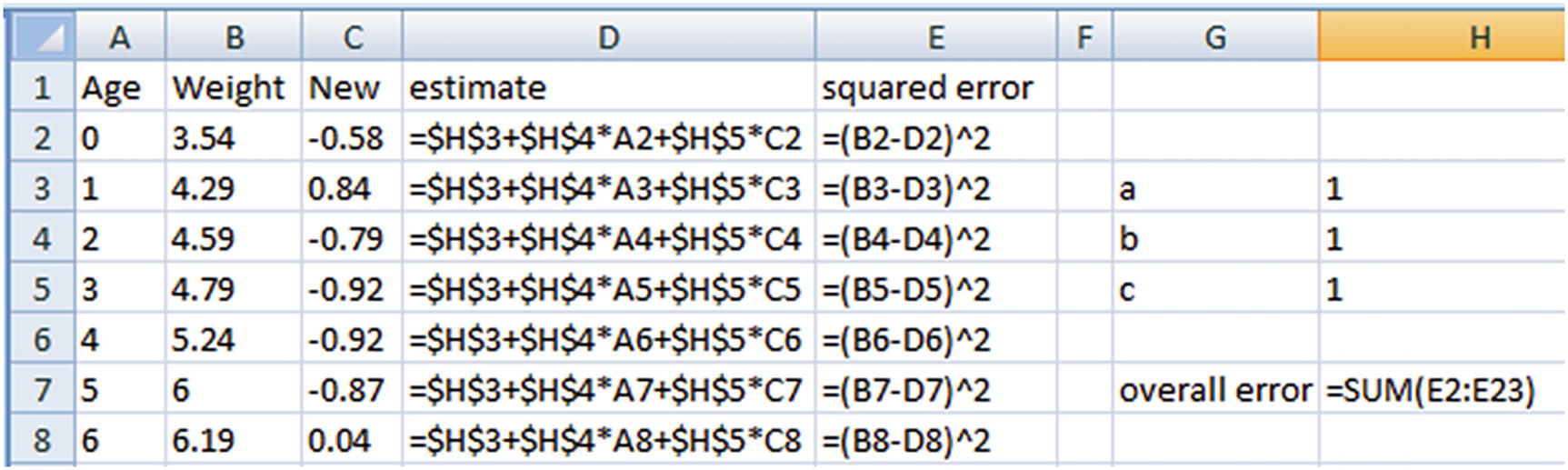
In this case, we would iterate through multiple values of a, b, and c—that is, cells H3, H4, and H5 that minimize the values of overall squared error.

Multivariate Linear Regression in R

Multivariate linear regression can be performed in R as follows (available as “Multivariate linear regression.R” in github):

# import file

data=read.csv("D:/Pro ML book/Linear regression/linear_multi_reg_example.csv")

# Build model

lm=glm(Weight~Age+New,data=data)

# summarize model

summary(lm)

../images/463052_1_En_2_Chapter/463052_1_En_2_Figk_HTML.jpg

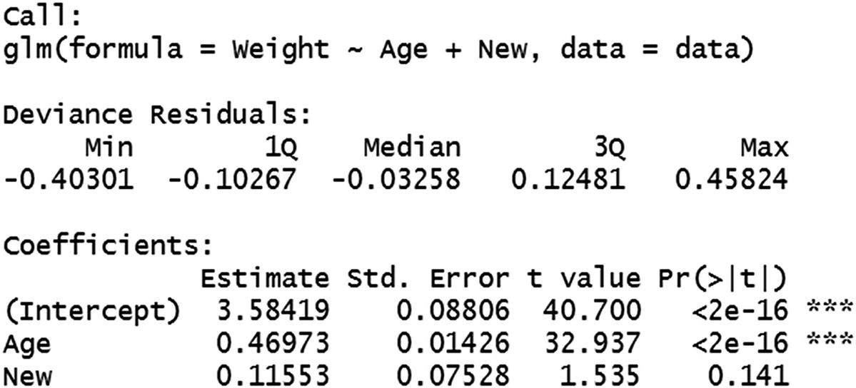
Note that we have specified multiple variables for regression by using the + symbol between the independent variables.

One interesting aspect we can note in the output would be that the New variable has a p-value that is greater than 0.05, and thus is an insignificant variable.

Typically, when a p-value is high, we test whether variable transformation or capping a variable would result in obtaining a low p-value. If none of the preceding techniques work, we might be better off excluding such variables.

Other details we can see here are calculated in a way similar to that of simple linear regression calculations in the previous sections.

Multivariate Linear Regression in Python

Similar to R, Python would also have a minor addition within the formula section to accommodate for multiple linear regression over simple linear regression:

# import relevant packages

# pandas package is used to import data

# statsmodels is used to inoke the functions that help in lm

import pandas as pd

import statsmodels.formula.api as smf

# import dataset

data = pd.read_csv('D:/Pro ML book/Linear regression/linear_multi_reg_example.csv')

# run least squares regression

est = smf.ols(formula='Weight~Age+New',data=data)

est2=est.fit()

print(est2.summary())

Issue of Having a Non-significant Variable in the Model

A variable is non-significant when the p-value is high. p-value is typically high when the standard error is high compared to coefficient value. When standard error is high, it is an indication that there is a high variance within the multiple coefficients generated for multiple samples. When we have a new dataset—that is, a test dataset (which is not seen by the model while building the model)—the coefficients do not necessarily generalize for the new dataset.

This would result in a higher RMSE for the test dataset when the non-significant variable is included in the model, and typically RMSE is lower when the non-significant variable is not included in building the model.

Issue of Multicollinearity

One of the major issues to take care of while building a multivariate model is when the independent variables may be related to each other. This phenomenon is called multicollinearity . For example, in the ice cream example, if ice cream prices increase by 20% on weekends, the two independent variables (price and weekend flag) are correlated with each other. In such cases, one needs to be careful when interpreting the result—the assumption that the rest of the variables remain constant does not hold true anymore.

For example, we cannot assume that the only variable that changes on a weekend is the weekend flag anymore; we must also take into consideration that price also changes on a weekend. The problem translates to, at a given temperature, if the day happens to be a weekend, sales increase by 0.2 units as it is a weekend, but decrease by 0.1 as prices are increased by 20% during a weekend—hence, the net effect of sales is +0.1 units on a weekend.

Mathematical Intuition of Multicollinearity

To get a glimpse of the issues involved in having variables that are correlated with each other among independent variables , consider the following example (code available as “issues with correlated independent variables.R” in github):

# import dataset

data=read.csv("D:/Pro ML book/linear_reg_example.csv")

# Creating a correlated variable

data$correlated_age = data$Age*0.5 + rnorm(nrow(data))*0.1

cor(data$Age,data$correlated_age)

# Building a linear regression

lm=glm(Weight~Age+correlated_age,data=data)

summary(lm)

../images/463052_1_En_2_Chapter/463052_1_En_2_Figl_HTML.jpg

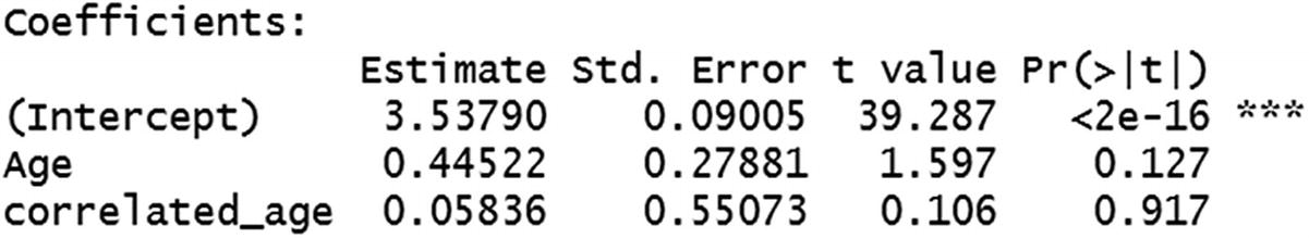
Note that, even though Age is a significant variable in predicting Weight in the earlier examples, when a correlated variable is present in the dataset, Age turns out to be a non-significant variable, because it has a high p-value.

The reason for high variance in the coefficients of Age and correlated_age by sample of data is that, more often than not, although the Age and correlated_age variables are correlated, the combination of age and correlated age (when treated as a single variable—say, the average of the two variables) would have less variance in coefficients.

Given that we are using two variables, depending on the sample, Age might have high coefficient, and correlated_age might have a low coefficient, and vice versa for some other samples, resulting in a high variance in coefficients for both variables by the sample chosen.

Further Points to Consider in Multivariate Linear Regression

It is not advisable for a regression to have very high coefficients: Although a regression can have high coefficients in some cases, in general, a high value of a coefficient results in a huge swing in the predicted value, even if the independent variable changes by 1 unit. For example, if sales is a function of price, where sales = 1,000,000 – 100,000 x price, a unit change of price can drastically reduce sales. In such cases, to avoid this problem, it is advisable to reduce the value of sales by changing it to log(sales) instead of sales, or normalize sales variable, or penalize the model for having high magnitude of weights through L1 and L2 regularizations (More on L1/ L2 regularizations in Chapter 7). This way, the a and b values in the equation remain small.
A regression should be built on considerable number of observations: In general, the higher the number of data points, more reliable the model is. Moreover, the higher the number of independent variables, the more data points to consider. If we have only two data points and two independent variables, we can always come up with an equation that is perfect for the two data points. But the generalization of the equation built on two data points only is questionable. In practice, it is advisable to have the number of data points be at least 100 times the number of independent variables.

The problem of low number of rows, or high number of columns, or both, brings us to the problem of adjusted R squared. As detailed earlier, the more independent variables in an equation, the higher the chances are of fitting it closest to the dependent variable, and thus a high R squared, even if the independent variables are non-significant. Thus, there should be a way of penalizing for having a high number of independent variables over a fixed set of data points. Adjusted R squared considers the number of independent variables used in an equation and penalizes for having more independent variables. The formula for adjusted R squared is as follows:

${R}_{adj}^2=1-\left[\frac{\left(1-{R}^2\right)\left(n-1\right)}{n-k-1}\right]$

where n is the number of data points in dataset and k is the number of independent variables in the dataset.

The model with the least adjusted R squared is generally the better model to go with.

Assumptions of Linear Regression

The assumptions of linear regression are as follows:

The independent variables must be linearly related to dependent variable : If the level of linearity changes over segment, a linear model is built per segment.
There should not be any outliers in values among independent variables : If there are any outliers, they should either be capped or a new variable needs to be created that flags the data points that are outliers.
Error values should be independent of each other: In a typical ordinary least squares method, the error values are distributed on both sides of the fitted line (that is, some predictions will be above actuals and some will be below actuals), as shown in Figure 2-4. A linear regression cannot have errors that are all on the same side, or that follow a pattern where low values of independent variable have error of one sign while high values of independent variable have error of the opposite sign.
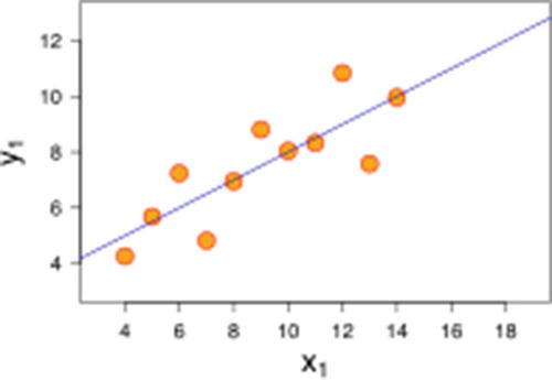Figure 2-4
Errors on both sides of the line
Homoscedasticity: Errors cannot get larger as the value of an independent variable increases. Error distribution should look more like a cylinder than a cone in linear regression (see Figure 2-5). In a practical scenario, we can think of the predicted value being on the x-axis and the actual value being on the y-axis.
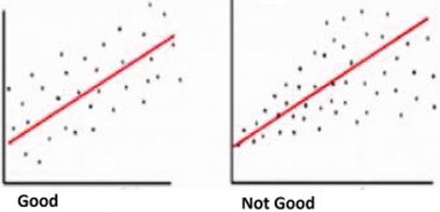Figure 2-5
Comparing error distributions
Errors should be normally distributed: There should be only a few data points that have high error. A majority of data points should have low error, and a few data points should have positive and negative error—that is, errors should be normally distributed (both to the left of overforecasting and to the right of underforecasting), as shown in Figure 2-6.
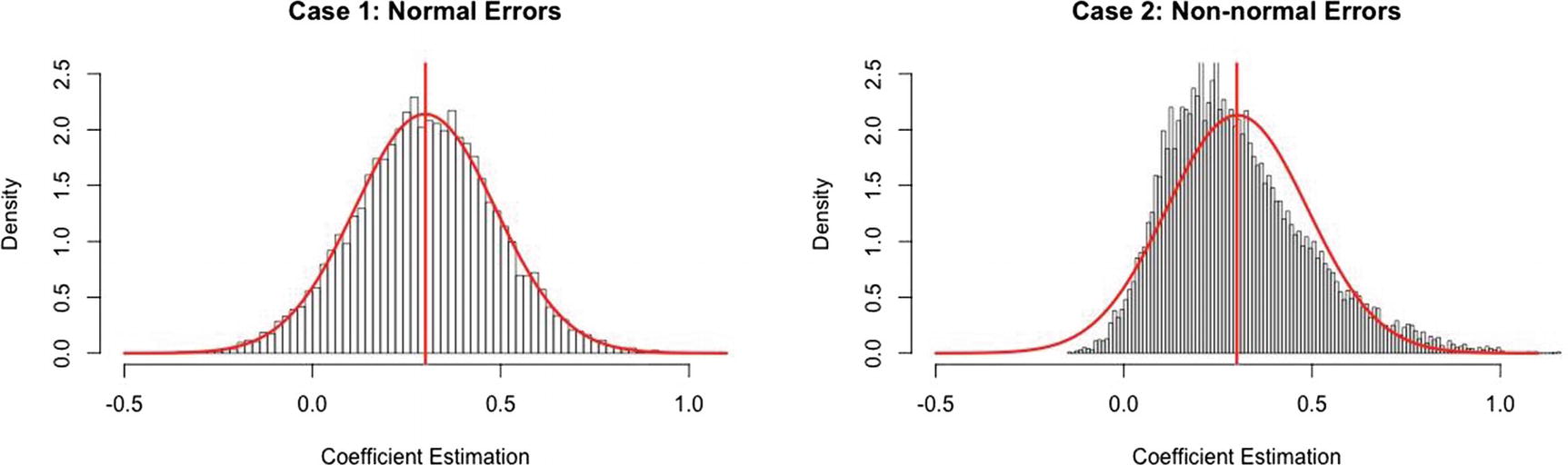Figure 2-6
Comparing curves

Note

In Figure 2-6, had we adjusted the bias (intercept) in the right-hand chart slightly, more observations would now surround zero error.

Summary

In this chapter, we have learned the following:

The sum of squared error (SSE) is the optimization based on which the coefficients in a linear regression are calculated.
Multicollinearity is an issue when multiple independent variables are correlated to each other.
p-value is an indicator of the significance of a variable in predicting a dependent variable.
For a linear regression to work, the five assumptions - that is, linear relation between dependent and independent variables, no outliers, error value independence, homoscedasticity, normal distribution of errors should be satisfied.

Previous Chapter

1. Basics of Machine Learning

Next Chapter

3. Logistic Regression

Table of Contents for Pro Machine Learning Algorithms : A Hands-On Approach to Implementing Algorithms in Python and R

2. Linear Regression

Introducing Linear Regression

Variables: Dependent and Independent

Correlation

Causation

Simple vs. Multivariate Linear Regression

Formalizing Simple Linear Regression

The Bias Term

The Slope

Solving a Simple Linear Regression

More General Way of Solving a Simple Linear Regression

Minimizing the Overall Sum of Squared Error

Solving the Formula

Working Details of Simple Linear Regression

Complicating Simple Linear Regression a Little

Arriving at Optimal Coefficient Values

Introducing Root Mean Squared Error

Running a Simple Linear Regression in R

Residuals

Note

Coefficients

SSE of Residuals (Residual Deviance)

Null Deviance

R Squared

F-statistic

Running a Simple Linear Regression in Python

Common Pitfalls of Simple Linear Regression

Multivariate Linear Regression

Working details of Multivariate Linear Regression

Multivariate Linear Regression in R

Multivariate Linear Regression in Python

Issue of Having a Non-significant Variable in the Model

Issue of Multicollinearity

Mathematical Intuition of Multicollinearity

Further Points to Consider in Multivariate Linear Regression

Assumptions of Linear Regression

Note

Summary

Table of Contents for
Pro Machine Learning Algorithms : A Hands-On Approach to Implementing Algorithms in Python and R