This chapter covers the compilation process. We divide it into three main stages: preprocessing, translation, and linking. Figure 5-1 shows an exemplary compilation process. There are two source files: first.asm and second.asm. Each is treated separately before linking stage.
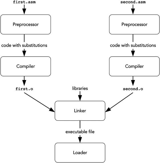
Figure 5-1. Compilation pipeline
Preprocessor transforms the program source to obtain other program in the same language. The transformations are usually substitutions of one string instead of others.
Compiler transforms each source file into a file with encoded machine instructions. However, such a file is not yet ready to be executed because it lacks the right connections with the other separately compiled files. We are talking about cases in which instructions address data or instructions, which are declared in other files.
Linker establishes connections between files and makes an executable file. After that, the program is ready to be run. Linkers operate with object files, whose typical formats are ELF (Executable and Linkable Format) and COFF (Common Object File Format).
Loader accepts an executable file. Such files usually have a structured view with metadata included. It then fills the fresh address space of a newborn process with its instructions, stack, globally defined data, and runtime code provided by the operating system.
5.1 Preprocessor
Each program is created as a text. The first stage of compilation is called preprocessing. During this stage, a special program is evaluating preprocessor directives found in the program source. According to them, textual substitutions are made. As a result we get a modified source code without preprocessor directives written in the same programming language. In this section we are going to discuss the usage of the NASM macro processor.
5.1.1 Simple Substitutions
One of the basic preprocessor directives is called %define. It performs a simple substitution.
Given the code shown in Listing 5-1, a preprocessor will substitute cat_count by 42 whenever it encounters such a substring in the program source.
Listing 5-1. define_cat_count.asm
%define cat_count 42mov rax, cat_count
To see the preprocessing results for an input file.asm, run nasm -E file.asm. It is often very useful for debug purposes. Let’s see the result in Listing 5-2 for the file in Listing 5-1.
Listing 5-2. define_cat_count_preprocessed.asm
%line 2+1 define_cat_count.asmmov rax, 42
The commands to declare substitutions are called macros . During a process called macro expansion their occurrences are replaced with pieces of text. The resulting text fragments are called macro instances. In Listing 5-2, a number 42 in line mov rax, cat_count is a macro instance. Names such as cat_count are often referred to as preprocessor symbols.
Redefinition
NASM allows you to redefine existing preprocessor symbols.
It is important that the preprocessor knows little to nothing about the programming language syntax. The latter defines valid language constructions.
For example, the code shown in Listing 5-3 is correct. It doesn’t matter if neither a nor b alone constitutes a valid assembly construction; as long as the final result of substitutions is syntactically valid, the compiler is fine with it.
Listing 5-3. macro_asm_parts.asm
%define a mov rax,%define b rbxa b
In another example, in higher-level languages, an if statement has a form of if (<expression>) then <statement> else <statement>. Macros can operate parts of this construction which on their own are not syntactically correct (e.g., a sole else <statement> clause). As long as the result is syntactically correct, the compiler will have no problems with it.
Contrarily, other types of macros exist, namely, syntactic macros, tied to the language structure and operating with its constructions. Such macros modify them in a structured way. Languages like LISP, OCaml, and Scala use syntactic macros.
Why are we using macros at all? Apart from automation, which we will see later, they provide mnemonics for pieces of code.1
For constants, it allows us distinguish occurrences of 42 which are used to count cats from those used to count dogs or whatever else. Otherwise, certain program modifications would be more painful and error prone, since we would have had to make more decisions based on what this specific number means.
For packs of language constructs, it provides us with a certain automatization just as subroutines do. Macros are expanded at compile time, while routines are executed in runtime. The choice is up to you.
For assembly, no optimizations are performed on programs. However, in higher-level languages people use global constant variables for that matter. A good compiler will substitute its occurrences with its value. A bad one, however, cannot be aware of optimizations, which can be the case when programming microcontrollers or applications for exotic operating systems. In such cases people often do a compiler’s job by using macros as in assembly language.
Style
It is a good practice to name all constants in your program.
In assembly and C people usually define global constants using macro definitions.
5.1.2 Substitutions with Arguments
Macros are better than that: they can have arguments . Listing 5-4 shows a simple macro with three arguments.
Listing 5-4. macro_simple_3arg.asm
%macro test 3dq %1dq %2dq %3%endmacro
Its action is simple: for each argument it will create a quad word data entry. As you see, arguments are referred by their indices starting at 1. When this macro is defined, a line test 666, 555, 444 will be replaced by those shown in Listing 5-5
Listing 5-5. macro_simple_3arg_inst.asm
dq 666dq 555dq 444
Question 68
Find more examples of %define and %macro usage in NASM documentation.
5.1.3 Simple Conditional Substitution
Macros in NASM support various conditionals . The simplest of them is %if. Listing 5-6 shows a minimal example.
Listing 5-6. macroif.asm
BITS 64%define x 5%if x == 10mov rax, 100%elif x == 15mov rax, 115%elif x == 200mov rax, 0%elsemov rax, rbx%endif
Listing 5-7 shows an instantiated macro. Remember, you can check the preprocessing result using nasm -E.
Listing 5-7. macroif_preprocessed.asm
%line 1+1 if.asm[bits 64]%line 15+1 if.asmmov rax, rbx
The condition is an expression similar to what you might see in high-level languages: arithmetics and logical conjectures (and, or, not).
5.1.4 Conditioning on Definition
It is possible to decide in compile time whether a part of file should be assembled or not. One of many %if counterparts is %ifdef. It works in a similar way, but the condition is satisfied if a certain preprocessor symbol is defined. An example shown in Listing 5-8 incorporates such a directive.
Listing 5-8. defining_in_cla.asm
%ifdef flaghellostring: db "Hello",0%endif
As you can see, the symbol flag is not defined here using %define directive. Thus, we have the line labeled by hellostring.
It is worth mentioning that preprocessor symbols can be defined directly when calling NASM thanks to -d key. For example, the macro condition in Listing 5-8 will be satisfied when NASM is called with -d myflag argument.
Question 69
Check the preprocessor output on file, shown in Listing 5-8.
In the next sections we are going to see more preprocessor directives similar to %if.
5.1.5 Conditioning on Text Identity
%ifidn is used to test if two text strings are equal (spacing differences are not taken into account). Depending on the comparison result the subsequent code will or will not be assembled.
This allows us to create very flexible macros which will depend, for example, on the argument name.
To illustrate, let’s create a pushr macro instruction (see Listing 5-9). It will function exactly the same way as a push assembly instruction but will also accept rip and rflags registers.
Listing 5-9. pushr.asm
%macro pushr 1%ifidn %1, rflagspushf%elsepush %1%endif%endmacropushr raxpushr rflags
Listing 5-10 shows what the two macros in Listing 5-9 become after instantiation.
Listing 5-10. pushr_preprocessed.asm
%line 8+1 pushr/pushr.asmpush raxpushf
As you can see, the macro adjusted its behavior based on the argument’s text representation. Notice that %else clauses are allowed just like for regular %if. To make the comparison case insensitive, use the %ifidni directive instead.
5.1.6 Conditioning on Argument Type
The NASM preprocessor is a bit aware of the assembly language elements (token types). It can distinguish quoted strings from numbers and identifiers. There is a triple of %if counterparts for this purpose: %ifid to check whether its argument is an identifier, %ifstr for a string check, and %ifnum to check whether it is a number or not.
Listing 5-11 shows an example of a macro , which prints either a number or a string (using an identifier). It uses several routines developed during the first assignment to calculate string length, output string, and output integer.
Listing 5-11. macro_arg_types.asm
%macro print 1%ifid %1mov rdi, %1call print_string%else%ifnum %1mov rdi, %1call print_uint%else%error "String literals are not supported yet"%endif%endif%endmacromyhello: db 'hello', 10, 0_start:print myhelloprint 42mov rax, 60syscall
The indentation is completely optional and is done for the sake of readability.
In case the argument is neither string nor identifier, we use the %error directive to force NASM into throwing an error. If we had used %fatal instead, we would have stopped assembling completely and any further errors would be ignored; a simple %error, however, will give NASM a chance to signal about following errors too before it stops processing input files.
Let’s observe the macro instantiations in Listing 5-12
Listing 5-12. macro_arg_types_preprocessed.asm
%line 73+1 macro_arg_types/macro_arg_types.asmmyhello: db 'hello', 10, 0_start:mov rdi, myhello%line 76+0 macro_arg_types/macro_arg_types.asmcall print_string%line 77+1 macro_arg_types/macro_arg_types.asm%line 77+0 macro_arg_types/macro_arg_types.asmmov rdi, 42call print_uint%line 78+1 macro_arg_types/macro_arg_types.asmmov rax, 60syscall
5.1.7 Evaluation Order: Define, xdefine, Assign
All programming languages have a notion of evaluation strategy. It describes the order of evaluation in complex expressions. How should we evaluate f (g(1), h(4))? Should we evaluate g(1) and h(4) first and then let f act on the results? Or should we inline g(1) and h(4) inside the body of f and defer their own evaluations until they are really needed?
Macros are evaluated by NASM macroprocessor, and they do have a complex structure, as any macro instantiation can include other macros to be instantiated. A fine tuning of evaluation order is possible, because NASM provides slightly different versions of macro definition directives, namely
%define for a deferred substitution. If macro body contains other macros, they will be expanded after the substitution.
%xdefine performs substitutions when being defined. Then the resulting string will be used in substitutions.
%assign is like %xdefine, but it also forces the evaluation of arithmetic expressions and throws an error if the computation result is not a number.
To better understand the subtle difference between %define and %xdefine take a look at the example shown in Listing 5-13.
Listing 5-13. defines. asm
%define i 1%define d i * 3%xdefine xd i * 3%assign a i * 3mov rax, dmov rax, xdmov rax, a; let's redefine i%define i 100mov rax, dmov rax, xdmov rax, a
Listing 5-14 shows the preprocessing result.
Listing 5-14. defines_preprocessed.asm
%line 2+1 defines.asm%line 6+1 defines.asmmov rax, 1 * 3mov rax, 1 * 3mov rax, 3mov rax, 100 * 3mov rax, 1 * 3mov rax, 3
The key differences are that
%define may change its value between instantiations if parts of it are redefined.
%xdefine has other macros on which it directly depends glued to it after being defined.
%assign forces evaluation and substitutes values. Where xdefine would have left you with the preprocessor symbol equal to 4+2+3, %assign will compute it and assign value 9 to it.
We will use the wonderful properties of %assign to show some magic after becoming familiar with macro repetitions.
5.1.8 Repetition
The times directive is executed after all macro definitions are fully expanded and thus cannot be used to repeat pieces of macros.
But there is another way NASM can make macro loops: by placing the loop body between %rep and %endrep directives. Loops can be executed only a fixed amount of times, specified as %rep argument. An example in Listing 5-15 shows how a preprocessor calculates a sum of integers from 1 to 10 and then uses this value to initialize a global variable result.
Listing 5-15. rep.asm
%assign x 1%assign a 0%rep 10%assign a x + a%assign x x + 1%endrepresult: dq a
After preprocessing the result value is correctly initialized to 55 (see Listing 5-16). You can check it manually.2
Listing 5-16. rep_preprocessed.asm
%line 7+1 rep/rep.asmresult: dq 55
We can use %exitrep to immediately leave the cycle. It is thus analogous to break instruction in high-level languages .
5.1.9 Example: Computing Prime Numbers
The macro shown in Listing 5-17 is used to produce a sieve of prime numbers. It means that it defines a static array of bytes, where each i-th byte is equal to 1 if and only if i is a prime number.
A prime number is a natural number greater than 1 such that it has no positive divisors other than 1 and itself.
The algorithm is simple:
0 and 1 are not primes.
2 is a prime number.
For each current up to limit we check whether no i from 2 up to n/2 is n’s divisor.
Listing 5-17. prime.asm
%assign limit 15is_prime: db 0, 0, 1%assign n 3%rep limit%assign current 1%assign i 1%rep n/2%assign i i+1%if n % i = 0%assign current 0%exitrep%endif%endrepdb current ; n%assign n n+1%endrep
By accessing the n-th element of the is_prime array we can find out whether n is a prime number or not. After preprocessing the following code in Listing 5-18 will be generated:
Listing 5-18. prime_preprocessed.asm
%line 2+1 prime/prime.asmis_prime: db 0, 0, 1%line 16+1 prime/prime.asmdb 1%line 16+0 prime/prime.asmdb 0db 1db 0db 1db 0db 0db 0db 1db 0db 1db 0db 0db 0db 1
By reading the i-th byte starting at is_prime we get 1 if i is prime; 0 otherwise.
Question 70
Modify the macro the way it would produce a bit table, taking eight times less space in memory. Add a function that will check number for primarily and return 0 or 1, based on this precomputed table.
Hint
for the macro you will probably have to copy and paste a lot.
5.1.10 Labels Inside Macros
There is not much we can do in assembly without labels. Using fixed label names inside macros is not quite common. When the macro is instantiated many times inside the same file, the multiply defined labels can produce clashes which stop compilation.
There is an option to use macro local labels, which is a label you cannot access outside current macro instantiation. In order to do that, you can prefix such label name with double percent, as follows: %%labelname. Each macro local label will get a random prefix, which will change between macro instances but will remain the same inside one instance. Listing 5-19 shows an example. Listing 5-20 contains the preprocessing results.
Listing 5-19. macro_local_labels.asm
%macro mymacro 0%%labelname:%%labelname:%endmacroMymacroMymacromymacro
The macro mymacro is instantiated three times . Each time the local label gets a unique name. The base name (after double percent) becomes prepended with a numerical prefix different in each instance. The first prefix is ..@0., the second is ..@1., and so on.
Listing 5-20. macro_local_labels_inst.asm
%line 5+1 macro_local_labels/macro_local_labels.asm..@0.labelname:%line 6+0 macro_local_labels/macro_local_labels.asm..@0.labelname:%line 7+1 macro_local_labels/macro_local_labels.asm..@1.labelname:%line 8+0 macro_local_labels/macro_local_labels.asm..@1.labelname:%line 9+1 macro_local_labels/macro_local_labels.asm..@2.labelname:%line 10+0 macro_local_labels/macro_local_labels.asm..@2.labelname:
5.1.11 Conclusion
You can think about macros as about a programming meta-language executed during compilation. It can do quite complex computations and is limited in two ways:
These computations cannot depend on user input (so they can only operate constants).
The cycles can be executed no more than a fixed amount of times. It means that while-like constructions are impossible to encode.
5.2 Translation
A compiler usually translates source code from one language into another language. In case of translation from high-level programming languages into machine code, this process incorporates multiple inner steps. During these stages we gradually push the code IR (Intermediate Representation) toward the target language. Each push of IR is closer to the target language. Right before producing assembly code the IR will be very close to assembly, so we can flush the assembly into a readable listing instead of encoding instructions.
Not only is translation a complex process, it also loses information about source code structure, so reconstructing readable high-level code from the assembly file is impossible.
A compiler works with atomic code entities called modules. A module usually corresponds to a code source file (but not a header or include file). Each module is compiled independently from the other modules. The object file is produced from each module. It contains binary encoded instructions but usually cannot be executed right away. There are several reasons.
For instance, the object file is completed separately from other files but refers to outside code and data. It is not yet clear whether that code or data will reside in memory, or the position of the object file itself.
The assembly language translation is quite straightforward because the correspondence between assembly mnemonics and machine instructions is almost one to one. Apart from label resolution there is not much nontrivial work. Thus, for now we will concentrate on the following compilation stage, namely, linking.
5.3 Linking
Let’s return to our first examples of assembly programs. To transform a “Hello, world!” program from source code to executable file, we used the following two commands:
> nasm -f elf64 -o hello.o hello.asm> ld -o hello hello.o
We used NASM first to produce an object file . Its format, elf64, was specified by the -f key. Then we used another program, ld (a linker), to produce a file ready to be executed. We will take this file format as an example to show you what the linker really does.
5.3.1 Executable and Linkable Format
ELF (Executable and Linkable Format) is a format for object files quite typical for *nix systems. We will limit ourselves to its 64-bit version.
ELF allows for three types of files.
Relocatable object files are .o-files, produced by compiler.
Relocation is a process of assigning definitive addresses to various program parts and changing the program code the way all links are attributed correctly. We are speaking about all kinds of memory accesses by absolute addresses. Relocation is needed, for example, when the program consists of multiple modules, which are referencing one another. The order in which they will be placed in memory is not yet fixed, so the absolute addresses are not determined. Linkers can combine these files to produce the next type of object files.
Executable object file can be loaded in memory and executed right away. It is essentially a structured storage for code, data, and utility information.
Shared object files can be loaded when needed by the main program. They are linked to it dynamically. In Windows OS these are well known dll-files; in *nix systems their names often end with .so.
The purpose of any linker is to make an executable (or shared) object file, given a set of relocatable ones. In order to do it, a linker must perform the following tasks:
Symbol resolution. Each time a symbol (function, variable) is dereferenced, a linker has to modify the object file and fill the instruction part, corresponding to the operand address, with the correct value.
5.3.1.1 Structure
An ELF file starts with the main header, which stores global meta-information.
See Listing 5-21 for a typical ELF header. The hello file is a result of compiling a “Hello, world!” program shown in Listing 2-4.
Listing 5-21. hello_elfheader ELF Header:
ELF Header:Magic: 7f 45 4c 46 02 01 01 00 00 00 00 00 00 00 00 00Class: ELF64Data: 2's complement, little endianVersion: 1 (current)OS/ABI: UNIX - System VABI Version: 0Type: EXEC (Executable file)Machine: Advanced Micro Devices X86-64Version: 0x1Entry point address: 0x4000b0Start of program headers: 64 (bytes into file)Start of section headers: 552 (bytes into file)Flags: 0x0Size of this header: 64 (bytes)Size of program headers: 56 (bytes)Number of program headers: 2Size of section headers: 64 (bytes)Number of section headers: 6Section header string table index: 3
ELF files then provide information about a program that can be observed from two points of view:
Linking view , consisting of sections.
It is described by section table, which is accessible through readelf -S.
Each section in turn can be:
Raw data to be loaded into memory.
Formatted metadata about other sections, used by loader (e.g., .bss ), linker (e.g., relocation tables ), or debugger (e.g., .line ).
Code and data are stored inside sections.
Execution view, consisting of segments.
It is described by a Program Header Table, which can be studied using readelf -l. We will take a closer look at it in section 5.3.5.
Each entry can describe
Some kind of information the system needs to execute the program.
An ELF segment, containing zero or more sections. They have the same set of permissions (read, write, execute) enforced by virtual memory. Each segment has a starting address and is loaded in a separate memory region, consisting of consecutive pages .
After revising Listing 5-21, we notice, that it describes precisely the position and dimensions of program headers and section headers.
We start with the sections view since the linker works mainly with them.
5.3.1.2 Sections in ELF Files
Assembly language allows manual section controls . NASM’s section corresponds to object file sections. You have already seen a couple of those, namely, .text and .data. The list of the most used sections follows; the full list can be found in [24].
.text stores machine instructions.
.rodata stores read only data.
.data stores initialized global variables.
.bss stores readable and writable global variables, initialized to zero. There is no need to dump their contents into an object file as they are all filled with zeros anyway. Instead, a total section size is stored. An operating system may know faster ways of initializing such memory than zeroing it manually.
In assembly, you can put data here by placing resb, resw, and similar directives after the section .bss.
.rel.text stores relocation table for the .text section. It is used to memorize places where a linker should modify .text after choosing the loading address for this specific object file.
.rel.data stores a relocation table for data referenced in module .
.debug stores a symbol table used to debug program. If the program was written in C or C++, it will store information not only about global variables (as .symtab does) but also about local variables.
.line defines correspondence with pieces of code and line numbers in source code. We need it because the correspondence between lines of source code in higher-level languages and assembly instructions is not straightforward. This information allows one to debug a program in a higher-level language line by line.
.strtab stores character strings. It is like an array of strings. Other sections, such, as .symtab and .debug , use not immediate strings but their indices in .strtab .
.symtab stores a symbol table. Whenever a programmer defines a label, NASM will create a symbol for it.3 This table also stores utility information, which we are going to examine later.
Now that we have a general understanding of the ELF file linking view, we will observe some examples to show particularities of three different ELF file types.
5.3.2 Relocatable Object Files
Let’s investigate an object file, obtained by compiling a simple program, shown in Listing 5-22.
Listing 5-22. symbols.asm
section .datadatavar1: dq 1488datavar2: dq 42section .bssbssvar1: resq 4*1024*1024bssvar2: resq 1section .textextern somewhereglobal _startmov rax, datavar1mov rax, bssvar1mov rax, bssvar2mov rdx, datavar2_start:jmp _startrettextlabel: dq 0
This program uses extern and global directives to mark symbols in a different way. These two directives control the creation of a symbol table. By default, all symbols are local to the current module. extern defines a symbol that is defined in other modules but referenced in the current one. On the other hand, global defines a globally available symbol that other modules can refer to by defining it as extern inside them.
Avoid confusion
Do not confuse global and local symbols with global and local labels!
The GNU binutils is a collection of binary tools used to work with object files. It includes several tools used to explore the object file contents. Several of them are of particular interest for us.
If you only need to look up the symbol table, use nm.
Use objdump as a universal tool to display general information about an object file. In addition to ELF, it does support other object file formats.
If you know that the file is in ELF format, readelf is often the best and most informative choice.
Let’s feed this program to objdump to produce the results shown in Listing 5-23.
Listing 5-23. Symbols
> nasm -f elf64 main.asm && objdump -tf -m intel main.omain.o: file format elf64-x86-64architecture: i386:x86-64, flags 0x00000011:HAS_RELOC, HAS_SYMSstart address 0x0000000000000000SYMBOL TABLE:0000000000000000 l df *ABS* 0000000000000000 main.asm0000000000000000 l d .data 0000000000000000 .data0000000000000000 l d .bss 0000000000000000 .bss0000000000000000 l d .text 0000000000000000 .text0000000000000000 l .data 0000000000000000 datavar10000000000000008 l .data 0000000000000000 datavar20000000000000000 l .bss 0000000000000000 bssvar10000000002000000 l .bss 0000000000000000 bssvar20000000000000029 l .text 0000000000000000 textlabel0000000000000000 *UND* 0000000000000000 somewhere0000000000000028 g .text 0000000000000000 _start
We are shown a symbol table, where each symbol is annotated with useful information. What do its columns mean?
Virtual address of the given symbol. For now we do not know the section starting addresses, so all virtual addresses are given relative to section start. For example, datavar1 is the first variable stored in .data, its address is 0, and its size is 8 bytes. The second variable, datavar2, is located in the same section with a greater offset of 8, next to datavar1. As somewhere is defined as extern, it is obviously located in some other module, so for now its address has no meaning and is left zero.
A string of seven letters and spaces; each letter characterizes a symbol in some way. Some of them are of interest to us.
l, g,- – local, global, or neither.
…
…
…
I,- – a link to another symbol or an ordinary symbol.
d, D,- – debug symbol, dynamic symbol, or an ordinary symbol.
F, f, O,- – function name, file name, object name, or an ordinary symbol.
What section does this label correspond to? *UND* for unknown section (symbol is referenced, but not defined here), *ABS* means no section at all.
Usually, this number shows an alignment (or its absence).
Symbol name.
For example, let’s investigate the first symbol shown in Listing 5-23. It is
f a file name,
d only necessary for debug purposes,
l local to this module.
The global label _start (which is also an entry point ) is marked with the letter g in the second column.
Note
Symbol names are case sensitive: _start and _STaRT are different.
As the addresses in the symbol table are not yet the real virtual addresses but ones relative to sections, we might ask ourselves: how do these look in machine code? NASM has already performed its duty, and the machine instructions should be assembled. We can look inside interesting sections of object files by invoking objdump with parameters -D (disassemble) and, optionally, -M intel-mnemonic (to make it show Intel-style syntax rather than AT&T one). Listing 5-24 shows the results.
How to read disassembly dumps
The left column usually is the absolute address where the data will be loaded. Before linking, it is an address relative to the section start.
The second column shows raw bytes as hexadecimal numbers.
The third column can contain the results of disassembling the assembly command mnemonics.
Listing 5-24. objdump_d
> objdump -D -M intel-mnemonic main.omain.o: file format elf64-x86-64Disassembly of section .data:0000000000000000 <datavar1>: ...0000000000000008 <datavar2>: ...Disassembly of section .bss:0000000000000000 <bssvar1>: ...0000000002000000 <bssvar2>: ...Disassembly of section .text:0000000000000000 <_start-0x28>:0: 48 b8 00 00 00 00 00 movabs rax,0x07: 00 00 00a: 48 b8 00 00 00 00 00 movabs rax,0x011: 00 00 0014: 48 b8 00 00 00 00 00 movabs rax,0x01b: 00 00 001e: 48 ba 00 00 00 00 00 movabs rdx,0x025: 00 00 000000000000000028 <_start>:28: c3 ret0000000000000029 <textlabel>:
The mov operand in section .text with offsets 0 and 14 relative to section start should be datavar1 address , but it is equal to zero! The same thing happened with bssvar. It means that the linker has to change compiled machine code, filling the right absolute addresses in instruction arguments. To achieve that, for each symbol all references to it are remembered in relocation table . As soon as the linker understands what its true virtual address will be, it goes through the list of symbol occurrences and fills in the holes.
A separate relocation table exists for each section in need of one.
To see the relocation tables use readelf --relocs. See Listing 5-25.
Listing 5-25. readelf_relocs
> readelf --relocs main.oRelocation section '.rela.text' at offset 0x440 contains 4 entries:Offset Info Type Sym. Value Name+Addend000000000002 000200000001 R_X86_64_64 0000000000000000 .data + 000000000000c 000300000001 R_X86_64_64 0000000000000000 .bss + 0000000000016 000300000001 R_X86_64_64 0000000000000000 .bss + 2000000000000000020 000200000001 R_X86_64_64 0000000000000000 .data + 8
An alternative way to display the symbol table is to use a more lightweight and minimalistic nm utility. For each symbol it shows the symbol’s virtual address, type, and name. Note that the type flag is in different format compared to objdump. See Listing 5-26 for a minimal example.
Listing 5-26. nm
> nm main.o0000000000000000 b bssvar0000000000000000 d datavarU somewhere000000000000000a T _start000000000000000b t textlabel
5.3.3 Executable Object Files
The second type of object file can be executed right away. It retains its structure, but the addresses are now bound to exact values.
We shall take a look at another example, shown in Listing 5-27. It includes two global variables, somewhere and private, one of which is available to all modules (marked global). Additionally, a symbol func is marked as global.
Listing 5-27. executable_object.asm
global somewhereglobal funcsection .datasomewhere: dq 999private: dq 666section .textfunc:mov rax, somewhereret
We are going to compile it as usual using nasm -f elf64, and then link it using ld with the previous object file, obtained by compiling the file shown in Listing 5-22. Listing 5-28 shows the changes in objdump output.
Listing 5-28. objdump_tf
> nasm -f elf64 symbols.asm> nasm -f elf64 executable_object.asm> ld symbols.o executable_object.o -o main> objdump -tf mainmain: file format elf64-x86-64architecture: i386:x86-64, flags 0x00000112:EXEC_P, HAS_SYMS, D_PAGEDstart address 0x0000000000000000SYMBOL TABLE:00000000004000b0 l d .code 0000000000000000 .code00000000006000bc l d .data 0000000000000000 .data0000000000000000 l df *ABS* 0000000000000000 executable_object.asm00000000006000c4 l .data 0000000000000000 private00000000006000bc g .data 0000000000000000 somewhere0000000000000000 *UND* 0000000000000000 _start00000000006000cc g .data 0000000000000000 __bss_start00000000004000b0 g F .code 0000000000000000 func00000000006000cc g .data 0000000000000000 _edata00000000006000d0 g .data 0000000000000000 _end
The flags are different : now the file can be executed (EXEC_P); there are no more relocation tables (the HAS_RELOC flag is cleared). Virtual addresses are now intact, and so are addresses in code. This file is ready to be loaded and executed. It retains a symbol table, and if you want to cut it out making the executable smaller, use the strip utility.
Question 71
Why does ld issue a warning if _start is not marked global? Look the entry point address in this case by using readelf with appropriate arguments.
Question 72
Find out the ld option to automatically strip the symbol table after linking.
5.3.4 Dynamic Libraries
Almost every program uses code from libraries. There are two types of libraries : static and dynamic.
Static libraries consist of several relocatable object files. These are linked to the main program and are merged with the result executable file.
In the Windows world, these files have an extension .lib.
In the Unix world, these are either .o files or .a archives holding several .o files inside.
Dynamic libraries are also known as shared object files the third of three object file types we have defined previously.
They are linked with the program during its execution.
In the Windows world, these are the infamous .dll files.
In the Unix world, these files have an .so extension (shared objects).
While static libraries are just undercooked executables without entry points, dynamic libraries have some differences which we are going to look at now.
Dynamic libraries are loaded when they are needed. As they are object files on their own, they have all kind of meta-information about which code they provide for external usage. This information is used by a loader to determine the exact addresses of exported functions and data.
Dynamic libraries can be shipped separately and updated independently. It is both good and bad. While the library manufacturer can provide bug fixes, he can also break backward compatibility by, for example, changing functions arguments, effectively shipping a delayed action mine.
A program can work with any amount of shared libraries . Such libraries should be loadable at any address. Otherwise they would be stuck at the same address, which puts us in exactly the same situation as when we are trying to execute multiple programs in the same physical memory address space. There are two ways to achieve that:
We can perform a relocation in runtime, when the library is being loaded. However, it steals a very attractive feature from us: the possibility to reuse library code in physical memory without its duplication when several processes are using it. If each process performs library relocation to a different address, the corresponding pages become patched with different address values and thus become different for different processes.
Effectively the .data section would be relocated anyway because of its mutable nature. Renouncing global variables allows us to throw away both the section and the need to relocate it.
Another problem is that .text section must be left writable in order to perform its modification during the relocation process. It introduces certain security risks, leaving its modification possible by malicious code. Moreover, changing .text of every shared object when multiple libraries are required for an executable to run can take a great deal of time.
We can write PIC (Position Independent Code). It is now possible to write code which can be executed no matter where it resides in memory. For that we have to get rid of absolute addresses completely. These days processors support rip-relative addressing, like mov rax, [rip + 13]. This feature facilitates PIC generation.
This technique allows for .text section sharing. Today programmers are strongly encouraged to use PIC instead of relocations.
Note
Whenever you are using non-constant global variables, you prevent your code from being reenterable, that is, being executable inside multiple threads simultaneously without changes. Consequently, you will have difficulties reusing it in a shared library. It is one of many arguments against a global mutable state in program.
Dynamic libraries spare disk space and memory. Remember that pages may be either marked private or shared among several processes. If a library is used by multiple processes, most parts of it are not duplicated in physical memory.
We will show you how to build a minimal shared object now. However, we will defer the explanation of things like Global Offset Tables and Procedure Linkage Tables until Chapter 15.
Listing 5-29 shows minimal shared object contents. Notice the external symbol _GLOBAL_OFFSET_TABLE and :function specification for the global symbol func. Listing 5-30 shows a minimal launcher that calls a function in a shared object file and exits correctly.
Listing 5-29. libso.asm
Extern _GLOBAL_OFFSET_TABLE_global func:functionsection .rodatamessage: db "Shared object wrote this", 10, 0section .textfunc:mov rax, 1mov rdi, 1mov rsi, messagemov rdx, 14syscallret
Listing 5-30. libso_main.asm
global _startextern funcsection .text_start:mov rdi, 10call funcmov rdi, raxmov rax, 60syscall
Listing 5-31 shows build commands and two views of an ELF file.
Notice that dynamic library has more specific sections such as .dynsym. Sections .hash, .dynsym, and .dynstr are necessary for relocation.
.dynsym stores symbols visible from outside the library.
.hash is a hash table, needed to decrease the symbol search time for .dynsym.
. dynstr stores strings, requested by their indices from .dynsym.
Listing 5-31. libso
> nasm -f elf64 -o main.o main.asm> nasm -f elf64 -o libso.o libso.asm> ld -o main main.o -d libso.so> ld -shared -o libso.so libso.o --dynamic-linker=/lib64/ld-linux-x86-64.so.2> readelf -S libso.soThere are 13 section headers, starting at offset 0x5a0:Section Headers:[Nr] Name Type Address OffsetSize EntSize Flags Link Info Align[ 0] NULL 0000000000000000 000000000000000000000000 0000000000000000 0 0 0[ 1] .hash HASH 00000000000000e8 000000e8000000000000002c 0000000000000004 A 2 0 8[ 2] .dynsym DYNSYM 0000000000000118 000001180000000000000090 0000000000000018 A 3 2 8[ 3] .dynstr STRTAB 00000000000001a8 000001a8000000000000001e 0000000000000000 A 0 0 1[ 4] .rela.dyn RELA 00000000000001c8 000001c80000000000000018 0000000000000018 A 2 0 8[ 5] .text PROGBITS 00000000000001e0 000001e0000000000000001c 0000000000000000 AX 0 0 16[ 6] .rodata PROGBITS 00000000000001fc 000001fc000000000000001a 0000000000000000 A 0 0 4[ 7] .eh_frame PROGBITS 0000000000000218 000002180000000000000000 0000000000000000 A 0 0 8[ 8] .dynamic DYNAMIC 0000000000200218 0000021800000000000000f0 0000000000000010 WA 3 0 8[ 9] .got.plt PROGBITS 0000000000200308 000003080000000000000018 0000000000000008 WA 0 0 8[10] .shstrtab STRTAB 0000000000000000 000003200000000000000065 0000000000000000 0 0 1[11] .symtab SYMTAB 0000000000000000 0000038800000000000001c8 0000000000000018 12 15 8[12] .strtab STRTAB 0000000000000000 00000550000000000000004f 0000000000000000 0 0 1Key to Flags:W (write), A (alloc), X (execute), M (merge), S (strings), l (large)I (info), L (link order), G (group), T (TLS), E (exclude), x (unknown)O (extra OS processing required) o (OS specific), p (processor specific)> readelf -S mainThere are 14 section headers, starting at offset 0x650:Section Headers:[Nr] Name Type Address OffsetSize EntSize Flags Link Info Align[ 0] NULL 0000000000000000 000000000000000000000000 0000000000000000 0 0 0[ 1] .interp PROGBITS 0000000000400158 00000158000000000000000f 0000000000000000 A 0 0 1[ 2] .hash HASH 0000000000400168 000001680000000000000028 0000000000000004 A 3 0 8[ 3] .dynsym DYNSYM 0000000000400190 000001900000000000000078 0000000000000018 A 4 1 8[ 4] .dynstr STRTAB 0000000000400208 000002080000000000000027 0000000000000000 A 0 0 1[ 5] .rela.plt RELA 0000000000400230 000002300000000000000018 0000000000000018 AI 3 6 8[ 6] .plt PROGBITS 0000000000400250 000002500000000000000020 0000000000000010 AX 0 0 16[ 7] .text PROGBITS 0000000000400270 000002700000000000000014 0000000000000000 AX 0 0 16[ 8] .eh_frame PROGBITS 0000000000400288 000002880000000000000000 0000000000000000 A 0 0 8[ 9] .dynamic DYNAMIC 0000000000600288 000002880000000000000110 0000000000000010 WA 4 0 8[10] .got.plt PROGBITS 0000000000600398 000003980000000000000020 0000000000000008 WA 0 0 8[11] .shstrtab STRTAB 0000000000000000 000003b80000000000000065 0000000000000000 0 0 1[12] .symtab SYMTAB 0000000000000000 0000042000000000000001e0 0000000000000018 13 15 8[13] .strtab STRTAB 0000000000000000 00000600000000000000004d 0000000000000000 0 0 1
Question 73
Study the symbol tables for an obtained shared object using readelf --dyn-syms and objdump -ft.
Question 74
What is the meaning behind the environment variable LD_LIBRARY_PATH?
Question 75
Separate the first assignment into two modules. The first module will store all functions defined in lib.inc. The second will have the entry point and will call some of these functions.
Question 76
Take one of the standard Linux utilities (from coreutils). Study its object file structure using readelf and objdump.
The things we observed in this section apply in most situations. However, there is a bigger picture of different code models that affect the addressing. We will dive into those details in Chapter 15 after getting more familiar with assembly and C. There we will also revise the dynamic libraries again and introduce the notions of Global Offset Table and Procedure Linkage Table.
5.3.5 Loader
Loader is a part of the operating system that prepares executable file for execution. It includes mapping its relevant sections into memory, initializing .bss , and sometimes mapping other files from disk.
The program headers for a file symbols.asm, shown in Listing 5-22, are shown in Listing 5-32.
Listing 5-32. symbols_pht
> nasm -f elf64 symbols.asm> nasm -f elf64 executable_object.asm> ld symbols.o executable_object.o -o main> readelf -l mainElf file type is EXEC (Executable file)Entry point 0x4000d8There are 2 program headers, starting at offset 64Program Headers:Type Offset VirtAddr PhysAddrFileSiz MemSiz Flags AlignLOAD 0x0000000000000000 0x0000000000400000 0x00000000004000000x00000000000000e3 0x00000000000000e3 R E 200000LOAD 0x00000000000000e4 0x00000000006000e4 0x00000000006000e40x0000000000000010 0x000000000200001c RW 200000Section to Segment mapping:Segment Sections...00 .text01 .data .bss
The table tells us that two segments are present.
00 segment
Is loaded at 0x400000 aligned at 0x200000.
Contains section .text.
Can be executed and can be read. Cannot be written to (so you cannot overwrite code).
01 segment
Is loaded at 0x6000e4 aligned to 0x200000.
Can be read and written to.
Alignment means that the actual address will be the closest one to the start, divisible by 0x200000.
Thanks to virtual memory, you can load all programs at the same starting address. Usually it is 0x400000.
There are some important observations to be made:
Assembly sections with similar names, defined in different files, are merged.
A relocation table is not needed in a pure executable file. Relocations partially remain for shared objects.
Let’s launch the resulting file and see its /proc/<pid>/maps file as we did in Chapter 4. Listing 5-33 shows its sample contents. The executable is crafted to loop infinitely.
Listing 5-33. symbols_maps
00400000-00401000 r-xp 00000000 08:01 1176842/home/sayon/repos/spbook/en/listings/chap5/main00600000-00601000 rwxp 00000000 08:01 1176842/home/sayon/repos/spbook/en/listings/chap5/main00601000-02601000 rwxp 00000000 00:00 07ffe19cf2000-7ffe19d13000 rwxp 00000000 00:00 0[stack]7ffe19d3e000-7ffe19d40000 r-xp 00000000 00:00 0[vdso]7ffe19d40000-7ffe19d42000 r--p 00000000 00:00 0[vvar]ffffffffff600000-ffffffffff601000 r-xp 00000000 00:00 0[vsyscall]
As we see, the program header is telling us the truth about section placement.
Note
In some cases, you will find that the linker needs to be finely tuned. The section loading addresses and relative placement can be adjusted by using linker scripts, which describe the resulting file. Such cases usually occur when you are programming an operating system or a microcontroller firmware. This topic is beyond the scope of this book, but we recommend that you look at [4] in case you encounter such a need.
5.4 Assignment: Dictionary
This assignment will further advance us to a working Forth interpreter. Some things about it might seem forced, like the macro design, but it will make a good foundation for an interpreter we are going to do later.
Our task is to implement a dictionary . It will provide a correspondence between keys and values. Each entry contains the address of the next entry, a key, and a value. Keys and values in our case are null-terminated strings.
The dictionary entries form a data structure are called a linked list. An empty list is represented by a null pointer, equal to zero. A non-empty list is a pointer to its first element. Each element holds some kind of value and a pointer to the next element (or zero, if it is the last element).
Listing 5-34 shows an exemplary linked list, holding elements 100, 200, and 300. It can be referred to by a pointer to its first element, that is, x1.
Listing 5-34. linked_list_ex.asm
section .datax1:dq x2dq 100x2:dq x3dq 200x3:dq 0dq 300
Linked lists are often useful in situations that have numerous insertions and removals in the middle of the list. Accessing elements by index, however, is hard because it does not boil down to simple pointer addition. Linked list elements’ mutual positions in flat memory are usually not predictable.
In this assignment the dictionary will be constructed statically as a list and each newly defined element will be prepended to it. You have to use macros with local labels and symbol redefinition to automatize the linked list creation. We explicitly instruct you to make a macro colon with two arguments, where the first will hold a dictionary key string and the second will hold the internal element representation name. This differentiation is needed because key strings can sometimes contain characters which are not parts of valid label names (space, punctuation, arithmetic signs, etc.). Listing 5-35 shows an example of such a dictionary.
Listing 5-35. linked_list_ex_macro.asm
section .datacolon "third word", third_worddb "third word explanation", 0colon "second word", second_worddb "second word explanation", 0colon "first word", first_worddb "first word explanation", 0
The assignment will contain the following files:
main.asm
lib.asm
dict.asm
colon.inc
Follow these steps to complete the assignment:
Make a separate assembly file containing functions that you have already written in the first assignment. We will call it lib.o.
Do not forget to mark all necessary labels global, otherwise they won’t be visible outside of this object file!
Create a file colon.inc and define a colon macro there to create dictionary words.
This macro will take two arguments:
Dictionary key (inside quotes).
Assembly label name. Keys can contain spaces and other characters, which are not allowed in label names.
Each entry should start with a pointer to the next entry, then hold a key as a null-terminated string. The content is then directly described by a programmer—for example, using db directives, as in the example shown in Listing 5-35.
Create a function find_word inside a new file dict.asm. It accepts two arguments :
A pointer to a null terminated key string.
A pointer to the last word in the dictionary. Having a pointer to the last word defined, we can follow the consecutive links to enumerate all words in the dictionary.
find_ word will loop through the whole dictionary, comparing a given key with each key in dictionary. If the record is not found, it returns zero; otherwise it returns record address.
A separate include file words.inc to define dictionary words using the colon macro. Include it in main.asm.
A simple _start function. It should perform the following actions:
Read the input string in a buffer of maximum 255 characters long.
Try to find this key in dictionary. If found, print the corresponding value. If not, print an error message.
Do not forget: all error messages should be written in stderr rather than stdout!
We ship a set of stub files (see Section 2.1 “Setting Up the Environment”); you are free to use them. An additional Makefile describes the building process; type make in the assignment directory to build an executable file main. A quick tutorial to the GNU Make system is available in Appendix B.
As in the first assignment , there is a test.py file to perform automated tests.
5.5 Summary
In this chapter we have looked at the different compilation stages. We have studied the NASM macroprocessor in detail and learned conditionals and loops. Then we talked about three object file types: relocatable, executable, and shared. We elaborated the ELF file structure and observed the relocation process performed by the linker. We have touched on the shared object files, and we will revisit them again in the Chapter 15.
Question 77
What is the linked list?
Question 78
What are the compilation stages?
Question 79
What is preprocessing?
Question 80
What is a macro instantiation?
Question 81
What is the %define directive?
Question 82
What is the %macro directive?
Question 83
What is the difference between %define, %xdefine, and %assign?
Question 84
Why do we need the %% operator inside macro?
Question 85
What types of conditions are supported by NASM macroprocessor? Which directives are used for it?
Question 86
What are the three types of ELF object files?
Question 87
What kinds of headers are present in an ELF file?
Question 88
What is relocation?
Question 89
What sections can be present in ELF files?
Question 90
What is a symbol table? What kind of information does it store?
Question 91
Is there a connection between sections and segments?
Question 92
Is there a connection between assembly sections and ELF sections?
Question 93
What symbol marks the program entry point?
Question 94
Which are the two different kind of libraries?
Question 95
Is there a difference between a static library and a relocatable object file?
