Sparse matrices are rarely discussed, if at all, due to the relative complexity of implementation and maintenance; however, they may be a very convenient and useful instrument in certain cases. Basically, sparse matrices are conceptually very close to arrays, but they're much more efficient when working with sparse data as they allow memory savings, which in turn allows the processing of much larger amounts of data.

Let's take astrophotography as an example. For those of us not familiar with the subject, amateur astrophotography means plugging your digital camera into a telescope, selecting a region in the night sky, and taking pictures. However, since pictures are taken at night time without a flashlight or any other aid (it would be silly to try to light celestial objects with a flashlight anyway), one has to take dozens of pictures of the same object and then stack the images together using a specific algorithm. In this case, there are two major problems:

• Noise reduction
• Image alignment

Lacking professional equipment (meaning not having a huge telescope with a cooled CCD or CMOS matrix), one faces the problem of noise. The longer the exposition, the more noise in the final image. Of course, there are numerous algorithms for noise reduction, but sometimes, a real celestial object may mistakenly be treated as noise and be removed by the noise reduction algorithm. Therefore, it is a good idea to process each image and detect potential celestial objects. If certain "light", which otherwise may be considered as noise, is present in at least 80% of images (it is hard to believe that any noise would have survived for such a long time without any changes, unless we are talking about dead pixels), then its area needs different treatment.

However, in order to process an image, we need to make a decision on how to store the result. We, of course, may use an array of structures describing each and every pixel, but that would be too expensive by means of the memory required for such operation. On the other hand, even if we take a picture of the highly populated area of the night sky, the area occupied by celestial objects would be significantly smaller than the "empty" space. Instead, we may divide an image into smaller areas, analyze certain characteristics of those smaller regions, and only take into consideration those that seem to be populated. The following figure presents the idea:

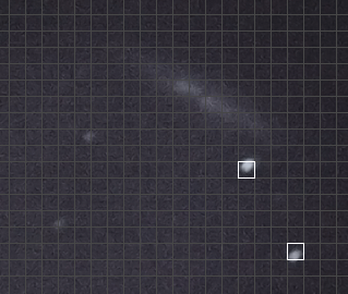
The figure (which shows the Messier 82 object, also known as Cigar Galaxy) is divided into 396 smaller regions (a matrix of 22 x 18 regions, 15 x 15 pixels each). Each region may be described by its luminosity, noise ratio, and many other aspects, including its location on the figure, meaning that it may occupy quite a sensible amount of memory. Having this data stored in a two-dimensional array with more than 30 images simultaneously may result in megabytes, of meaningless data. As the image shows, there are only two regions of interest, which together form about 0.5% (which fits the definition of sparse data more than perfectly), meaning that if we choose to use arrays, we waste 99.5% of the used memory.

Utilizing sparse matrices, we may reduce the usage of memory to the minimum required to store important data. In this particular case, we would have a linked list of 22 column header nodes, 18 row header nodes, and only 2 nodes for data. The following is a very rough example of such an arrangement:

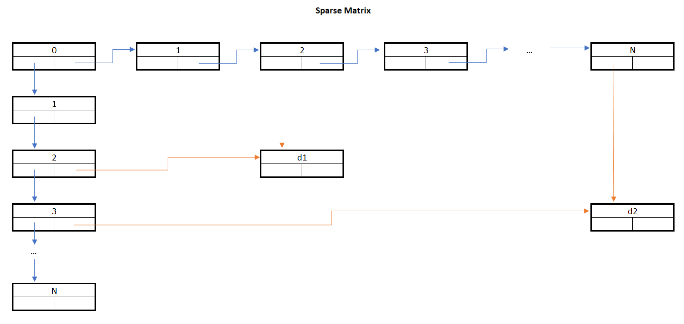
The preceding example is very rough; in reality, the implementation would contain a few other links. For example, empty column header nodes would have their down pointer point to themselves, and empty row headers would have their right pointers point to themselves, too. The last data node in a row would have its right pointer pointing to the row header node, and the same applies to the last data node in a column having its down pointer pointing to the column header node.