k-Shape

One of the state-of-the-art approaches to time series clustering that meets this criteria is k-Shape, which was first introduced at ACM SIGMOD in 2015 by John Paparrizos and Luis Gravano.¹

k-Shape uses a distance measure that is invariant to scaling and shifting to preserve the shapes of time-series sequencies while comparing them. Specifically, k-Shape uses a normalized version of cross-correlation to compute cluster centroids and then, in every iteration, updates the assignment of time series to these clusters.

In addition to being invariant to scaling and shifting, k-Shape is domain-independent and scalable, requiring minimal parameter tuning. Its iterative refinement procedures scales linearly in the number of sequences. These characteristics have led it to become one of the most powerful time series clustering algorithms available today.

By this point, it should be clear that k-Shape operates similarly to k-means - both algorithms use an iterative approach to assign data to groups based on the distance between the data and the centroid of the nearest group. The critical difference is in how k-Shape calculates distances - it uses shaped-based distance that relies on cross-correlations.

Data Preparation

Let’s begin by loading the necessary libraries.

'''Main'''
import numpy as np
import pandas as pd
import os, time, re
import pickle, gzip, datetime
from os import listdir, walk
from os.path import isfile, join

'''Data Viz'''
import matplotlib.pyplot as plt
import seaborn as sns
color = sns.color_palette()
import matplotlib as mpl
from mpl_toolkits.axes_grid1 import Grid

%matplotlib inline

'''Data Prep and Model Evaluation'''
from sklearn import preprocessing as pp
from sklearn.model_selection import train_test_split
from sklearn.model_selection import StratifiedKFold
from sklearn.metrics import log_loss, accuracy_score
from sklearn.metrics import precision_recall_curve, average_precision_score
from sklearn.metrics import roc_curve, auc, roc_auc_score, mean_squared_error
from keras.utils import to_categorical
from sklearn.metrics import adjusted_rand_score
import random

'''Algos'''
from kshape.core import kshape, zscore
import tslearn
from tslearn.utils import to_time_series_dataset
from tslearn.clustering import KShape, TimeSeriesScalerMeanVariance
from tslearn.clustering import TimeSeriesKMeans
import hdbscan


'''TensorFlow and Keras'''
import tensorflow as tf
import keras
from keras import backend as K
from keras.models import Sequential, Model
from keras.layers import Activation, Dense, Dropout, Flatten, Conv2D, MaxPool2D
from keras.layers import LeakyReLU, Reshape, UpSampling2D, Conv2DTranspose
from keras.layers import BatchNormalization, Input, Lambda
from keras.layers import Embedding, Flatten, dot
from keras import regularizers
from keras.losses import mse, binary_crossentropy
from IPython.display import SVG
from keras.utils.vis_utils import model_to_dot
from keras.optimizers import Adam, RMSprop
from tensorflow.examples.tutorials.mnist import input_data

We will use the tslearn package to access the python-based k-Shape algorithm. Tslearn has a similar framework to Scikit-learn but is geared towards work with time series data.

Next, let’s load the training and test data from the ECGFiveDays dataset, which was downloaded from the UCR Time Series archive. The first column in this matrix has the class labels, while the rest of the columns are the values of the time series data.

We will store the data as X_train, y_train, X_test, and y_test.

# Load the datasets
current_path = os.getcwd()
file = '\\datasets\\ucr_time_series_data\\'
data_train = np.loadtxt(current_path+file+
                        "ECGFiveDays/ECGFiveDays_TRAIN",
                        delimiter=",")
X_train = to_time_series_dataset(data_train[:, 1:])
y_train = data_train[:, 0].astype(np.int)

data_test = np.loadtxt(current_path+file+
                       "ECGFiveDays/ECGFiveDays_TEST",
                       delimiter=",")
X_test = to_time_series_dataset(data_test[:, 1:])
y_test = data_test[:, 0].astype(np.int)

Figure 13-1 shows the number of time series, the number of unique classes, and the length of each time series.

# Basic summary statistics
print("Number of time series:", len(data_train))
print("Number of unique classes:", len(np.unique(data_train[:,0])))
print("Time series length:", len(data_train[0,1:]))

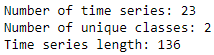
Figure 13-1. ECG five days summary

There are 23 time series, 2 unique classes, and each time series has a length of 136.

Figure 13-2 shows a few examples of each class; now we know what these ECG readings look like.

# Examples of Class 1.0
for i in range(0,10):
    if data_train[i,0]==1.0:
        print("Plot ",i," Class ",data_train[i,0])
        plt.plot(data_train[i])
        plt.show()

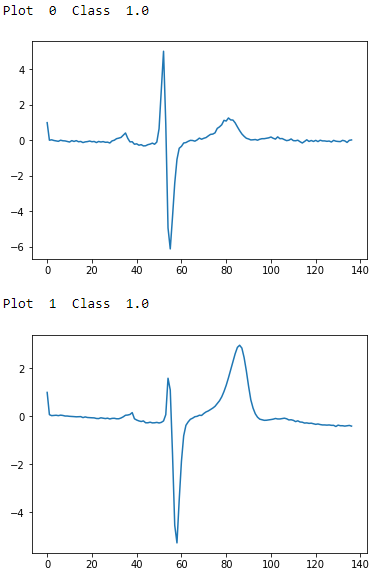
Figure 13-2. ECG five days class 1.0 - first two examples

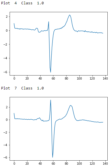
Figure 13-3. ECG five days class 1.0 - second two examples

# Examples of Class 2.0
for i in range(0,10):
    if data_train[i,0]==2.0:
        print("Plot ",i," Class ",data_train[i,0])
        plt.plot(data_train[i])
        plt.show()

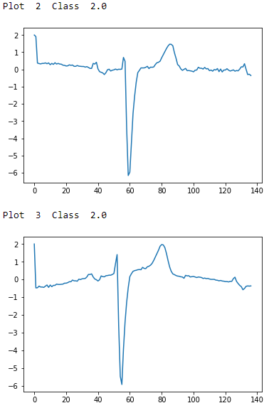
Figure 13-4. ECG five days class 2.0 - first two examples

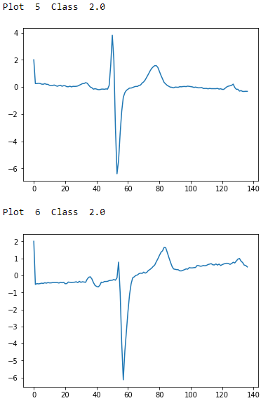
Figure 13-5. ECG five days class 2.0 - second two examples

To the naked, untrained eye, the examples from class 1.0 and class 2.0 seem indistinguisable, but these observations have been annotated by domain experts. The plots are noisy with distortions of the variety described earlier. There are differences in amplitude, period, phase shift, and vertical shift that make classification a challenge.

Let’s prepare the data for the k-Shape algorithm. We will normalize the data to have a mean of zero and standard deviation of one.

# Prepare the data - Scale
X_train = TimeSeriesScalerMeanVariance(mu=0., std=1.).fit_transform(X_train)
X_test = TimeSeriesScalerMeanVariance(mu=0., std=1.).fit_transform(X_test)

Training and Evaluation

Next, we will call the k-Shape algorithm and set the number of clusters as 2, the max iterations to perform as one hundred, and the number of rounds of training as one hundred.²

# Train using k-Shape
ks = KShape(n_clusters=2, max_iter=100, n_init=100,verbose=0)
ks.fit(X_train)

To measure the goodness of the time series clustering, we will use the adjusted Rand index, a measure of the similarity between two data clusterings adjusted for the chance grouping of elements. This is related to the accuracy measure.³

Intuitively, the Rand index measures the number of agreements in cluster assignments between the predicted clusterings and the true clusterings. If the model has an adjusted Rand index with a value close to 0.0, it is purely randomly assigning clusters; if the model has an adjusted Rand index with a value close to 1.0, the predicted clusterings match the true clusterings exactly.

We will use the Scikit-learn implementation of the adjusted Rand index, called the adjusted_rand_score.

Let’s generate clustering predictions and then calculate the adjusted Rand index.

# Make predictions and calculate adjusted Rand index
preds = ks.predict(X_train)
ars = adjusted_rand_score(data_train[:,0],preds)
print("Adjusted Rand Index:", ars)

Based on this run, the adjusted Rand index is 0.668 (see Figure 13-6). If you perform this training and prediction several times, you will notice the adjusted Rand index will vary a bit but remains well above 0.0 at all times.

Figure 13-6. ECG five days adjusted rand index on train set

Let’s predict on the test set and calculate the adjusted Rand index for it.

# Make predictions on test set and calculate adjusted Rand index
preds_test = ks.predict(X_test)
ars = adjusted_rand_score(data_test[:,0],preds_test)
print("Adjusted Rand Index on Test Set:", ars)

The adjusted Rand index is considerably lower on the test set, barely above 0 (see Figure 13-7). The cluster predictions are nearly chance assignments - the time series are being grouped based on similarity with little success.

Figure 13-7. ECG five days adjusted rand index on test set

If we had a much larger training set to train our k-Shape-based time series clustering model, we would expectbetter performance on the test set.

Data Preparation

We will load in the datasets and make our own train and test split, with 80% of the five thousand readings in the custom train set and the remaining 20% in the custom test set. With this much larger training set, we should be able to develop a time series clustering model that has much better performance, both on the train set and, most importantly, on the test set.

# Load the datasets
current_path = os.getcwd()
file = '\\datasets\\ucr_time_series_data\\'
data_train = np.loadtxt(current_path+file+
                        "ECG5000/ECG5000_TRAIN",
                        delimiter=",")

data_test = np.loadtxt(current_path+file+
                       "ECG5000/ECG5000_TEST",
                       delimiter=",")

data_joined = np.concatenate((data_train,data_test),axis=0)
data_train, data_test = train_test_split(data_joined,
                                    test_size=0.20, random_state=2019)

X_train = to_time_series_dataset(data_train[:, 1:])
y_train = data_train[:, 0].astype(np.int)
X_test = to_time_series_dataset(data_test[:, 1:])
y_test = data_test[:, 0].astype(np.int)

Let’s explore this dataset.

# Summary statistics
print("Number of time series:", len(data_train))
print("Number of unique classes:", len(np.unique(data_train[:,0])))
print("Time series length:", len(data_train[0,1:]))

Figure 13-8 displays the basic summary statistics. There are four thousand readings in the training set, which are grouped into five distinct classes, and each time series has a length of 140.

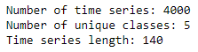
Figure 13-8. ECG 5000 summary

Let’s also consider how many of the readings belong to each of these classes.

# Calculate number of readings per class
print("Number of time series in class 1.0:",
      len(data_train[data_train[:,0]==1.0]))
print("Number of time series in class 2.0:",
      len(data_train[data_train[:,0]==2.0]))
print("Number of time series in class 3.0:",
      len(data_train[data_train[:,0]==3.0]))
print("Number of time series in class 4.0:",
      len(data_train[data_train[:,0]==4.0]))
print("Number of time series in class 5.0:",
      len(data_train[data_train[:,0]==5.0]))

The distribution is shown in Figure 13-9. Most of the readings fall in class 1, followed by class 2. Significantly fewer readings belong to clases 3, 4, and 5.

Let’s take the average time series reading from each class to get a better sense of how the various classes look.

# Display readings from each class
for j in np.unique(data_train[:,0]):
    dataPlot = data_train[data_train[:,0]==j]
    cnt = len(dataPlot)
    dataPlot = dataPlot[:,1:].mean(axis=0)
    print(" Class ",j," Count ",cnt)
    plt.plot(dataPlot)
    plt.show()

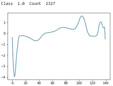
Figure 13-9. ECG 5000 class 1.0

Class 1 has a sharp trough followed by a sharp peak and stabilization. This is the most common type of reading.

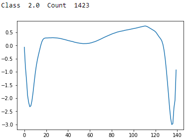
Figure 13-10. ECG 5000 class 2.0

Class 2 has a sharp trough followed by a recovery and then an even sharper and lower trough with a partial recovery. This is the second most common type of reading.

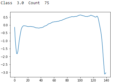
Figure 13-11. ECG 5000 class 3.0

Class 3 has a sharp trough followed by a recovery and then an even sharper and lower trough with no recovery. There are few examples of these in the dataset.

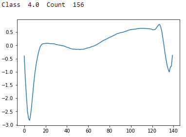
Figure 13-12. ECG 5000 class 4.0

Class 4 has a sharp trough followed by a recovery and then a shallow trough and stabilization. There are few examples of these in the dataset.

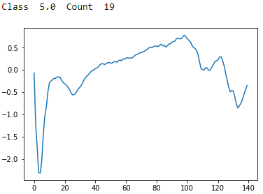
Figure 13-13. ECG 5000 class 5.0

Class 5 has a sharp trough followed by an uneven recovery, a peak, and then an unsteady decline to a shallow trough. There are very few examples of these in the dataset.

Training and Evaluation

As before, let’s normalize the data to have a mean of zero and standard deviation of one. Then, we will fit the k-shape algorithm, setting the number of clusters to five this time. Everything else remains the same.

# Prepare data - Scale
X_train = TimeSeriesScalerMeanVariance(mu=0., std=1.).fit_transform(X_train)
X_test = TimeSeriesScalerMeanVariance(mu=0., std=1.).fit_transform(X_test)

# Train using k-Shape
ks = KShape(n_clusters=5, max_iter=100, n_init=10,verbose=1,random_state=2019)
ks.fit(X_train)

Let’s evaluate the results on the training set.

# Predict on train set and calculate adjusted Rand index
preds = ks.predict(X_train)
ars = adjusted_rand_score(data_train[:,0],preds)
print("Adjusted Rand Index on Training Set:", ars)

Figure 13-14 shows the adjusted Rand index on the training set. It is considerably stronger at 0.75.

Figure 13-14. ECG 5000 adjusted rand index on training set

Let’s evaluate the results on the test set, too.

# Predict on test set and calculate adjusted Rand index
preds_test = ks.predict(X_test)
ars = adjusted_rand_score(data_test[:,0],preds_test)
print("Adjusted Rand Index on Test Set:", ars)

The adjusted Rand index on the test set is much higher, too (see Figure 13-15). It is 0.72.

Figure 13-15. ECG 5000 adjusted rand index on test set

By increasing the training set to four thousand time series (from 23), we have a considerably better-performing time series clustering model.

Let’s explore the predicted clusters some more to see just how homogenous they are. For each predicted cluster, we will evaluate the distribution of true labels. If the clusters are well-defined and homogenous, most of the readings in each cluster should have the same true label.

# Evaluate goodness of the clusters
preds_test = preds_test.reshape(1000,1)
preds_test = np.hstack((preds_test,data_test[:,0].reshape(1000,1)))
preds_test = pd.DataFrame(data=preds_test)
preds_test = preds_test.rename(columns={0: 'prediction', 1: 'actual'})

counter = 0
for i in np.sort(preds_test.prediction.unique()):
    print("Predicted Cluster ", i)
    print(preds_test.actual[preds_test.prediction==i].value_counts())
    print()
    cnt = preds_test.actual[preds_test.prediction==i] \
                        .value_counts().iloc[1:].sum()
    counter = counter + cnt
print("Count of Non-Primary Points: ", counter)

Figure 13-16 displays the homogeneity of the clusters.

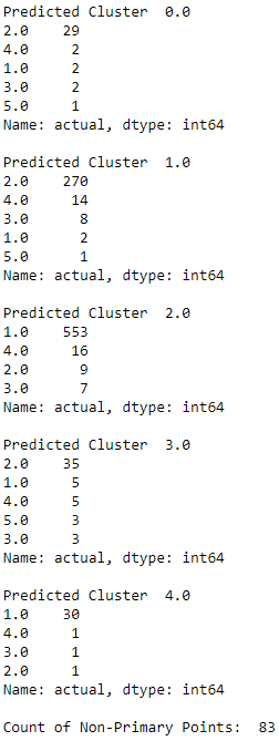
Figure 13-16. ECG 5000 k-shape predicted cluster analysis

The majority of the readings within each predicted cluster belong to just one true label class. This highlights just how well defined and homogenous the k-Shape-derived clusters are.

Full Run with k-Shape

The first experiment uses k-Shape.

# k-Shape Experiment
kShapeDF = pd.DataFrame(data=[],index=[v for v in d],
                        columns=["Train ARS","Test ARS"])

# Train and Evaluate k-Shape
class ElapsedTimer(object):
    def __init__(self):
        self.start_time = time.time()
    def elapsed(self,sec):
        if sec < 60:
            return str(sec) + " sec"
        elif sec < (60 * 60):
            return str(sec / 60) + " min"
        else:
            return str(sec / (60 * 60)) + " hr"
    def elapsed_time(self):
        print("Elapsed: %s " % self.elapsed(time.time() - self.start_time))
        return (time.time() - self.start_time)

timer = ElapsedTimer()
cnt = 0
for i in d:
    cnt += 1
    print("Dataset ", cnt)
    newpath = mypath+"\\"+i+"\\"
    onlyfiles = [f for f in listdir(newpath) if isfile(join(newpath, f))]
    j = onlyfiles[0]
    k = onlyfiles[1]
    data_train = np.loadtxt(newpath+j, delimiter=",")
    data_test = np.loadtxt(newpath+k, delimiter=",")

    data_joined = np.concatenate((data_train,data_test),axis=0)
    data_train, data_test = train_test_split(data_joined,
                                        test_size=0.20, random_state=2019)

    X_train = to_time_series_dataset(data_train[:, 1:])
    y_train = data_train[:, 0].astype(np.int)
    X_test = to_time_series_dataset(data_test[:, 1:])
    y_test = data_test[:, 0].astype(np.int)

    X_train = TimeSeriesScalerMeanVariance(mu=0., std=1.) \
                                .fit_transform(X_train)
    X_test = TimeSeriesScalerMeanVariance(mu=0., std=1.) \
                                .fit_transform(X_test)

    classes = len(np.unique(data_train[:,0]))
    ks = KShape(n_clusters=classes, max_iter=10, n_init=3,verbose=0)
    ks.fit(X_train)

    print(i)
    preds = ks.predict(X_train)
    ars = adjusted_rand_score(data_train[:,0],preds)
    print("Adjusted Rand Index on Training Set:", ars)
    kShapeDF.loc[i,"Train ARS"] = ars

    preds_test = ks.predict(X_test)
    ars = adjusted_rand_score(data_test[:,0],preds_test)
    print("Adjusted Rand Index on Test Set:", ars)
    kShapeDF.loc[i,"Test ARS"] = ars

kShapeTime = timer.elapsed_time()

It takes approximately an hour to run the k-Shape algorithm. We’ve stored the adjusted Rand indices and will use these to compare k-Shape with k-Means and hdbscan soon.

Full Run with k-Means

Next up is k-Means.

# k-Means Experiment - FULL RUN
# Create dataframe
kMeansDF = pd.DataFrame(data=[],index=[v for v in d], \
                        columns=["Train ARS","Test ARS"])

# Train and Evaluate k-Means
timer = ElapsedTimer()
cnt = 0
for i in d:
    cnt += 1
    print("Dataset ", cnt)
    newpath = mypath+"\\"+i+"\\"
    onlyfiles = [f for f in listdir(newpath) if isfile(join(newpath, f))]
    j = onlyfiles[0]
    k = onlyfiles[1]
    data_train = np.loadtxt(newpath+j, delimiter=",")
    data_test = np.loadtxt(newpath+k, delimiter=",")

    data_joined = np.concatenate((data_train,data_test),axis=0)
    data_train, data_test = train_test_split(data_joined, \
                                        test_size=0.20, random_state=2019)

    X_train = to_time_series_dataset(data_train[:, 1:])
    y_train = data_train[:, 0].astype(np.int)
    X_test = to_time_series_dataset(data_test[:, 1:])
    y_test = data_test[:, 0].astype(np.int)

    X_train = TimeSeriesScalerMeanVariance(mu=0., std=1.) \
                                    .fit_transform(X_train)
    X_test = TimeSeriesScalerMeanVariance(mu=0., std=1.) \
                                    .fit_transform(X_test)

    classes = len(np.unique(data_train[:,0]))
    km = TimeSeriesKMeans(n_clusters=5, max_iter=10, n_init=10, \
                          metric="euclidean", verbose=0, random_state=2019)
    km.fit(X_train)

    print(i)
    preds = km.predict(X_train)
    ars = adjusted_rand_score(data_train[:,0],preds)
    print("Adjusted Rand Index on Training Set:", ars)
    kMeansDF.loc[i,"Train ARS"] = ars

    preds_test = km.predict(X_test)
    ars = adjusted_rand_score(data_test[:,0],preds_test)
    print("Adjusted Rand Index on Test Set:", ars)
    kMeansDF.loc[i,"Test ARS"] = ars

kMeansTime = timer.elapsed_time()

It takes less than five minutes for k-Means to run through all 85 datasets.

Full Run with HDBSCAN

Finally, we have hdbscan.

# HDBSCAN Experiment - FULL RUN
# Create dataframe
hdbscanDF = pd.DataFrame(data=[],index=[v for v in d], \
                         columns=["Train ARS","Test ARS"])

# Train and Evaluate HDBSCAN
timer = ElapsedTimer()
cnt = 0
for i in d:
    cnt += 1
    print("Dataset ", cnt)
    newpath = mypath+"\\"+i+"\\"
    onlyfiles = [f for f in listdir(newpath) if isfile(join(newpath, f))]
    j = onlyfiles[0]
    k = onlyfiles[1]
    data_train = np.loadtxt(newpath+j, delimiter=",")
    data_test = np.loadtxt(newpath+k, delimiter=",")

    data_joined = np.concatenate((data_train,data_test),axis=0)
    data_train, data_test = train_test_split(data_joined, \
                                    test_size=0.20, random_state=2019)

    X_train = data_train[:, 1:]
    y_train = data_train[:, 0].astype(np.int)
    X_test = data_test[:, 1:]
    y_test = data_test[:, 0].astype(np.int)

    X_train = TimeSeriesScalerMeanVariance(mu=0., std=1.) \
                                    .fit_transform(X_train)
    X_test = TimeSeriesScalerMeanVariance(mu=0., std=1.)  \
                                    .fit_transform(X_test)

    classes = len(np.unique(data_train[:,0]))
    min_cluster_size = 5
    min_samples = None
    alpha = 1.0
    cluster_selection_method = 'eom'
    prediction_data = True

    hdb = hdbscan.HDBSCAN(min_cluster_size=min_cluster_size, \
                          min_samples=min_samples, alpha=alpha, \
                          cluster_selection_method= \
                              cluster_selection_method, \
                          prediction_data=prediction_data)

    print(i)
    preds = hdb.fit_predict(X_train.reshape(X_train.shape[0], \
                                            X_train.shape[1]))
    ars = adjusted_rand_score(data_train[:,0],preds)
    print("Adjusted Rand Index on Training Set:", ars)
    hdbscanDF.loc[i,"Train ARS"] = ars

    preds_test = hdbscan.prediction.approximate_predict(hdb,
                            X_test.reshape(X_test.shape[0], \
                                           X_test.shape[1]))
    ars = adjusted_rand_score(data_test[:,0],preds_test[0])
    print("Adjusted Rand Index on Test Set:", ars)
    hdbscanDF.loc[i,"Test ARS"] = ars

hdbscanTime = timer.elapsed_time()

It takes less than 10 minutes for hdbscan to run through all 85 datasets.

Compare all three time series clustering approaches

Now, let’s compare all three clustering algorithms to see which fared the best. One approach is to calculate the average adjusted Rand indices on the training and test sets, respectively, for each of the clustering algorithms.

Here are the scores for each of the algorithms (see Figures 13-21, 13-22, and 13-23).

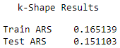
Figure 13-21. k-shape average adjusted rand index

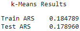
Figure 13-22. k-means average adjusted rand index

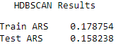
Figure 13-23. HDBSCAN average adjusted rand index

The results are fairly comparable, with k-Means having the highest Rand indices, followed closely by k-Shape and HDBSCAN.

To validate some of these findings, let’s count how many times each algorithm placed first, second, or third across all the 85 datasets.

# Count top place finishes
timeSeriesClusteringDF = pd.DataFrame(data=[],index=kShapeDF.index, \
                            columns=["kShapeTest", \
                                    "kMeansTest", \
                                    "hdbscanTest"])

timeSeriesClusteringDF.kShapeTest = kShapeDF["Test ARS"]
timeSeriesClusteringDF.kMeansTest = kMeansDF["Test ARS"]
timeSeriesClusteringDF.hdbscanTest = hdbscanDF["Test ARS"]

tscResults = timeSeriesClusteringDF.copy()

for i in range(0,len(tscResults)):
    maxValue = tscResults.iloc[i].max()
    tscResults.iloc[i][tscResults.iloc[i]==maxValue]=1
    minValue = tscResults .iloc[i].min()
    tscResults.iloc[i][tscResults.iloc[i]==minValue]=-1
    medianValue = tscResults.iloc[i].median()
    tscResults.iloc[i][tscResults.iloc[i]==medianValue]=0

# Show results
tscResultsDF = pd.DataFrame(data=np.zeros((3,3)), \
                index=["firstPlace","secondPlace","thirdPlace"], \
                columns=["kShape", "kMeans","hdbscan"])
tscResultsDF.loc["firstPlace",:] = tscResults[tscResults==1].count().values
tscResultsDF.loc["secondPlace",:] = tscResults[tscResults==0].count().values
tscResultsDF.loc["thirdPlace",:] = tscResults[tscResults==-1].count().values
tscResultsDF

k-Shape had the most first place finishes, followed by HDBSCAN. k-Means had the most second place finishes, performing neither the best but also not the worst on the majority of the datasets (see Figure 13-24).

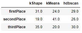
Figure 13-24. Comparison summary

Based on this comparison, it is hard to conclude that one algorithm universally trounces all the others. While k-Shape has the most first place finishes, it is considerably slower than the other two algorithms.

And, k-Means and HDBSCAN both hold their own, winning first place on a healthy number of datasets.