Restricted Boltzmann Machines

In the 2000s, Geoffrey Hinton and others began to have commercial success by using a modified version of the original unrestricted Boltzmann machines. These restricted Boltzmann machines (RBMs) have an input layer (also referred to as the visible layer) and just a single hidden layer and the connections among neurons are restricted such that neurons are connected only to the neurons in other layers but not to neurons within the same layer. In other words, there are no visibile-visible connections and no hidden-hidden connections.¹

Geoffrey Hinton also demonstrated that such simple RBMs could be stacked on top of each other such that the output of the hidden layer of one RBM can be fed into the input layer of another RBM. This sort of RBM stacking could be repeated many times to learn progressively more nuanced hidden representations of the original data.

This network of many RBMs can be viewed as one deep, multi-layered neural network model - and thus the field of deep learning took off, starting in 2006.

Note that RBMs use a stochastic approach to learn the underlying structure of data, whereas autoencoders, for example, use a deterministic approach.

Collaborative Filtering

Content-based filtering is not commonly used because it is a rather difficult task to learn the distinct properties of items - this level of understanding is very challenging for artificial machines to achieve currently.

It is much easier to collect and analyze a large amount of information on users’ behaviors and preferences and make predictions based on this. Therefore, collaborative filtering is much more widely used and is the type of recommender system we will focus on.

Collaborative filtering requires no knowledge of the underlying items themselves. Rather, collaborative filtering assumes that users that agreed in the past will agree in the future and that user preferences remain stable over time. By modeling how similar users are to other users, collaborative filtering can make pretty powerful recommendations.

Moreover, collaborative filtering does not have to rely on explicit data, i.e. ratings that users provide. Rather, it can work with implicit data such as how long or how often a user views or clicks on a particular item. Netflix, for example, used to ask users to rate movies but now uses implicit user behavior to make inferences about user likes and dislikes.

However, collaborative filtering has its challenges. First, it requires a lot of user data to make good recommendations. Second, it is a very computationally demanding task. Third, the datasets are generally very sparse since users will have exhibited preferences for only a small fraction of all the items in the universe of possible items.

Assuming we have enough data, there are techniques to handle the sparsity of the data and efficiently solve the problem, which we will cover in this chapter.

The Netflix Prize

In 2006, Netflix sponsored a three-year-long competition to improve its movie recommender system. The company offered a grand prize of one million dollars to the team that could improve the accuracy of its existing recommender system by at least 10%. It also released a dataset of over 100 million movie ratings. In September 2009, BellKor’s Pramatic Chaos team won the prize, using an ensemble of many different algorithic approaches.

Such a high profile competition with a rich dataset and meaningful prize energized the machine learning community and led to substantial progress in recommender system research, which paved the way for better recommender systems in industry over the past several years.

In this chapter, we will use a similar movie rating dataset to build our own recommender system using RBMs.

Data Preparation

As before, let’s load in the necessary libraries.

'''Main'''
import numpy as np
import pandas as pd
import os, time, re
import pickle, gzip, datetime

'''Data Viz'''
import matplotlib.pyplot as plt
import seaborn as sns
color = sns.color_palette()
import matplotlib as mpl

%matplotlib inline

'''Data Prep and Model Evaluation'''
from sklearn import preprocessing as pp
from sklearn.model_selection import train_test_split
from sklearn.model_selection import StratifiedKFold
from sklearn.metrics import log_loss
from sklearn.metrics import precision_recall_curve, average_precision_score
from sklearn.metrics import roc_curve, auc, roc_auc_score, mean_squared_error

'''Algos'''
import lightgbm as lgb

'''TensorFlow and Keras'''
import tensorflow as tf
import keras
from keras import backend as K
from keras.models import Sequential, Model
from keras.layers import Activation, Dense, Dropout
from keras.layers import BatchNormalization, Input, Lambda
from keras import regularizers
from keras.losses import mse, binary_crossentropy

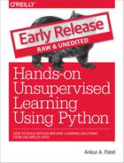
Next, we will load in the ratings dataset and convert the fields into the appropriate data types. We have just a few fields. The user ID, the movie ID, the rating provided by the user for the movie, and the timestamp of the rating provided.

# Load the data
current_path = os.getcwd()
file = '\\datasets\\movielens_data\\ratings.csv'
ratingDF = pd.read_csv(current_path + file)

# Convert fields into appropriate data types
ratingDF.userId = ratingDF.userId.astype(str).astype(int)
ratingDF.movieId = ratingDF.movieId.astype(str).astype(int)
ratingDF.rating = ratingDF.rating.astype(str).astype(float)
ratingDF.timestamp = ratingDF.timestamp.apply(lambda x: \
                datetime.utcfromtimestamp(x).strftime('%Y-%m-%d %H:%M:%S'))

Figure 10-1 shows a partial view of the data.

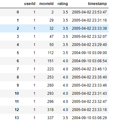
Figure 10-1. MovieLens ratings data

Let’s confirm that the number of unique users, unique movies, and total ratings, and we will also calculate the average number of ratings provided by users.

n_users = ratingDF.userId.unique().shape[0]
n_movies = ratingDF.movieId.unique().shape[0]
n_ratings = len(ratingDF)
avg_ratings_per_user = n_ratings/n_users

print('Number of unique users: ', n_users)
print('Number of unique movies: ', n_movies)
print('Number of total ratings: ', n_ratings)
print('Average number of ratings per user: ', avg_ratings_per_user)

Figure 10-2 summarizes the data. The data is as we expected.

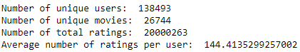
Figure 10-2. Summary stats of original data

To reduce the complexity and size of this dataset, let’s focus on the top 1000 most rated movies. This will reduce the number of ratings from _{20 million to} 12.8 million.

movieIndex = ratingDF.groupby("movieId").count().sort_values(by= \
                "rating",ascending=False)[0:1000].index
ratingDFX2 = ratingDF[ratingDF.movieId.isin(movieIndex)]
ratingDFX2.count()

We will also take a sample of 1,000 users at random and filter the dataset for just these users. This will reduce the number of ratings from ~12.8 million to just 90,213. This number is sufficient to demonstrate collaborative filtering.

userIndex = ratingDFX2.groupby("userId").count().sort_values(by= \
    "rating",ascending=False).sample(n=1000, random_state=2018).index
ratingDFX3 = ratingDFX2[ratingDFX2.userId.isin(userIndex)]
ratingDFX3.count()

Let’s also reindex movieID and userID to a range of 1 to 1000 for our reduced dataset.

movies = ratingDFX3.movieId.unique()
moviesDF = pd.DataFrame(data=movies,columns=['originalMovieId'])
moviesDF['newMovieId'] = moviesDF.index+1

users = ratingDFX3.userId.unique()
usersDF = pd.DataFrame(data=users,columns=['originalUserId'])
usersDF['newUserId'] = usersDF.index+1

ratingDFX3 = ratingDFX3.merge(moviesDF,left_on='movieId', \
                              right_on='originalMovieId')
ratingDFX3.drop(labels='originalMovieId', axis=1, inplace=True)

ratingDFX3 = ratingDFX3.merge(usersDF,left_on='userId', \
                              right_on='originalUserId')
ratingDFX3.drop(labels='originalUserId', axis=1, inplace=True)

Let’s calculate the number of unique users, unique movies, total ratings, and average number of ratings per user for our reduced dataset.

n_users = ratingDFX3.userId.unique().shape[0]
n_movies = ratingDFX3.movieId.unique().shape[0]
n_ratings = len(ratingDFX3)
avg_ratings_per_user = n_ratings/n_users

print('Number of unique users: ', n_users)
print('Number of unique movies: ', n_movies)
print('Number of total ratings: ', n_ratings)
print('Average number of ratings per user: ', avg_ratings_per_user)

Figure 10-3 displays the results, which are as expected.

Figure 10-3. Summary stats of new data

Let’s generate a test set and a validation set from this reduced dataset such that each holdout set is 5% of the reduced dataset.

X_train, X_test = train_test_split(ratingDFX3,
 test_size=0.10, shuffle=True, random_state=2018)

X_validation, X_test = train_test_split(X_test,
 test_size=0.50, shuffle=True, random_state=2018)

Figure 10-4 shows the sizes of the train, validation, and test sets.

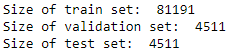
Figure 10-4. Size of train, validation, and test sets

Define the Cost Function: Mean Squared Error

Now we are ready to work with the data.

First, let’s create a matrix m x n, where m are the users and n are the movies. This will be a sparsely populated matrix because users rate only a fraction of the movies. Specifically, for this one thousand users x one thousand movies matrix, we have only 81,191 ratings in the training set. In other words, nearly 92% of the matrix will be zeros.

# Generate ratings matrix for train
ratings_train = np.zeros((n_users, n_movies))
for row in X_train.itertuples():
    ratings_train[row[6]-1, row[5]-1] = row[3]

# Calculate sparsity of the train ratings matrix
sparsity = float(len(ratings_train.nonzero()[0]))
sparsity /= (ratings_train.shape[0] * ratings_train.shape[1])
sparsity *= 100
print('Sparsity: {:4.2f}%'.format(sparsity))

We will generate similar matrices for the validation set and the test set, which will be even sparser, of course.

# Generate ratings matrix for validation
ratings_validation = np.zeros((n_users, n_movies))
for row in X_validation.itertuples():
    ratings_validation[row[6]-1, row[5]-1] = row[3]

# Generate ratings matrix for test
ratings_test = np.zeros((n_users, n_movies))
for row in X_test.itertuples():
    ratings_test[row[6]-1, row[5]-1] = row[3]

Before we build recommender systems, let’s define the cost function that we will use to judge the goodness of our model. We will use mean_squared_error (MSE), one of the simplest cost functions in machine learning. MSE measures the averaged squared error between the predicted values and the actual values.

To calculate the mean squared error, we need two vectors of size [n,1], where n are the number of ratings we are predicting - 4,511 for the validation set. One vector has the actual ratings, and the other vector has the predictions.

Let’s first flatten the sparse matrix with the ratings for the validation set. This will be the vector of actual ratings.

actual_validation = ratings_validation[ratings_validation.nonzero()].flatten()

Perform Baseline Experiments

As a baseline, let’s predict an average rating of 3.5 for the validation set and calculate the mean squared error.

pred_validation = np.zeros((len(X_validation),1))
pred_validation[pred_validation==0] = 3.5
pred_validation

mean_squared_error(pred_validation, actual_validation)

As a baseline, let’s predict an average rating of 3.5 for the validation set and calculate the mean squared error.

The MSE of this very naive prediction is 1.05 (see Figure 10-5). This is our baseline.

Figure 10-5. Mean squared error of naive prediction

Let’s see if we can improve results by predicting a user’s rating for a given movie based on that user’s average rating for all other movies.

ratings_validation_prediction = np.zeros((n_users, n_movies))
i = 0
for row in ratings_train:
    ratings_validation_prediction[i][ratings_validation_prediction[i]==0] \
        = np.mean(row[row>0])
    i += 1

pred_validation = ratings_validation_prediction \
    [ratings_validation.nonzero()].flatten()
user_average = mean_squared_error(pred_validation, actual_validation)
print('Mean squared error using user average:', user_average)

The MSE improves to 0.909 (see Figure 10-6).

Figure 10-6. Mean squared error using user average

Now, let’s predict a user’s rating for a given movie based on the average rating all other users have given that movie.

ratings_validation_prediction = np.zeros((n_users, n_movies)).T
i = 0
for row in ratings_train.T:
    ratings_validation_prediction[i][ratings_validation_prediction[i]==0] \
        = np.mean(row[row>0])
    i += 1

ratings_validation_prediction = ratings_validation_prediction.T
pred_validation = ratings_validation_prediction \
    [ratings_validation.nonzero()].flatten()
movie_average = mean_squared_error(pred_validation, actual_validation)
print('Mean squared error using movie average:', movie_average)

The MSE of this approach is 0.914, similar to that using user average (see Figure 10-7).

Figure 10-7. Mean squared error using movie average

One Latent Factor

Let’s start with the simplest form of matrix factorization - with just one latent factor.

We will use Keras to perform matrix factorization.

First, we need to define the graph. The input is the one-dimensional vector of users for the user embedding and the one-dimensional vector of movies for the movie embedding.

We will embed these input vectors into a latent space of one and then flatten them.

To generate the output vector product, we will take the dot product of the movie vector and user vector.

We will use the Adam optimizer to minimize our cost fuction, which is defined as the mean_squared_error.

n_latent_factors = 1

user_input = Input(shape=[1], name='user')
user_embedding = Embedding(input_dim=n_users + 1, output_dim=n_latent_factors,
 name='user_embedding')(user_input)
user_vec = Flatten(name='flatten_users')(user_embedding)

movie_input = Input(shape=[1], name='movie')
movie_embedding = Embedding(input_dim=n_movies + 1, output_dim=n_latent_factors,
 name='movie_embedding')(movie_input)
movie_vec = Flatten(name='flatten_movies')(movie_embedding)

product = dot([movie_vec, user_vec], axes=1)
model = Model(inputs=[user_input, movie_input], outputs=product)
model.compile('adam', 'mean_squared_error')

Let’s train the model by feeding in the user and movie vectors from the training dataset. We will also evaluate the model on the validation set while we train. The mean squared error will be calculated against the actual ratings we have.

We will train for one hundred epochs and store the history of the training and validation results. Let’s also plot the results.

history = model.fit(x=[X_train.newUserId, X_train.newMovieId], \
                    y=X_train.rating, epochs=100, \
                    validation_data=([X_validation.newUserId, \
                    X_validation.newMovieId], X_validation.rating), \
                    verbose=1)

pd.Series(history.history['val_loss'][10:]).plot(logy=False)
plt.xlabel("Epoch")
plt.ylabel("Validation Error")
print('Minimum MSE: ', min(history.history['val_loss']))

Figure 10-8 shows the results.

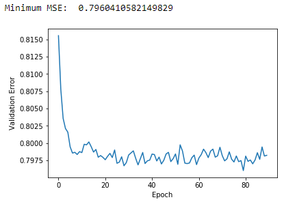
Figure 10-8. Plot of validation MSE using MF and one latent factor

The minimum MSE using matrix factorization and one latent factor is 0.796. This is a better MSE than our user average and movie average approaches earlier.

Let’s see if we can do even better by increasing the number of latent factors (i.e., the capacity of the model).

Three Latent Factors

Figure 10-9 displays the results using three latent factors.

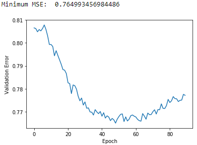
Figure 10-9. Plot of validation MSE using MF and three latent factors

The minimum MSE is 0.765, which is better than the one using one latent factor and the best yet.

Five Latent Factors

Let’s now build a matrix factorization model using five latent factors (see Figure 10-10 for the results).

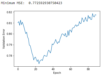
Figure 10-10. Plot of validation MSE using MF and five latent factors

The minimum MSE fails to improve, and there are clear signs of overfitting after the first 25 epochs or so. The validation error troughs and then begins to increase. Adding more capacity to the matrix factorization model will not help much more.

RBM Neural Network Architecture

For our movie-recommender system, we have an m x n matrix with m users and n movies. To train the RBM, we pass along a batch of k users with their n movie ratings into the neural network and train for a certain number of epochs.

Each input x that is passed into the neural network represents a single user’s rating preferences for all n movies, where n is one thousand in our example. Therefore, the visible layer has n nodes, one for each movie.

We can specify the number of nodes in the hidden layer, which will generally be fewer than the nodes in the visible layer to force the hidden layer to learn the most salient aspects of the original input as efficiently as possible.

Each input v0 is multiplied by its respective weight W, which are learned by the connections from the visible layer to the hidden layer. Then we add a bias vector at the hidden layer called hb. The bias ensures that at least some of the neurons fire. This W*v0+hb result is passed through an activation function.

After this, we will take a sample of the outputs generated via a sampling process known as Gibbs sampling. In other words, the activation of the hidden layer results in final outputs that are generated stochastically. This level of randomness helps build a better-performing and more robust generative model.

Next, the output after Gibbs sampling - known as h0 - is passed back through the neural network in the opposite direction in what is called a backward pass. In the backward pass, the activations in the forward pass after Gibbs sampling are fed into the hidden layer and multiplied by the same weights W as before. We then add a new bias vector at the visible layer called vb.

This W_h0+vb is passed through an activation function, and then we perform Gibbs sampling. The output of this is v1, which is then passed as the new input into the visible layer and through the neural network as another forward pass.

The RBM goes through a series of forward and backward passes like this to learn the optimal weights as it attempts to build a robust generative model.

RBMs are the first type of generative learning model that we have explored. By performing Gibbs sampling and re-training weights via forward and backward passes, RBMs are trying to learn the probability distribution of the original input.

Specifically, RBMs minimize the Kullback-Leibler Divergence, which measures how one probability distribution is different from another; in this case, RBMs are minimizing the probability distribution of the original input from the probability distribution of the reconstructed data.

By iteratively re-adjusting the weights in the neural net, the RBM learns to approximate the original data as best as possible.

With this newly learned probability distribution, RBMs are able to make predictions about never before seen data. In this case, the RBM we design will attempt to predict ratings for movies that the user has never seen based on the user’s similarity to other users and the ratings those movies have received by the other users.

Build the Components of the RBM Class

First, we will initialize the class with a few parameters; these are the input size of the RBM, the output size, the learning rate, the number of epochs to train for, and the batch size during the training process.

We will also create zero matrices for the weight matrix, the hidden bias vector, and the visible bias vector.

# Define RBM class
class RBM(object):

    def __init__(self, input_size, output_size,
                 learning_rate, epochs, batchsize):
        # Define hyperparameters
        self._input_size = input_size
        self._output_size = output_size
        self.learning_rate = learning_rate
        self.epochs = epochs
        self.batchsize = batchsize

        # Initialize weights and biases using zero matrices
        self.w = np.zeros([input_size, output_size], "float")
        self.hb = np.zeros([output_size], "float")
        self.vb = np.zeros([input_size], "float")

Next, let’s define functions for the forward pass, the backward pass, and the sampling of data during each of these passes back and forth.

Here is the forward pass, where h is the hidden layer and v is the visible layer.

def prob_h_given_v(self, visible, w, hb):
    return tf.nn.sigmoid(tf.matmul(visible, w) + hb)

Here is the backward pass.

def prob_v_given_h(self, hidden, w, vb):
    return tf.nn.sigmoid(tf.matmul(hidden, tf.transpose(w)) + vb)

Here is the sampling function.

def sample_prob(self, probs):
    return tf.nn.relu(tf.sign(probs - tf.random_uniform(tf.shape(probs))))

Now, we need a function that performs that training. Since we are using TensorFlow, we first need to create placeholders for the TensorFlow graph, which we will use when we feed data into the TensorFlow session.

We will have placeholders for the weights matrix, the hidden bias vector, and the visible bias vector.

We will also need to initialize the values for these three using zeros. And, we will need one set to hold the current values and one set to hold the previous values.

_w = tf.placeholder("float", [self._input_size, self._output_size])
_hb = tf.placeholder("float", [self._output_size])
_vb = tf.placeholder("float", [self._input_size])

prv_w = np.zeros([self._input_size, self._output_size], "float")
prv_hb = np.zeros([self._output_size], "float")
prv_vb = np.zeros([self._input_size], "float")

cur_w = np.zeros([self._input_size, self._output_size], "float")
cur_hb = np.zeros([self._output_size], "float")
cur_vb = np.zeros([self._input_size], "float")

Likewise, we need a placeholder for the visible layer. The hidden layer is derived from matrix multiplication of the visible layer and the weights matrix and the matrix addition of the hidden bias vector.

v0 = tf.placeholder("float", [None, self._input_size])
h0 = self.sample_prob(self.prob_h_given_v(v0, _w, _hb))

During the backward pass, we take the hidden layer output, multiply it with the transpose of the weights matrix used during the forward pass and add the visible bias vector. Note that the weights matrix is the same weights matrix during both the forward and the backward pass.

And, then, we perform the forward pass again.

v1 = self.sample_prob(self.prob_v_given_h(h0, _w, _vb))
h1 = self.prob_h_given_v(v1, _w, _hb)

To update the weights, we perform constrastive divergence.²

We also define the error as mean squared error.

positive_grad = tf.matmul(tf.transpose(v0), h0)
negative_grad = tf.matmul(tf.transpose(v1), h1)

update_w = _w + self.learning_rate * \
    (positive_grad - negative_grad) / tf.to_float(tf.shape(v0)[0])
update_vb = _vb +  self.learning_rate * tf.reduce_mean(v0 - v1, 0)
update_hb = _hb +  self.learning_rate * tf.reduce_mean(h0 - h1, 0)

err = tf.reduce_mean(tf.square(v0 - v1))

With this, we are ready to initialize the TensorFlow session with the variables we have just defined.

Once we call sess.run, we can feed in batches of data to begin the training. During the training, forward and backward passes will be made, and the RBM will update weights based on how the generated data compares to the original input. We will print the reconstruction error from each epoch.

with tf.Session() as sess:
 sess.run(tf.global_variables_initializer())

 for epoch in range(self.epochs):
     for start, end in zip(range(0, len(X),
      self.batchsize),range(self.batchsize,len(X), self.batchsize)):
         batch = X[start:end]
         cur_w = sess.run(update_w, feed_dict={v0: batch,
          _w: prv_w, _hb: prv_hb, _vb: prv_vb})
         cur_hb = sess.run(update_hb, feed_dict={v0: batch,
          _w: prv_w, _hb: prv_hb, _vb: prv_vb})
         cur_vb = sess.run(update_vb, feed_dict={v0: batch,
          _w: prv_w, _hb: prv_hb, _vb: prv_vb})
         prv_w = cur_w
         prv_hb = cur_hb
         prv_vb = cur_vb
     error = sess.run(err, feed_dict={v0: X,
      _w: cur_w, _vb: cur_vb, _hb: cur_hb})
     print ('Epoch: %d' % epoch,'reconstruction error: %f' % error)
 self.w = prv_w
 self.hb = prv_hb
 self.vb = prv_vb

Train RBM Recommender System

To train the RBM, let’s create a NumPy array called inputX from ratings_train and convert these values to float32.

We will also define the RBM to take in a one thousand-dimensional input, output a one thousand-dimensional output, use a learning rate of 0.3, train for five hundred epochs, and use a batch size of two hundred. These parameters are just prelimary basic parameter choices; you should be able to find more optimal parameters with experimentation, which is encouraged.

# Begin the training cycle

# Convert inputX into float32
inputX = ratings_train
inputX = inputX.astype(np.float32)

# Define the parameters of the RBMs we will train
rbm=RBM(1000,1000,0.3,500,200)

Let’s begin training.

rbm.train(inputX)
outputX, reconstructedX, hiddenX = rbm.rbm_output(inputX)

Figure 10-11 displays the plot of the reconstruction errors.

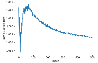
Figure 10-11. Plot of RBM errors

The error terms generally decrease the longer we train.

Now, let’s take the RBM model we developed to predict the ratings for users in the validation set (which has the same users as the training set).

# Predict ratings for validation set
inputValidation = ratings_validation
inputValidation = inputValidation.astype(np.float32)

finalOutput_validation, reconstructedOutput_validation, _ = \
    rbm.rbm_output(inputValidation)

Now, let’s convert the predictions into an array and calculate the mean squared error against the true validation ratings.

predictionsArray = reconstructedOutput_validation
pred_validation = \
    predictionsArray[ratings_validation.nonzero()].flatten()
actual_validation = \
    ratings_validation[ratings_validation.nonzero()].flatten()

rbm_prediction = mean_squared_error(pred_validation, actual_validation)
print('Mean squared error using RBM prediction:', rbm_prediction)

Figure 10-12 displays the mean squared error on the validation set.

Figure 10-12. Mean squared error of RBM on validation set

This MSE of 9.33 is a starting point and will likely improve with greater experimentation.