Table of Contents for
Hands-On Unsupervised Learning Using Python
 Hands-On Unsupervised Learning Using Python
Published by
O'Reilly Media, Inc., 2019
Hands-On Unsupervised Learning Using Python
Published by
O'Reilly Media, Inc., 2019
- Cover
- nav
- Hands-on Unsupervised Learning Using Python
- Hands-On Unsupervised Learning Using Python
- Preface
- I. Fundamentals of Unsupervised Learning
- 1. Unsupervised Learning in the Machine Learning Ecosystem
- 2. End-to-End Machine Learning Project
- II. Unsupervised Learning Using Scikit-Learn
- 3. Dimensionality Reduction
- 4. Anomaly Detection
- 5. Clustering
- 6. Group Segmentation
- III. Unsupervised Learning using TensorFlow and Keras
- 7. Autoencoders
- 8. Hands-On Autoencoder
- 9. Semi-Supervised Learning
- IV. Deep Unsupervised Learning using TensorFlow and Keras
- 10. Recommender Systems Using Restricted Boltzmann Machines
- 11. Feature Detection Using Deep Belief Networks
- 12. Generative Adversarial Networks
- 13. Time Series Clustering
- 14. Conclusion
- Index
- About the Author
Chapter 11. Feature Detection Using Deep Belief Networks
In Chapter 10, we explored restricted Boltzmann machines and used them to build a recommender system for movie ratings. In this chapter, we will stack RBMs together to build deep belief networks (DBNs). DBNs were first introduced by Geoff Hinton at the University of Toronto in 2006.
RBMs have just two layers, a visible layer and a hidden layer; in other words, RBMs are a just a shallow neural network. DBNs are made up of multiple RBMs - the hidden layer of one RBM serves as the visible layer of the next RBM. Because they involve many layers, DBNs are a deep neural network. In fact, they are the first deep unsupervised neural network we’ve introduced so far.
A shallow unsupervised neural network, such as RBMs, cannot capture structure in complex data such as images, sound, and text, but DBNs can. DBNs have been used to recognize and cluster images, video capture, sound, and text, although other deep learning methods have surpassed DBNs in performance over the past decade.
Deep Belief Networks in Detail
Like RBMs, DBNs can learn the underlying structure of the input and probabilistically reconstruct it. In other words, DBNs - like RBMs - are generative models. And, as with RBMs, the layers in DBNs have connections only between layers but not between units within each layer.
In the DBN, each layer is trained at a time, starting with the very first hidden layer, which, along with the input layer, makes up the first RBM. Once this first RBM is trained, the hidden layer of the first RBM serves as the visible layer of the next RBM and is used to trained the second hidden layer of the DBN.
This process continues until all the layers of the DBN are trained. Except for the first and final layers of the DBN, each layer in the DBN serves as both a hidden layer and a visible layer of a RBM.
The DBN is a hierarchy of representations and, like all neural networks, is a form of representation learning. Note that the DBN does not use any labels. Instead, the DBN is learning the underlying structure in the input data one layer at a time.
Labels can be used to fine-tune the last few layers of the DBN but only after the initial unsupervised learning has been done. For example, if we want the DBN to be a classifier, we would perform unsupervised learning first - a process known as pre-training - and then use the labels to fine-tune the DBN - a process known as fine-tuning.
MNIST Image Classification
Let’s build an image classifier using DBNs. We will turn to the MNIST dataset once again.
First, let’s load the necessary libraries.
'''Main'''importnumpyasnpimportpandasaspdimportos,time,reimportpickle,gzip,datetime'''Data Viz'''importmatplotlib.pyplotaspltimportseabornassnscolor=sns.color_palette()importmatplotlibasmpl%matplotlibinline'''Data Prep and Model Evaluation'''fromsklearnimportpreprocessingasppfromsklearn.model_selectionimporttrain_test_splitfromsklearn.model_selectionimportStratifiedKFoldfromsklearn.metricsimportlog_loss,accuracy_scorefromsklearn.metricsimportprecision_recall_curve,average_precision_scorefromsklearn.metricsimportroc_curve,auc,roc_auc_score,mean_squared_error'''Algos'''importlightgbmaslgb'''TensorFlow and Keras'''importtensorflowastfimportkerasfromkerasimportbackendasKfromkeras.modelsimportSequential,Modelfromkeras.layersimportActivation,Dense,Dropoutfromkeras.layersimportBatchNormalization,Input,Lambdafromkeras.layersimportEmbedding,Flatten,dotfromkerasimportregularizersfromkeras.lossesimportmse,binary_crossentropy
We will then load the data and store the data in Pandas dataframes. We will also encode the labels as one-hot vectors. This is all similar to what we did when we first introduced the MNIST dataset earlier in the book.
# Load the datasetscurrent_path=os.getcwd()file='\\datasets\\mnist_data\\mnist.pkl.gz'f=gzip.open(current_path+file,'rb')train_set,validation_set,test_set=pickle.load(f,encoding='latin1')f.close()X_train,y_train=train_set[0],train_set[1]X_validation,y_validation=validation_set[0],validation_set[1]X_test,y_test=test_set[0],test_set[1]# Create Pandas DataFrames from the datasetstrain_index=range(0,len(X_train))validation_index=range(len(X_train),len(X_train)+len(X_validation))test_index=range(len(X_train)+len(X_validation),\len(X_train)+len(X_validation)+len(X_test))X_train=pd.DataFrame(data=X_train,index=train_index)y_train=pd.Series(data=y_train,index=train_index)X_validation=pd.DataFrame(data=X_validation,index=validation_index)y_validation=pd.Series(data=y_validation,index=validation_index)X_test=pd.DataFrame(data=X_test,index=test_index)y_test=pd.Series(data=y_test,index=test_index)defview_digit(X,y,example):label=y.loc[example]image=X.loc[example,:].values.reshape([28,28])plt.title('Example:%dLabel:%d'%(example,label))plt.imshow(image,cmap=plt.get_cmap('gray'))plt.show()defone_hot(series):label_binarizer=pp.LabelBinarizer()label_binarizer.fit(range(max(series)+1))returnlabel_binarizer.transform(series)# Create one-hot vectors for the labelsy_train_oneHot=one_hot(y_train)y_validation_oneHot=one_hot(y_validation)y_test_oneHot=one_hot(y_test)
Restricted Boltzmann Machines
Next, let’s define a Restricted Boltzmann Machine (RBM) class so we can train several RBMs - which are the building blocks for DBNs - in quick succession.
Recall that RBMs have an input layer (also referred to as the visible layer) and a single hidden layer, and the connections among neurons are restricted such that neurons are connected only to the neurons in other layers but not to neurons within the same layer.
Also, recall that communication between layers happens in both direction - not just in one direction/feedforward way as in the case of autoencoders.
In a RBM, the neurons in the visible layer communicate with the hidden layer, the hidden layer generates data from the probabilistic model the RBM has learned, and then the hidden layer passes this generated information back to the visible layer.
The visible layer takes the generated data from the hidden layer, samples it, compares this to the original data, and, based on the reconstruction error between the generated data sample and the original data, sends new information to the hidden layer to repeat the process once again.
By communicating in this bi-directional way, the RBM develops a generative model such that the reconstructions from the outputs of the hidden layer are similar to the original inputs.
Build the Components of the RBM Class
Like we did in Chapter 10, let’s walk through the various components of the RBM class.
First, we will initialize the class with a few parameters; these are the input size of the RBM, the output size, the learning rate, the number of epochs to train for, and the batch size during the training process.
We will also create zero matrices for the weight matrix, the hidden bias vector, and the visible bias vector.
# Define RBM classclassRBM(object):def__init__(self,input_size,output_size,learning_rate,epochs,batchsize):# Define hyperparametersself._input_size=input_sizeself._output_size=output_sizeself.learning_rate=learning_rateself.epochs=epochsself.batchsize=batchsize# Initialize weights and biases using zero matricesself.w=np.zeros([input_size,output_size],"float")self.hb=np.zeros([output_size],"float")self.vb=np.zeros([input_size],"float")
Next, let’s define functions for the forward pass, the backward pass, and the sampling of data during each of these passes back and forth.
Here is the forward pass, where h is the hidden layer and v is the visible layer.
defprob_h_given_v(self,visible,w,hb):returntf.nn.sigmoid(tf.matmul(visible,w)+hb)
Here is the backward pass.
defprob_v_given_h(self,hidden,w,vb):returntf.nn.sigmoid(tf.matmul(hidden,tf.transpose(w))+vb)
Here is the sampling function.
defsample_prob(self,probs):returntf.nn.relu(tf.sign(probs-tf.random_uniform(tf.shape(probs))))
Now, we need a function that performs that training. Since we are using TensorFlow, we first need to create placeholders for the TensorFlow graph, which we will use when we feed data into the TensorFlow session.
We will have placeholders for the weights matrix, the hidden bias vector, and the visible bias vector.
We will also need to initialize the values for these three using zeros. And, we will need one set to hold the current values and one set to hold the previous values.
_w=tf.placeholder("float",[self._input_size,self._output_size])_hb=tf.placeholder("float",[self._output_size])_vb=tf.placeholder("float",[self._input_size])prv_w=np.zeros([self._input_size,self._output_size],"float")prv_hb=np.zeros([self._output_size],"float")prv_vb=np.zeros([self._input_size],"float")cur_w=np.zeros([self._input_size,self._output_size],"float")cur_hb=np.zeros([self._output_size],"float")cur_vb=np.zeros([self._input_size],"float")
Likewise, we need a placeholder for the visible layer. The hidden layer is derived from matrix multiplication of the visible layer and the weights matrix and the matrix addition of the hidden bias vector.
v0=tf.placeholder("float",[None,self._input_size])h0=self.sample_prob(self.prob_h_given_v(v0,_w,_hb))
During the backward pass, we take the hidden layer output, multiply it with the transpose of the weights matrix used during the forward pass and add the visible bias vector. Note that the weights matrix is the same weights matrix during both the forward and the backward pass.
And, then, we perform the forward pass again.
v1=self.sample_prob(self.prob_v_given_h(h0,_w,_vb))h1=self.prob_h_given_v(v1,_w,_hb)
To update the weights, we perform constrastive divergence, which we introduced in Chapter 10. We also define the error as mean squared error.
positive_grad=tf.matmul(tf.transpose(v0),h0)negative_grad=tf.matmul(tf.transpose(v1),h1)update_w=_w+self.learning_rate*\(positive_grad-negative_grad)/tf.to_float(tf.shape(v0)[0])update_vb=_vb+self.learning_rate*tf.reduce_mean(v0-v1,0)update_hb=_hb+self.learning_rate*tf.reduce_mean(h0-h1,0)err=tf.reduce_mean(tf.square(v0-v1))
With this, we are ready to initialize the TensorFlow session with the variables we have just defined.
Once we call sess.run, we can feed in batches of data to begin the training. During the training, forward and backward passes will be made, and the RBM will update weights based on how the generated data compares to the original input. We will print the reconstruction error from each epoch.
withtf.Session()assess:sess.run(tf.global_variables_initializer())forepochinrange(self.epochs):forstart,endinzip(range(0,len(X),self.batchsize),\range(self.batchsize,len(X),self.batchsize)):batch=X[start:end]cur_w=sess.run(update_w,\feed_dict={v0:batch,_w:prv_w,\_hb:prv_hb,_vb:prv_vb})cur_hb=sess.run(update_hb,\feed_dict={v0:batch,_w:prv_w,\_hb:prv_hb,_vb:prv_vb})cur_vb=sess.run(update_vb,\feed_dict={v0:batch,_w:prv_w,\_hb:prv_hb,_vb:prv_vb})prv_w=cur_wprv_hb=cur_hbprv_vb=cur_vberror=sess.run(err,feed_dict={v0:X,_w:cur_w,\_vb:cur_vb,_hb:cur_hb})('Epoch:%d'%epoch,'reconstruction error:%f'%error)self.w=prv_wself.hb=prv_hbself.vb=prv_vb
Generate Images Using the RBM Model
Let’s also define a function to generate new images from the generative model that the RBM has learned.
defrbm_output(self,X):input_X=tf.constant(X)_w=tf.constant(self.w)_hb=tf.constant(self.hb)_vb=tf.constant(self.vb)out=tf.nn.sigmoid(tf.matmul(input_X,_w)+_hb)hiddenGen=self.sample_prob(self.prob_h_given_v(input_X,_w,_hb))visibleGen=self.sample_prob(self.prob_v_given_h(hiddenGen,_w,_vb))withtf.Session()assess:sess.run(tf.global_variables_initializer())returnsess.run(out),sess.run(visibleGen),sess.run(hiddenGen)
We feed the original matrix of images, called X, into the function.
We create TensorFlow placeholders for the original matrix of images, the weights matrix, the hidden bias vector, and the visible bias vector.
Then, we push the input matrix to produce the output of a forward pass (out), a sample of the hidden layer (hiddenGen), and a sample of the reconstructed images generated by the model (visibleGen).
View the Intermediate Feature Detectors
Finally, let’s define a function to show the feature detectors of the hidden layer.
defshow_features(self,shape,suptitle,count=-1):maxw=np.amax(self.w.T)minw=np.amin(self.w.T)count=self._output_sizeifcount==-1orcount>\self._output_sizeelsecountncols=countifcount<14else14nrows=count//ncolsnrows=nrowsifnrows>2else3fig=plt.figure(figsize=(ncols,nrows),dpi=100)grid=Grid(fig,rect=111,nrows_ncols=(nrows,ncols),axes_pad=0.01)fori,axinenumerate(grid):x=self.w.T[i]ifi<self._input_sizeelsenp.zeros(shape)x=(x.reshape(1,-1)-minw)/maxwax.imshow(x.reshape(*shape),cmap=mpl.cm.Greys)ax.set_axis_off()fig.text(0.5,1,suptitle,fontsize=20,horizontalalignment='center')fig.tight_layout()plt.show()return
We will use this and the other functions on the MNIST dataset now.
Train the Three RBMs for the DBN
We will now use the MNIST data to train three RBMs, one at a time, such that the hidden layer of one RBM is used as the visible layer of the next RBM.
These three RBMs will make up the DBN that we are building to perform image classification.
First, let’s take the training data and store it as a NumPy array. Next, we will create a list to hold the RBMs we train, called rbm_list.
Then, we will define the hyperparameters for the three RBMs, including the input size, the output size, the learning rate, the number of epochs to train for, and the batch size for training.
All of these can be built using the RBM class we defined earlier.
For our DBN, we will use the following RBMs: the first will take the original 784-dimension input and output a 700-dimension matrix. The next RBM will use the 700-dimension matrix output of the first RBM and output a 600-dimension matrix. Finally, the last RBM we train will take the 600-dimension matrix and output a 500-dimension matrix.
We will train all three RBMs using a learning rate of 1.0, train for 100 epochs each, and use a batch size of two hundred.
# Since we are training, set input as training datainputX=np.array(X_train)# Create list to hold our RBMsrbm_list=[]# Define the parameters of the RBMs we will trainrbm_list.append(RBM(784,700,1.0,100,200))rbm_list.append(RBM(700,600,1.0,100,200))rbm_list.append(RBM(600,500,1.0,100,200))
Now, let’s train the RBMs. We will store the trained RBMs in a list called outputList.
Note that we use the rbm_output function we defined earlier to produce the output matrix - in other words, the hidden layer - for use as the input/visible layer of the subsequent RBM we train.
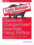
outputList=[]error_list=[]#For each RBM in our listforiinrange(0,len(rbm_list)):('RBM',i+1)#Train a new onerbm=rbm_list[i]err=rbm.train(inputX)error_list.append(err)#Return the output layeroutputX,reconstructedX,hiddenX=rbm.rbm_output(inputX)outputList.append(outputX)inputX=hiddenX
The errors of each RBM decline the longer we train (see Figures 11-1, 11-2, and 11-3). Note that the RBM error reflects how similar the reconstructed data of a given RBM is to the data fed into the visible layer of that very RBM.
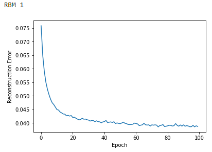
Figure 11-1. Reconstruction errors of first RBM
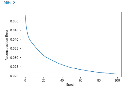
Figure 11-2. Reconstruction errors of second RBM
Figure 11-3. Reconstruction errors of third RBM
Examine Feature Detectors
Now, let’s view the learned features from each of the RBMs using the rbm.show_features function we defined earlier.
rbm_shapes=[(28,28),(25,24),(25,20)]foriinrange(0,len(rbm_list)):rbm=rbm_list[i](rbm.show_features(rbm_shapes[i],"RBM learned features from MNIST",56))
Figure 11-4 displays the learned features for the various RBMs.
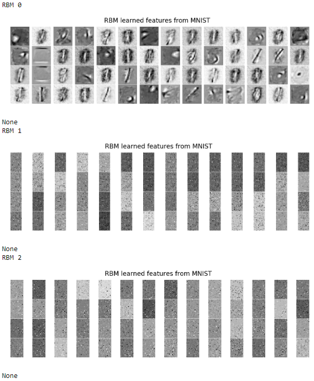
Figure 11-4. Learned features of the RBMs
As you can see, each RBM learns increasingly abstract features from the MNIST data. The features of the first RBM vaguely resemble digits, and the features of the second and the third RBMs are increasingly nuanced and less discernible. This is pretty typical of how feature detectors work on image data; the deeper layers of the neural network recognize increasingly abstract elements from the original images.
View Generated Images
Before we build the full DBN, let’s view some of the generated images from one of the RBMs we just trained.
To keep things simple, we will feed the original MNIST training matrix into the first RBM we trained, perform a forward pass and then a backward pass, and this will produce the generated images we need.
We will compare the first ten images of the MNIST dataset with the newly generated images.
inputX=np.array(X_train)rbmOne=rbm_list[0]('RBM 1')outputX_rbmOne,reconstructedX_rbmOne,hiddenX_rbmOne=rbmOne.rbm_output(inputX)reconstructedX_rbmOne=pd.DataFrame(data=reconstructedX_rbmOne,index=X_train.index)forjinrange(0,10):example=jview_digit(reconstructedX,y_train,example)view_digit(X_train,y_train,example)
Figure 11-5 shows the first image produced by the RBM compared to the first original image.
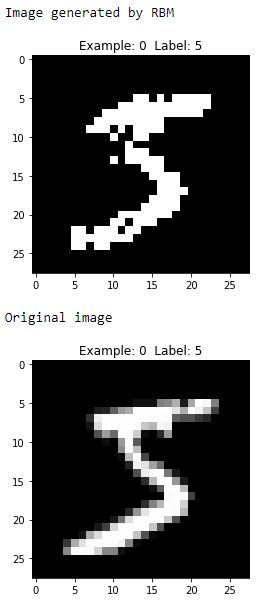
Figure 11-5. First generated image of the first RBM
As you can see, the generated image is similar to the original image — both display the digit five.
Let’s view a few more images like this to compare the RBM generated one with the original ones (see Figures 11-6 through 11-911-9).
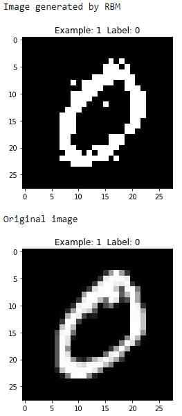
Figure 11-6. Second generated image of the first RBM
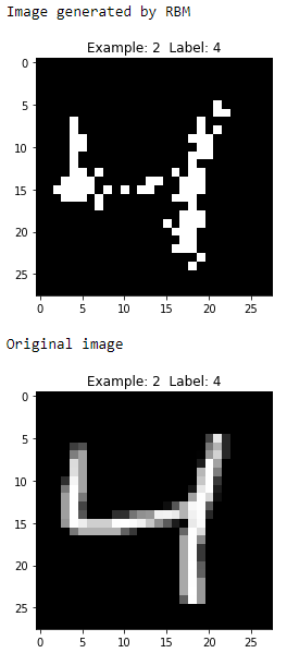
Figure 11-7. Third generated image of the first RBM
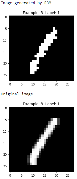
Figure 11-8. Fourth generated image of the first RBM
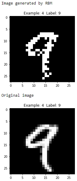
Figure 11-9. Fifth generated image of the first RBM
These digits are zero, four, one, and nine, respectively, and the generated images look reasonably similar to the original images.
The Full DBN
Now, let’s define the DBN class, which will take in the three RBMs we just trained and add a fourth RBM that performs forward and backward passes to refine the overall DBN-based generative model.
First, let’s define the hyperparameters of the class. These include the original input size, the input size of the third RBM we just trained, the final output size we would like to have from the DBN, the learning rate, the number of epochs we wish to train for, the batch size for training, and the three RBMs we just trained.
Like before, we will need to generate zero matrices for the weights, hidden bias, and visible bias.
classDBN(object):def__init__(self,original_input_size,input_size,output_size,learning_rate,epochs,batchsize,rbmOne,rbmTwo,rbmThree):# Define hyperparametersself._original_input_size=original_input_sizeself._input_size=input_sizeself._output_size=output_sizeself.learning_rate=learning_rateself.epochs=epochsself.batchsize=batchsizeself.rbmOne=rbmOneself.rbmTwo=rbmTwoself.rbmThree=rbmThreeself.w=np.zeros([input_size,output_size],"float")self.hb=np.zeros([output_size],"float")self.vb=np.zeros([input_size],"float")
Similar to before, we will define functions to perform the forward pass, the backward pass, and take samples from each.
defprob_h_given_v(self,visible,w,hb):returntf.nn.sigmoid(tf.matmul(visible,w)+hb)defprob_v_given_h(self,hidden,w,vb):returntf.nn.sigmoid(tf.matmul(hidden,tf.transpose(w))+vb)defsample_prob(self,probs):returntf.nn.relu(tf.sign(probs-tf.random_uniform(tf.shape(probs))))
For the training, we need placeholders for the weights, hidden bias, and visible bias. We also need matrices for the previous and current weights, hidden biases, and visible biases.
deftrain(self,X):_w=tf.placeholder("float",[self._input_size,self._output_size])_hb=tf.placeholder("float",[self._output_size])_vb=tf.placeholder("float",[self._input_size])prv_w=np.zeros([self._input_size,self._output_size],"float")prv_hb=np.zeros([self._output_size],"float")prv_vb=np.zeros([self._input_size],"float")cur_w=np.zeros([self._input_size,self._output_size],"float")cur_hb=np.zeros([self._output_size],"float")cur_vb=np.zeros([self._input_size],"float")
We will set a placeholder for the visible layer.
Next, we will take the initial input - the visible layer - and pass it through the three RBMs we trained earlier. This results in the output forward, which we will pass into the fourth RBM we train as part of this DBN class.
v0=tf.placeholder("float",[None,self._original_input_size])forwardOne=tf.nn.relu(tf.sign(tf.nn.sigmoid(tf.matmul(v0,\self.rbmOne.w)+self.rbmOne.hb)-tf.random_uniform(\tf.shape(tf.nn.sigmoid(tf.matmul(v0,self.rbmOne.w)+\self.rbmOne.hb)))))forwardTwo=tf.nn.relu(tf.sign(tf.nn.sigmoid(tf.matmul(forwardOne,\self.rbmTwo.w)+self.rbmTwo.hb)-tf.random_uniform(\tf.shape(tf.nn.sigmoid(tf.matmul(forwardOne,\self.rbmTwo.w)+self.rbmTwo.hb)))))forward=tf.nn.relu(tf.sign(tf.nn.sigmoid(tf.matmul(forwardTwo,\self.rbmThree.w)+self.rbmThree.hb)-\tf.random_uniform(tf.shape(tf.nn.sigmoid(tf.matmul(\forwardTwo,self.rbmThree.w)+self.rbmThree.hb)))))h0=self.sample_prob(self.prob_h_given_v(forward,_w,_hb))v1=self.sample_prob(self.prob_v_given_h(h0,_w,_vb))h1=self.prob_h_given_v(v1,_w,_hb)
We will define the contrastive divergence like we did before.
positive_grad=tf.matmul(tf.transpose(forward),h0)negative_grad=tf.matmul(tf.transpose(v1),h1)update_w=_w+self.learning_rate*(positive_grad-negative_grad)/\tf.to_float(tf.shape(forward)[0])update_vb=_vb+self.learning_rate*tf.reduce_mean(forward-v1,0)update_hb=_hb+self.learning_rate*tf.reduce_mean(h0-h1,0)
Once we generate a full forward pass through this DBN - which includes the three RBMs we trained earlier plus the latest fourth RBM - we need to send the output of the fourth RBM’s hidden layer back through the entire DBN.
This requires a backward pass through the fourth RBM as well as a backward pass through the first three.
Here is how the backward pass occurs.
We will also use mean squared error as before.
backwardOne=tf.nn.relu(tf.sign(tf.nn.sigmoid(tf.matmul(v1,\self.rbmThree.w.T)+self.rbmThree.vb)-\tf.random_uniform(tf.shape(tf.nn.sigmoid(\tf.matmul(v1,self.rbmThree.w.T)+\self.rbmThree.vb)))))backwardTwo=tf.nn.relu(tf.sign(tf.nn.sigmoid(tf.matmul(backwardOne,\self.rbmTwo.w.T)+self.rbmTwo.vb)-\tf.random_uniform(tf.shape(tf.nn.sigmoid(\tf.matmul(backwardOne,self.rbmTwo.w.T)+\self.rbmTwo.vb)))))backward=tf.nn.relu(tf.sign(tf.nn.sigmoid(tf.matmul(backwardTwo,\self.rbmOne.w.T)+self.rbmOne.vb)-\tf.random_uniform(tf.shape(tf.nn.sigmoid(\tf.matmul(backwardTwo,self.rbmOne.w.T)+\self.rbmOne.vb)))))err=tf.reduce_mean(tf.square(v0-backward))
Here is the actual training portion of the DBN class, again very similar to the RBM one earlier.
withtf.Session()assess:sess.run(tf.global_variables_initializer())forepochinrange(self.epochs):forstart,endinzip(range(0,len(X),self.batchsize),\range(self.batchsize,len(X),self.batchsize)):batch=X[start:end]cur_w=sess.run(update_w,feed_dict={v0:batch,_w:\prv_w,_hb:prv_hb,_vb:prv_vb})cur_hb=sess.run(update_hb,feed_dict={v0:batch,_w:\prv_w,_hb:prv_hb,_vb:prv_vb})cur_vb=sess.run(update_vb,feed_dict={v0:batch,_w:\prv_w,_hb:prv_hb,_vb:prv_vb})prv_w=cur_wprv_hb=cur_hbprv_vb=cur_vberror=sess.run(err,feed_dict={v0:X,_w:cur_w,_vb:\cur_vb,_hb:cur_hb})('Epoch:%d'%epoch,'reconstruction error:%f'%error)self.w=prv_wself.hb=prv_hbself.vb=prv_vb
Let’s define functions to produce generated images from the DBN and show features. These are similar to the RBM versions earlier, but we send the data through all fourth RBMs in the DBN class instead of just through a single RBM.
defdbn_output(self,X):input_X=tf.constant(X)forwardOne=tf.nn.sigmoid(tf.matmul(input_X,self.rbmOne.w)+\self.rbmOne.hb)forwardTwo=tf.nn.sigmoid(tf.matmul(forwardOne,self.rbmTwo.w)+\self.rbmTwo.hb)forward=tf.nn.sigmoid(tf.matmul(forwardTwo,self.rbmThree.w)+\self.rbmThree.hb)_w=tf.constant(self.w)_hb=tf.constant(self.hb)_vb=tf.constant(self.vb)out=tf.nn.sigmoid(tf.matmul(forward,_w)+_hb)hiddenGen=self.sample_prob(self.prob_h_given_v(forward,_w,_hb))visibleGen=self.sample_prob(self.prob_v_given_h(hiddenGen,_w,_vb))backwardTwo=tf.nn.sigmoid(tf.matmul(visibleGen,self.rbmThree.w.T)+\self.rbmThree.vb)backwardOne=tf.nn.sigmoid(tf.matmul(backwardTwo,self.rbmTwo.w.T)+\self.rbmTwo.vb)backward=tf.nn.sigmoid(tf.matmul(backwardOne,self.rbmOne.w.T)+\self.rbmOne.vb)withtf.Session()assess:sess.run(tf.global_variables_initializer())returnsess.run(out),sess.run(backward)
defshow_features(self,shape,suptitle,count=-1):maxw=np.amax(self.w.T)minw=np.amin(self.w.T)count=self._output_sizeifcount==-1orcount>\self._output_sizeelsecountncols=countifcount<14else14nrows=count//ncolsnrows=nrowsifnrows>2else3fig=plt.figure(figsize=(ncols,nrows),dpi=100)grid=Grid(fig,rect=111,nrows_ncols=(nrows,ncols),axes_pad=0.01)fori,axinenumerate(grid):x=self.w.T[i]ifi<self._input_sizeelsenp.zeros(shape)x=(x.reshape(1,-1)-minw)/maxwax.imshow(x.reshape(*shape),cmap=mpl.cm.Greys)ax.set_axis_off()fig.text(0.5,1,suptitle,fontsize=20,horizontalalignment='center')fig.tight_layout()plt.show()return
How Training of a DBN Works
Each of the three RBMs we have trained already has its own weights matrix, hidden bias vector, and visible bias vector.
During the training of the fourth RBM as part of the DBN, we will not adjust the weights matrix, hidden bias vector, and visible bias vector of those first three RBMs.
Rather, we will use the first three RBMs as fixed components of the DBN. We will call upon the first three RBMs just to do the forward and backward passes (and use samples of the data these three generate).
During the training of the fourth RBM in the DBN, we will adjust weights and biases of just the fourth RBM. In other words, the fourth RBM in the DBN takes the output of the first three RBMs as given and performs forward and backward passes to learn a generative model that minimizes the reconstruction error between its generated images and the original images.
Another way to train the DBNs would be to allow the DBN to learn and adjust weights for all four RBMs as its performs forward and backward passes through the entire network.
But, training of the DBN would be very computationally expensive (perhaps not so with computers of today but certainly by the standards of 2006, when DBNs were first introduced).
That being said, if we wish to perform more nuanced pre-training, we could allow the weights of the individual RBMs to be adjusted - one RBM at a time - as we perform batches of forward and backward passes through the network. We will not delve into this, but I encourage you to experiment on your own time.
Train the DBN
We will now train the DBN. We set the original image dimensions as 784, the dimensions of the third RBM output as 500, and the desired dimensions of the DBN as 500. We will use a learning rate of 1.0, train for 50 epochs, and use a batch size of 200. Finally, we will call the first three trained RBMs as part of the DBN.
# Instantiate DBN Classdbn=DBN(784,500,500,1.0,50,200,rbm_list[0],rbm_list[1],rbm_list[2])
Now, let’s train.
inputX=np.array(X_train)error_list=[]error_list=dbn.train(inputX)
Figure 11-10 displays the reconstruction errors of the DBN over the course of the training.
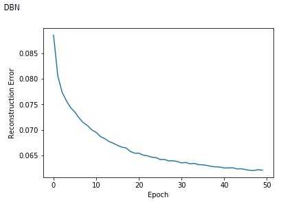
Figure 11-10. Reconstruction errors of the DBN
Figure 11-11 displays the learned features from the last layer of the DBN — the hidden layer of the fourth RBM.
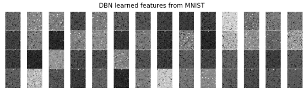
Figure 11-11. Learned features of the fourth RBM in the DBN
Both the reconstruction errors and the learned features look reasonable and similar to the ones from the individual RBMs we analyzed earlier.
How Unsupervised Learning Helps Supervised Learning
So far, all the work we have done training the RBMs and the DBN involve unsupervised learning. We have not used any labels for the images at all.
Instead, we have built generative models by learning relevant latent features from the original MNIST images provided in the 50,000 example training set. These generative models generate images that look reasonably similar to the original images (minimizing the reconstruction error).
Let’s take a step back to understand the usefulness of such a generative model.
Recall that most of the data in the world is unlabeled. Therefore, as powerful and effective as supervised learning is, we need unsupervised learning to help make sense of all the unlabeled data that exists. Supervised learning is not enough.
To demonstrate the usefulness of unsupervised learning, imagine if instead of 50,000 labeled MNIST images in the training set, we had just a fraction - let’s say we had only 5,000 labeled MNIST images.
A supervised learning-based image classifer that had only 5,000 labeled images would not be nearly as effective as a supervised learning-based image classifier that had 50,000 images. The more labeled data we have, the better the machine learning solution.
How does unsupervised learning help in such a situation?
One way unsupervised learning could help is by generating new labeled examples to help supplement the originally labeled dataset.
Then, the supervised learning could occur on a much larger labeled dataset, resulting in a better overall solution.
Generate Images to Build a Better Image Classifier
To simulate this benefit that unsupervised learning is able to provide, let’s reduce our MNIST training dataset to just five thousand labeled examples. We will store the first five thousand images in a dataframe called inputXReduced.
Then, from these five thousand labeled images, we will generate new images from the generative model we just built using a DBN. And, we will do this 20 times over. In other words, we will generate five thousand new images 20 times to create a dataset that is 100,000 large, all of which will be labeled. Technically, we are storing the final hidden layer outputs not the reconstructed images directly, although we will store the reconstructed images, too, so we can evaluate them soon.
We will store these 100,000 outputs in a NumPy array called generatedImages.
# Generate images and store theminputXReduced=X_train.loc[:4999]foriinrange(0,20):("Run ",i)finalOutput_DBN,reconstructedOutput_DBN=dbn.dbn_output(inputXReduced)ifi==0:generatedImages=finalOutput_DBNelse:generatedImages=np.append(generatedImages,finalOutput_DBN,axis=0)
We will loop through the first five thousand labels from the training labels, called y_train, 20 times to generate an array of labels called labels.
# Generate a vector of labels for the generated imagesforiinrange(0,20):ifi==0:labels=y_train.loc[:4999]else:labels=np.append(labels,y_train.loc[:4999])
Finally, we will generate the output on the validation set, which we will need to evaluate the image classifier we build soon.
# Generate images based on the validation setinputValidation=np.array(X_validation)finalOutput_DBN_validation,reconstructedOutput_DBN_validation=\dbn.dbn_output(inputValidation)
Before we use the data we just generated, let’s view a few of the reconstructed images.
# View reconstructed imagesforiinrange(0,10):example=ireconstructedX=pd.DataFrame(data=reconstructedOutput_DBN,\index=X_train[0:5000].index)view_digit(reconstructedX,y_train,example)view_digit(X_train,y_train,example)
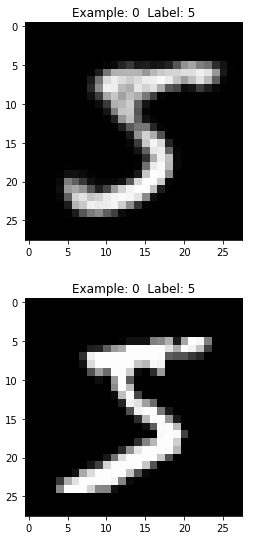
Figure 11-12. First generated image of the DBN
As you can see in Figure 11-12, the generated image is very similar to the original image — both display the digit five. Unlike the RBM generated images we saw earlier, these are more similar to the original MNIST images, including the pixelated bits.
Let’s view a few more images like this to compared the DBN generated ones with the original MNIST ones (see Figures 11-13 through 11-16).
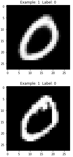
Figure 11-13. Second generated image of the DBN
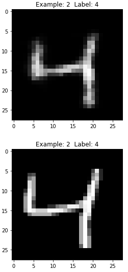
Figure 11-14. Third generated image of the DBN
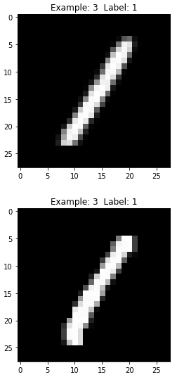
Figure 11-15. Fourth generated image of the DBN
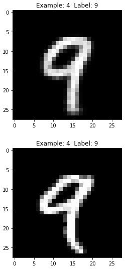
Figure 11-16. Fifth generated image of the DBN
Also, note that the DBN model (as well as the RBM models) is generative and, therefore, the images are produced using a stochastic process. The images are not produced using a deterministic process, and, therefore, the images of a single example vary from one DBN run to another.
To simulate this, we will take the first MNIST image and use the DBN to generate a new one and do this 10 times over.
# Generate the first example 10 timesinputXReduced=X_train.loc[:0]foriinrange(0,10):example=0("Run ",i)finalOutput_DBN_fives,reconstructedOutput_DBN_fives=\dbn.dbn_output(inputXReduced)reconstructedX_fives=pd.DataFrame(data=reconstructedOutput_DBN_fives,\index=[0])("Generated")view_digit(reconstructedX_fives,y_train.loc[:0],example)
As you see from Figures 11-17 through 11-21, all the generated images display the number five, but they vary from image to image even though they all were generated using the same original MNIST image.
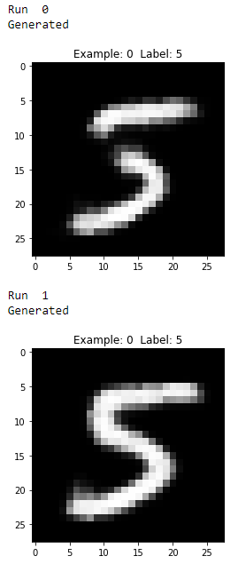
Figure 11-17. First two generated images of the digit five
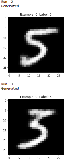
Figure 11-18. Second two generated images of the digit five
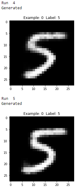
Figure 11-19. Third two generated images of the digit five
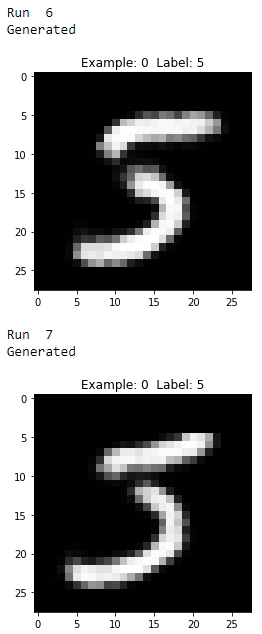
Figure 11-20. Fourth two generated images of the digit five
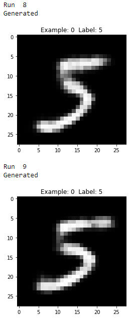
Figure 11-21. Fifth two generated images of the digit five
Image Classifier Using LightGBM
Now, let’s build an image classifier using a supervised learning algorithm we introduced earlier in the book - the gradient boosting algorithm LightGBM.
Supervised Only
The first image classifier will rely on just the first five thousand labeled MNIST images. This is the reduced set from the original 50,000 labeled MNIST training set; we designed this to simulate real world problems where we have relatively few labeled examples.
Since we covered gradient boosting and the LightGBM algorithm in depth earlier in the book, we will not go into a lot of details.
Let’s set the parameters for the algorithm.
predictionColumns=['0','1','2','3','4','5','6','7','8','9']params_lightGB={'task':'train','application':'binary','num_class':10,'boosting':'gbdt','objective':'multiclass','metric':'multi_logloss','metric_freq':50,'is_training_metric':False,'max_depth':4,'num_leaves':31,'learning_rate':0.1,'feature_fraction':1.0,'bagging_fraction':1.0,'bagging_freq':0,'bagging_seed':2018,'verbose':0,'num_threads':16}
Next, we will train on the 5,000 labeled MNIST training set - the reduced set - and validate on the 10,000 labeled MNIST validation set.
trainingScore=[]validationScore=[]predictionsLightGBM=pd.DataFrame(data=[],\index=y_validation.index,\columns=predictionColumns)lgb_train=lgb.Dataset(X_train.loc[:4999],y_train.loc[:4999])lgb_eval=lgb.Dataset(X_validation,y_validation,reference=lgb_train)gbm=lgb.train(params_lightGB,lgb_train,num_boost_round=2000,valid_sets=lgb_eval,early_stopping_rounds=200)loglossTraining=log_loss(y_train.loc[:4999],\gbm.predict(X_train.loc[:4999],num_iteration=gbm.best_iteration))trainingScore.append(loglossTraining)predictionsLightGBM.loc[X_validation.index,predictionColumns]=\gbm.predict(X_validation,num_iteration=gbm.best_iteration)loglossValidation=log_loss(y_validation,predictionsLightGBM.loc[X_validation.index,predictionColumns])validationScore.append(loglossValidation)('Training Log Loss: ',loglossTraining)('Validation Log Loss: ',loglossValidation)loglossLightGBM=log_loss(y_validation,predictionsLightGBM)('LightGBM Gradient Boosting Log Loss: ',loglossLightGBM)
Figure 11-22 shows the training and the validation log loss from this supervised-only solution.
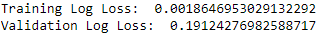
Figure 11-22. Supervised only log loss
Figure 11-23 shows the overall accuracy of this supervised-only image classification solution.
predictionsLightGBM_firm=np.argmax(np.array(predictionsLightGBM),axis=1)accuracyValidation_lightGBM=accuracy_score(np.array(y_validation),\predictionsLightGBM_firm)("Supervised-Only Accuracy: ",accuracyValidation_lightGBM)

Figure 11-23. Supervised only accuracy
Unsupervised and Supervised Solution
Now, instead of training on the 5,000 labeled MNIST images, let’s train on the 100,000 generated images from the DBN.
# Prepare DBN-based DataFrames for LightGBM usegeneratedImagesDF=pd.DataFrame(data=generatedImages,index=range(0,100000))labelsDF=pd.DataFrame(data=labels,index=range(0,100000))X_train_lgb=pd.DataFrame(data=generatedImagesDF,index=generatedImagesDF.index)X_validation_lgb=pd.DataFrame(data=finalOutput_DBN_validation,index=X_validation.index)
# Train LightGBMtrainingScore=[]validationScore=[]predictionsDBN=pd.DataFrame(data=[],index=y_validation.index,columns=predictionColumns)lgb_train=lgb.Dataset(X_train_lgb,labels)lgb_eval=lgb.Dataset(X_validation_lgb,y_validation,reference=lgb_train)gbm=lgb.train(params_lightGB,lgb_train,num_boost_round=2000,valid_sets=lgb_eval,early_stopping_rounds=200)loglossTraining=log_loss(labelsDF,gbm.predict(X_train_lgb,\num_iteration=gbm.best_iteration))trainingScore.append(loglossTraining)predictionsDBN.loc[X_validation.index,predictionColumns]=\gbm.predict(X_validation_lgb,num_iteration=gbm.best_iteration)loglossValidation=log_loss(y_validation,predictionsDBN.loc[X_validation.index,predictionColumns])validationScore.append(loglossValidation)('Training Log Loss: ',loglossTraining)('Validation Log Loss: ',loglossValidation)loglossDBN=log_loss(y_validation,predictionsDBN)('LightGBM Gradient Boosting Log Loss: ',loglossDBN)
Figure 11-24 displays the log loss of this unsupervised-enchanced image classification solution.
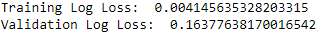
Figure 11-24. Unsupervised plus supervised log loss
Figure 11-25 shows the overall accuracy of this unsupervised-enchanced image classification solution.

Figure 11-25. Unsupervised plus supervised accuracy
As you see, the solution improves by nearly one percentage point, which is considerable.
Conclusion
In Chapter 10, we introduced the first class of generative models called restricted Boltzmann machines (RBMs).
In this chapter, we built upon this concept by introducing more advanced generative models known as deep belief networks (DBNs), which are comprised of multiple RBMs stacked on top of each other.
We demonstrated how DBNs work - in a purely unsupervised manner, the DBN learns the underlying structure of data and uses this learning to generate new synthetic data. Based on how the new synthetic data compares to the original data, the DBN improves its generative ability so much so that the synthetic data increasingly resembles the original data.
We also showed how synthetic data generated by DBNs could supplement existing labeled datasets, improving the performance of supervised learning models by increasing the size of the overall training set.
The semi-supervised solution we developed using DBNs (unsupervised learning) and gradient boosting (supervised learning) outperformed the purely supervised solution in the MNIST image classifaction problem we had.
In Chapter 12, we will introduce one of the latest advances in unsupervised learning (and generative modeling, more specifically) known as generative adversarial networks (GANs).