Data Preparation

Let’s first load the necessary libraries.

# Import libraries
'''Main'''
import numpy as np
import pandas as pd
import os, time
import pickle, gzip

'''Data Viz'''
import matplotlib.pyplot as plt
import seaborn as sns
color = sns.color_palette()
import matplotlib as mpl

%matplotlib inline

'''Data Prep and Model Evaluation'''
from sklearn import preprocessing as pp
from sklearn.model_selection import train_test_split
from sklearn.metrics import precision_recall_curve, average_precision_score
from sklearn.metrics import roc_curve, auc, roc_auc_score

Next, let’s load the dataset and create Pandas dataframes.

# Load the datasets
current_path = os.getcwd()
file = '\\datasets\\mnist_data\\mnist.pkl.gz'

f = gzip.open(current_path+file, 'rb')
train_set, validation_set, test_set = pickle.load(f, encoding='latin1')
f.close()

X_train, y_train = train_set[0], train_set[1]
X_validation, y_validation = validation_set[0], validation_set[1]
X_test, y_test = test_set[0], test_set[1]

# Create Pandas DataFrames from the datasets
train_index = range(0,len(X_train))
validation_index = range(len(X_train), \
                         len(X_train)+len(X_validation))
test_index = range(len(X_train)+len(X_validation), \
                   len(X_train)+len(X_validation)+len(X_test))

X_train = pd.DataFrame(data=X_train,index=train_index)
y_train = pd.Series(data=y_train,index=train_index)

X_validation = pd.DataFrame(data=X_validation,index=validation_index)
y_validation = pd.Series(data=y_validation,index=validation_index)

X_test = pd.DataFrame(data=X_test,index=test_index)
y_test = pd.Series(data=y_test,index=test_index)

K-Means Inertia

Let’s introduce the algorithm. We need to set the number of clusters we would like (n_clusters), the number of initializations we would like to perform (n_init), the maximum number of iterations the algorithm will run to reassign observations to minimize inertia (max_iter), and the tolerance to declare convergence (tol).

We will keep the default values for number of initializations (10), maximum number of iterations (300), and tolerance (0.0001). Also, for now, we will use the first 100 principal components from PCA (cutoff).

To test how the number of clusters we designate affects the inertia measure, let’s run K-means for cluster sizes of 2 through 20 and record the inertia for each.

Here is the code.

# K-means - Inertia as the number of clusters varies
from sklearn.cluster import KMeans

n_clusters = 10
n_init = 10
max_iter = 300
tol = 0.0001
random_state = 2018
n_jobs = 2

kMeans_inertia = pd.DataFrame(data=[],index=range(2,21), \
                              columns=['inertia'])
for n_clusters in range(2,21):
    kmeans = KMeans(n_clusters=n_clusters, n_init=n_init, \
                max_iter=max_iter, tol=tol, random_state=random_state, \
                n_jobs=n_jobs)

    cutoff = 99
    kmeans.fit(X_train_PCA.loc[:,0:cutoff])
    kMeans_inertia.loc[n_clusters] = kmeans.inertia_

As Figure 5-1 shows, the inertia decreases as the number of clusters increases. This makes sense. The more clusters we have, the greater the homogeneity among observations within each cluster. However, fewer clusters are easier to work with than more, so finding the right number of clusters to generate is an important consideration when running K-means.

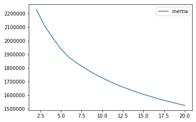
Figure 5-1. K-means inertia for cluster sizes 2 through 20

Evaluating the Clustering Results

To demonstrate how K-means works and how increasing the number of clusters results in more homogenous clusters, let’s define a function to analyze the results of each experiment we do.

The cluster assignments - generated by the clustering algorithm - will be stored in a Pandas DataFrame called clusterDF.

Let’s count the number of observations in each cluster and store these in a Pandas DataFrame called countByCluster.

def analyzeCluster(clusterDF, labelsDF):
    countByCluster = \
        pd.DataFrame(data=clusterDF['cluster'].value_counts())
    countByCluster.reset_index(inplace=True,drop=False)
    countByCluster.columns = ['cluster','clusterCount']

Next, let’s join the clusterDF with the true labels array, which we will call labelsDF.

    preds = pd.concat([labelsDF,clusterDF], axis=1)
    preds.columns = ['trueLabel','cluster']

Let’s also count the number of observations for each true label in the training set - this won’t change but is good for us to know.

    countByLabel = pd.DataFrame(data=preds.groupby('trueLabel').count())

Now, for each cluster, we will count the number of observations for each distinct label within a cluster. For example, if a given cluster has three thousand observations, two thousand may represent the number two, five hundred may represent the number one, three hundred may represent the number zero, and the remaining two hundred may represent the number nine.

Once we calculate these, we will store the count for the most frequently occurring number for each cluster. In the example above, we would store a count of two thousand for this cluster.

    countMostFreq = \
        pd.DataFrame(data=preds.groupby('cluster').agg( \
                        lambda x:x.value_counts().iloc[0]))
    countMostFreq.reset_index(inplace=True,drop=False)
    countMostFreq.columns = ['cluster','countMostFrequent']

Finally, we will judge the success of each clustering run based on how tightly grouped the observations are within each cluster. For example, in the example above, the cluster has two thousand observations that have the same label out of a total of three thousand observations in the cluster.

This cluster is not great since we ideally want to group similar observations together in the same cluster and exclude dissimilar ones from the same cluster.

Let’s define the overall accuracy of the clustering as the sum of the counts of the most frequently occuring observations across all the clusters divided by the total number of observations in the training set (i.e., 50,000).

    accuracyDF = countMostFreq.merge(countByCluster, \
                        left_on="cluster",right_on="cluster")
    overallAccuracy = accuracyDF.countMostFrequent.sum()/ \
                        accuracyDF.clusterCount.sum()

We can also assess the accuracy by cluster.

    accuracyByLabel = accuracyDF.countMostFrequent/ \
                        accuracyDF.clusterCount

For the sake of conciseness, we will have all this code in a single function, available on GitHub.

K-Means Accuracy

Let’s now perform the experiments we did earlier, but, instead of calculating inertia, we will calculate the overall homogeneity of the clusters based on the accuracy measure we’ve defined for this MNIST digits dataset.

# K-means - Accuracy as the number of clusters varies

n_clusters = 5
n_init = 10
max_iter = 300
tol = 0.0001
random_state = 2018
n_jobs = 2

kMeans_inertia = \
    pd.DataFrame(data=[],index=range(2,21),columns=['inertia'])
overallAccuracy_kMeansDF = \
    pd.DataFrame(data=[],index=range(2,21),columns=['overallAccuracy'])

for n_clusters in range(2,21):
    kmeans = KMeans(n_clusters=n_clusters, n_init=n_init, \
                max_iter=max_iter, tol=tol, random_state=random_state, \
                n_jobs=n_jobs)

    cutoff = 99
    kmeans.fit(X_train_PCA.loc[:,0:cutoff])
    kMeans_inertia.loc[n_clusters] = kmeans.inertia_
    X_train_kmeansClustered = kmeans.predict(X_train_PCA.loc[:,0:cutoff])
    X_train_kmeansClustered = \
        pd.DataFrame(data=X_train_kmeansClustered, index=X_train.index, \
                     columns=['cluster'])

    countByCluster_kMeans, countByLabel_kMeans, countMostFreq_kMeans, \
        accuracyDF_kMeans, overallAccuracy_kMeans, accuracyByLabel_kMeans \
        = analyzeCluster(X_train_kmeansClustered, y_train)

    overallAccuracy_kMeansDF.loc[n_clusters] = overallAccuracy_kMeans

Figure 5-2 shows the plot of the overall accuracy for different cluster sizes.

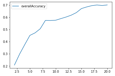
Figure 5-2. K-means accuracy for cluster sizes 2 through 20

As Figure 5-2 shows, the accuracy improves as the number of clusters increases. In other words, clusters become more homogenous as we increase the number of clusters because each cluster becomes smaller and more tightly formed.

Accuracy by cluster varies quite a bit, with some clusters exhibiting a high degree of homogeneity while others less so (see Figure 5-3). For example, in some clusters, over 90% of the images are of the same digit; in other clusters, less than 50% of the images are of the same digit.

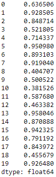
Figure 5-3. K-means accuracy by cluster for cluster size 20

K-Means and the Number of Principal Components

Let’s perform yet another experiment - this time, let’s assess how varying the number of principal components we use in the clustering algorithm impacts the homogeneity of the clusters (defined as accuracy).

In the experiments earlier, we used one hundred principal components, dervied from normal PCA. Recall that the original number of dimensions for the MNIST digits dataset is 784.

If PCA does a good job of capturing the underlying structure in the data as compactly as possible, the clustering algorithm will have an easy time grouping similar images together, regardless of whether the clustering happens on just a fraction of the principal components or many more.

In other words, clustering should perform just as well using 10 or 50 principal components as it does using 100 or several hundred principal components.

Let’s test this hypothesis. We will pass along 10, 50, 100, 200, 300, 400, 500, 600, 700, and 784 principal components and gauge the accuracy of each clustering experiment. We will then plot these results to see how varying the number of principal components affects clustering accuracy.

# K-means - Accuracy as the number of components varies

n_clusters = 20
n_init = 10
max_iter = 300
tol = 0.0001
random_state = 2018
n_jobs = 2

kMeans_inertia = pd.DataFrame(data=[],index=[9, 49, 99, 199, \
                    299, 399, 499, 599, 699, 784],columns=['inertia'])

overallAccuracy_kMeansDF = pd.DataFrame(data=[],index=[9, 49, \
                    99, 199, 299, 399, 499, 599, 699, 784], \
                    columns=['overallAccuracy'])

for cutoffNumber in [9, 49, 99, 199, 299, 399, 499, 599, 699, 784]:
    kmeans = KMeans(n_clusters=n_clusters, n_init=n_init, \
                max_iter=max_iter, tol=tol, random_state=random_state, \
                n_jobs=n_jobs)

    cutoff = cutoffNumber
    kmeans.fit(X_train_PCA.loc[:,0:cutoff])
    kMeans_inertia.loc[cutoff] = kmeans.inertia_
    X_train_kmeansClustered = kmeans.predict(X_train_PCA.loc[:,0:cutoff])
    X_train_kmeansClustered = pd.DataFrame(data=X_train_kmeansClustered, \
                                index=X_train.index, columns=['cluster'])

    countByCluster_kMeans, countByLabel_kMeans, countMostFreq_kMeans, \
        accuracyDF_kMeans, overallAccuracy_kMeans, accuracyByLabel_kMeans \
        = analyzeCluster(X_train_kmeansClustered, y_train)

    overallAccuracy_kMeansDF.loc[cutoff] = overallAccuracy_kMeans

Figure 5-4 shows the plot of the clustering accuracy at the different number of principal components.

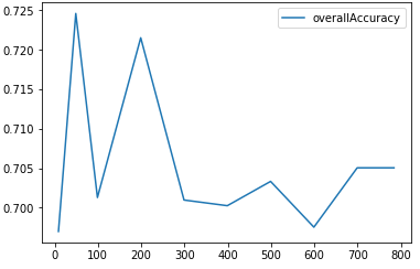
Figure 5-4. K-means clustering accuracy as number of principal components varies

This plot supports our hypothesis. As the number of principal components varies from 10 to 784, the clustering accuracy remains stable and consistent around 70%.

This is one reason why clustering should be performed on dimensionality reduced datasets - the clustering algorithms generally perform better, both in terms of time and clustering accuracy, on dimensionality reduced datasets.

In our case, for the MNIST dataset, the original 784 dimensions are not too unmanageable for a clustering algorithm, but imagine if the original dataset were thousands or millions of dimensions large. The case for reducing the dimensionality before performing clustering is even stronger in such a scenario.

K-Means on the Original Dataset

To make this point clearer, let’s perform clustering on the original dataset and measure how varying the number of dimensions we pass into the clustering algorithm affects clustering accuracy.

For the PCA-reduced dataset in the previous section, varying the number of principal components that we pass into the clustering algorithm did not affect clustering accuracy, which remained stable and consistent at approximately 70%.

Is this true for the original dataset, too?

# K-means - Accuracy as the number of components varies
# On the original MNIST data (not PCA-reduced)

n_clusters = 20
n_init = 10
max_iter = 300
tol = 0.0001
random_state = 2018
n_jobs = 2

kMeans_inertia = pd.DataFrame(data=[],index=[9, 49, 99, 199, \
                    299, 399, 499, 599, 699, 784],columns=['inertia'])

overallAccuracy_kMeansDF = pd.DataFrame(data=[],index=[9, 49, \
                    99, 199, 299, 399, 499, 599, 699, 784], \
                    columns=['overallAccuracy'])

for cutoffNumber in [9, 49, 99, 199, 299, 399, 499, 599, 699, 784]:
    kmeans = KMeans(n_clusters=n_clusters, n_init=n_init, \
                max_iter=max_iter, tol=tol, random_state=random_state, \
                n_jobs=n_jobs)

    cutoff = cutoffNumber
    kmeans.fit(X_train.loc[:,0:cutoff])
    kMeans_inertia.loc[cutoff] = kmeans.inertia_
    X_train_kmeansClustered = kmeans.predict(X_train.loc[:,0:cutoff])
    X_train_kmeansClustered = pd.DataFrame(data=X_train_kmeansClustered, \
                                index=X_train.index, columns=['cluster'])

    countByCluster_kMeans, countByLabel_kMeans, countMostFreq_kMeans, \
        accuracyDF_kMeans, overallAccuracy_kMeans, accuracyByLabel_kMeans \
        = analyzeCluster(X_train_kmeansClustered, y_train)

    overallAccuracy_kMeansDF.loc[cutoff] = overallAccuracy_kMeans

Figure 5-5 shows the plot of the clustering accuracy at the different number of original dimensions.

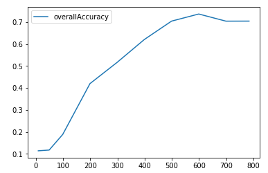
Figure 5-5. K-means clustering accuracy as nNumber of original dimensions varies

As the plot shows, clustering accuracy is very poor at few dimensions and improves to nearly 70% only as the number of dimensions climb to six hundred dimensions.

In the PCA case, clustering accuracy was approximately 70% even at 10 dimensions, demonstrating the power of dimensionality reduction to densely capture salient information in the original dataset.

Agglomerative Hierarchical Clustering

The version of hierarchical clustering we will explore is called agglomerative clustering. Although Scikit-Learn has a library for this, it performs very slowly.

Instead, we will choose to use another version of this called fastcluster. This package is a C++ library with an interface in Python/SciPy.³

The main function that we will use in this package is fastcluster.linkage_vector. This requires several arguments, including the training matrix X, the method, and the metric.

The method - which can be set to single, centroid, median, or ward - specifies which clustering scheme to use to determine the distance from a new node in the dendrogram to the other nodes.

And, the metric should be set to euclidean in most cases, and it is required to be euclidean if the method is centroid, median, or ward. For more on these arguments, please refer to the fastcluster documentation.

Let’s set up the hierarchical clustering algorithm for our data. As before, we will train the algorithm on the first one hundred principal components from the PCA-reduced MNIST image dataset. We will set the method to ward (which performed the best, by far, in the experimentation), and the metric to euclidean.

Ward stands for Ward’s minimum variance method and more information on the method is available online. Ward is a good default choice to use in hierarchical clustering, but, as always, it is best to experiment for your specific datasets in practice.

import fastcluster
from scipy.cluster.hierarchy import dendrogram, cophenet
from scipy.spatial.distance import pdist

cutoff = 100
Z = fastcluster.linkage_vector(X_train_PCA.loc[:,0:cutoff], \
                               method='ward', metric='euclidean')
Z_dataFrame = pd.DataFrame(data=Z, \
    columns=['clusterOne','clusterTwo','distance','newClusterSize'])

The hierarchical clustering algorithm will return a matrix Z.

The algorithm treats each observation in our 50,000 MNIST digits dataset as a single-point cluster, and, in each iteration of training, the algorithm will merge the two clusters that have the smallest distance between them.

Initially, the algorithm is just merging single point clusters together, but, as it proceeds, it will merge multi-point clusters with either single point or multi-point clusters.

Eventually, through this iterative process, all the clusters are merged together, forming the trunk in the upside-down tree (dendrogram).

The Dendrogram

Figure 5-6 shows the matrix Z that was generated by the clustering algorithm; please refer to it for more intution on what the algorithm accomplishes.

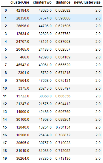
Figure 5-6. First few rows of Z matrix of hierarchical clustering

The first two columns, clusterOne and clusterTwo, in this table lists which two clusters (could be single point clusters - the original observations - or multi point clusters) are being merged given their distance relative to each other.

The third column, distance, displays this distance, which was determined by the Ward method and euclidean metric that we passed into the clustering algorithm.

As you can see, the distance is monotonically increasing. In other words, the shortest-distance clusters are merged first, and the algorithm iteratively merges the next shortest-distance clusters until all the points have been joined into a single cluster at the top of the dendrogram.

Initially, the algorithm merges single point clusters together, forming new clusters with a size of two, as shown in the fourth column, newClusterSize.

However, as we get much further along, the algorithm joins large multi point clusters with other large multi point clusters, as shown in Figure 5-7. At the very last iteration - 49,998 - two large clusters are joined together, forming a single cluster - the top tree trunk - with all 50,000 original observations.

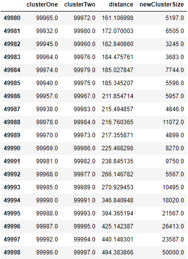
Figure 5-7. Last few rows of Z matrix of hierarchical clustering

You may be a bit confused by the clusterOne and clusterTwo entries in this table. For example, in the last row - 49,998 - cluster 99,996 is joined with cluster 99,997. But, as you know, there are only 50,000 observations in the MNIST digits dataset.

clusterOne and clusterTwo refer to the original observations for numbers 0 through 49,999. For numbers above 49,999, the cluster numbers refer to previously clustered points. For example, 50,000 refers to the newly formed cluster in row 0, 50,001 refers to the newly formed cluster in row 1, etc.

In row 49,998, clusterOne, 99,996, refers to the cluster formed in row 49,996, and clusterTwo, 99,997, refers to the cluster formed in row 49,997. You can continue to work your way through this table using this formula to see how the clusters are being joined.

Evaluating the Clustering Results

Now that we have the dendrogram in place, let’s determine where to cut off the dendrogram to have the number of clusters we desire. To more easily compare hierarchical clustering results with those of K-means, let’s cut the dendrogram to have exactly 20 clusters.

We will then use the clustering accuracy metric - defined in the K-means section - to judge how homogenous the hierarchical clustering clusters are.

To create the clusters we desire from the dendrogram, let’s pull in the fcluster library from SciPy. We need to specify the distance threshold to cut off the dendrogram; this will determine how many distinct clusters we are left with.

Remember that the larger the distance threshold, the fewer clusters we will have. A large distance threshold is akin to cutting the upside-down tree at a very high vertical point. Since more and more of the points are grouped together the higher up the tree we go, the fewer clusters we will have.

To get exactly 20 clusters, we need to experiment with the distance threshold, which I have done for us already.

The fcluster library will take our dendrogram and cut it with the distance threshold we specify. Each observation in the 50,000 observations MNIST digits dataset will get a cluster label, and we will store these in a Pandas DataFrame.

from scipy.cluster.hierarchy import fcluster

distance_threshold = 160
clusters = fcluster(Z, distance_threshold, criterion='distance')
X_train_hierClustered = \
    pd.DataFrame(data=clusters,index=X_train_PCA.index,columns=['cluster'])

Let’s verify that there are exactly 20 distinct clusters, given our choice of the distance threshold.

print("Number of distinct clusters: ", \
      len(X_train_hierClustered['cluster'].unique()))

Figure 5-8 confirms the 20 clusters, as expected.

Figure 5-8. Number of distinct clusters for hierarchical clustering

Now, let’s evaluate the results.

countByCluster_hierClust, countByLabel_hierClust, \
    countMostFreq_hierClust, accuracyDF_hierClust, \
    overallAccuracy_hierClust, accuracyByLabel_hierClust \
    = analyzeCluster(X_train_hierClustered, y_train)

print("Overall accuracy from hierarchical clustering: ", \
      overallAccuracy_hierClust)

As shown in Figure 5-9, the overall accuracy is approximately 77%, even better than the approximately 70% accuracy from K-means.

Figure 5-9. Overall accuracy for hierarchical clustering

Let’s also assess the accuracy by cluster.

As shown in Figure 5-10, the accuracy varies quite a bit. For some clusters, the accuracy is remarkably high, nearly 100%. For some, the accuracy is shy of 50%.

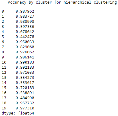
Figure 5-10. Accuracy by cluster for hierarchical clustering

Overall, hierarchical clustering performs well on the MNIST digits dataset.

Remember that we accomplished this without using any labels.

This is how it would work on real world examples: we would apply dimensionality reduction first (such as PCA), then we would perform clustering (such as hierarchical clustering), and finally we would hand-label a few points per cluster.

For example, for this MNIST digits dataset, if we did not have any labels, we would look at a few images per cluster and label those images based on the digit they displayed. So long as the clusters were homogenous enough, the few hand labels we would generate could be applied automatically to all the other images in the cluster.

All of a sudden, without too much effort, we would have labeled all the images in our 50,000 dataset with a near 77% accuracy. This is impressive and highlights the power of unsupervised learning.

DBSCAN Algorithm

Let’s first use the DBSCAN library from Scikit-Learn. We need to specify the maximum distance (called eps) between two points for them to be considered as in the same neighborhood and the minimum samples (called min_samples) for a group to be called a cluster.

The default value for eps is 0.5, and the default value for min_samples is 5.

If eps is set too low, no points may be close enough to other points for them to be considered in the same neighborhood. Hence, all the points would remain unclustered.

If eps is set too high, many points may be clustered and only a handful of points would remain unclustered, effectively being labeled as the outliers in the dataset.

We need to search for the optimal eps for our MNIST digits dataset.

min_samples designates how many points need to be within the eps distance in order for the points to be called a cluster. Once there are min_samples number of closely located points, any other point that is within the eps distance of any of these so-called core points is part of that cluster, even if those other points do not have the min_samples number of points within eps distance around them.

These other points - if they do not have the min_samples number of points within eps distance around them - are called the border points of the cluster.

Generally, as the min_samples increases, the fewer clusters we will have. As with eps, we need to search for the optimal min_samples for our MNIST digits dataset.

As you can see, the clusters have core points and border points, but, for all intents and purposes, they belong to the same group. All points that do not get grouped - either as core or border points of a cluster - are labeled as outliers.

Applying DBSCAN to Our Dataset

Let’s now move to our specific problem. As before, we will apply DBSCAN to the first one hundred principal components of the PCA-reduced MNIST digits dataset.

from sklearn.cluster import DBSCAN

eps = 3
min_samples = 5
leaf_size = 30
n_jobs = 4

db = DBSCAN(eps=eps, min_samples=min_samples, leaf_size=leaf_size,
            n_jobs=n_jobs)

cutoff = 99
X_train_PCA_dbscanClustered = db.fit_predict(X_train_PCA.loc[:,0:cutoff])
X_train_PCA_dbscanClustered = \
    pd.DataFrame(data=X_train_PCA_dbscanClustered, index=X_train.index, \
                 columns=['cluster'])

countByCluster_dbscan, countByLabel_dbscan, countMostFreq_dbscan, \
    accuracyDF_dbscan, overallAccuracy_dbscan, accuracyByLabel_dbscan \
    = analyzeCluster(X_train_PCA_dbscanClustered, y_train)

overallAccuracy_dbscan

We will keep the min_samples at the default value of five, but we will adjust the eps to three to avoid having too few points clustered.

Figure 5-11 shows the overall accuracy.

Figure 5-11. Overall accuracy for DBSCAN

As you can see, the accuracy is very poor compared to K-means and hierarchical clustering. We can fidget with the parameters eps and min_samples to improve the results, but it appears that DBSCAN is poorly suited to cluster the observations for this particular dataset.

To explore why, let’s look at the clusters (see Figure 5-12).

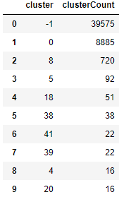
Figure 5-12. Cluster results for DBSCAN

Most of the points are unclustered. You can see this in the plot. 39,651 points - out of the 50,000 observations in the training set - are in cluster -1, which means that they do not belong to any cluster. They are labeled as outliers - noise, in other words.

8,885 points belong in cluster 0. Then, there is a long tail of smaller-sized clusters. It appears that DBSCAN has a hard time finding distinct dense groups of points, and, therefore, it does a poor job of clustering the MNIST images based on the digit they display.

HDBSCAN

Let’s try another version of DBSCAN and see if the results improve. This one is known as HDBSCAN, or hierarchical DBSCAN. The takes the DBSCAN algorithm we introduced and converts it into a hierarchical clustering algorithm.

In other words, it groups based on density and then links the density-based clusters based on distance iteratively, like in the hierarchical clustering algorithm we introduced in an earlier section.

The two main parameters for this algorithm are min_cluster_size and min_samples, which defaults to min_cluster_size when set to None.

Let’s use the out-of-the-box parameter selections and gauge if HDBSCAN performs better than DBSCAN did for our MNIST digits dataset.

import hdbscan

min_cluster_size = 30
min_samples = None
alpha = 1.0
cluster_selection_method = 'eom'

hdb = hdbscan.HDBSCAN(min_cluster_size=min_cluster_size, \
        min_samples=min_samples, alpha=alpha, \
        cluster_selection_method=cluster_selection_method)

cutoff = 10
X_train_PCA_hdbscanClustered = \
    hdb.fit_predict(X_train_PCA.loc[:,0:cutoff])

X_train_PCA_hdbscanClustered = \
    pd.DataFrame(data=X_train_PCA_hdbscanClustered, \
    index=X_train.index, columns=['cluster'])

countByCluster_hdbscan, countByLabel_hdbscan, \
    countMostFreq_hdbscan, accuracyDF_hdbscan, \
    overallAccuracy_hdbscan, accuracyByLabel_hdbscan \
    = analyzeCluster(X_train_PCA_hdbscanClustered, y_train)

Figure 5-13 shows the overall accuracy.

Figure 5-13. Overall accuracy for HDBSCAN

At 25%, this is only marginally better than that of DBSCAN and well short of the 70%-plus achieved by K-means and hierarchical clustering.

Figure 5-14 displays the accuracy of the various clusters.

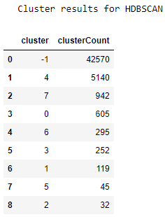
Figure 5-14. Cluster results for HDBSCAN

We see a similar phenomenon as we did in DBSCAN. Most points are unclustered, and then there is a long tail of small-sized clusters. The results do not improve much.