Lending Club Data

For this chapter, we will use loan data from Lending Club, a U.S. peer-to-peer lending company. Borrowers on the platform can borrow between $1,000 to $40,000 in the form of unsecured personal loans, for a term of either three or five years.

Investors can browse the loan applications and choose to finance the loans based on the credit history of the borrower, the amount of the loan, the loan grade, and the purpose of the loan.

Investors earn money through interest paid on the loans, and Lending Club makes money from a loan origination fee and service charges.

The loan data we will use is from 2007-2011 and is made publicly available on the Lending Club website. A data dictionary is also available via the same link.

Data Preparation

Like in previous chapters, let’s prepare the environment to work with the Lending Club data.

Load libraries

First, let’s load the necessary libraries.

# Import libraries
'''Main'''
import numpy as np
import pandas as pd
import os, time, re
import pickle, gzip

'''Data Viz'''
import matplotlib.pyplot as plt
import seaborn as sns
color = sns.color_palette()
import matplotlib as mpl

%matplotlib inline

'''Data Prep and Model Evaluation'''
from sklearn import preprocessing as pp
from sklearn.model_selection import train_test_split
from sklearn.metrics import precision_recall_curve, average_precision_score
from sklearn.metrics import roc_curve, auc, roc_auc_score

'''Algorithms'''
from sklearn.decomposition import PCA
from sklearn.cluster import KMeans
import fastcluster
from scipy.cluster.hierarchy import dendrogram, cophenet, fcluster
from scipy.spatial.distance import pdist

Explore the data

Next, let’s load the loan data and designate which of the columns to keep.

The original loan data file has 144 columns, but the vast majority of these columns are empty and are of little value to us. Therefore, we will designate a subset of the columns that are mostly populated and are worth using in our clustering application.

These fields include attributes of the loan such as the amount requested, the amount funded, the term, the interest rate, the loan grade, etc. and attributes of the borrower such as employment length, home ownership status, annual income, address, and purpose for borrowing money.

We will also explore the data a bit.

# Load the data
current_path = os.getcwd()
file = '\\datasets\\lending_club_data\\LoanStats3a.csv'
data = pd.read_csv(current_path + file)

# Select columns to keep
columnsToKeep = ['loan_amnt','funded_amnt','funded_amnt_inv','term', \
                 'int_rate','installment','grade','sub_grade', \
                 'emp_length','home_ownership','annual_inc', \
                 'verification_status','pymnt_plan','purpose', \
                 'addr_state','dti','delinq_2yrs','earliest_cr_line', \
                 'mths_since_last_delinq','mths_since_last_record', \
                 'open_acc','pub_rec','revol_bal','revol_util', \
                 'total_acc','initial_list_status','out_prncp', \
                 'out_prncp_inv','total_pymnt','total_pymnt_inv', \
                 'total_rec_prncp','total_rec_int','total_rec_late_fee', \
                 'recoveries','collection_recovery_fee','last_pymnt_d', \
                 'last_pymnt_amnt']

data = data.loc[:,columnsToKeep]

data.shape

data.head()

Figure 6-1 shows the shape of the data: 42542 loans and 37 features.

Figure 6-1. Shape of the loan data

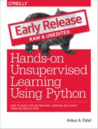
Figure 6-2 previews the data.

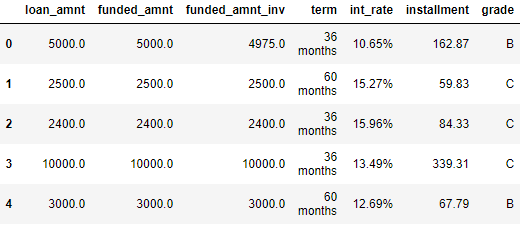
Figure 6-2. First few rows of the loan data

# Transform features from string to numeric
for i in ["term","int_rate","emp_length","revol_util"]:
    data.loc[:,i] = \
        data.loc[:,i].apply(lambda x: re.sub("[^0-9]", "", str(x)))
    data.loc[:,i] = pd.to_numeric(data.loc[:,i])

Impute Missing Values

Let’s find these numerical features and count the number of NaNs per feature. We will then impute these NaNs with either the mean of the feature or, in some cases, just the number zero, depending on what the feature represents from a business perspective.

# Determine which features are numerical
numericalFeats = [x for x in data.columns if data[x].dtype != 'object']

# Display NaNs by feature
nanCounter = np.isnan(data.loc[:,numericalFeats]).sum()
nanCounter

Figure 6-3 shows the number of NaNs by feature.

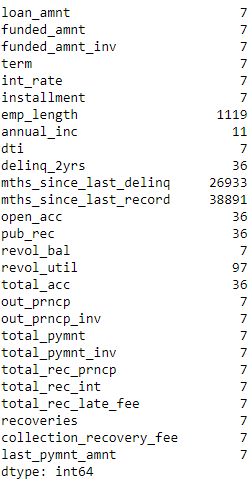
Figure 6-3. Count of NaNs by feature

Most features have a few NaNs, and some - such as the months since last delinquency and last change in record - have many.

Let’s impute these so we do not have to deal with any NaNs during the clustering process.

# Impute NaNs with mean
fillWithMean = ['loan_amnt','funded_amnt','funded_amnt_inv','term', \
                'int_rate','installment','emp_length','annual_inc',\
                'dti','open_acc','revol_bal','revol_util','total_acc',\
                'out_prncp','out_prncp_inv','total_pymnt', \
                'total_pymnt_inv','total_rec_prncp','total_rec_int', \
                'last_pymnt_amnt']

# Impute NaNs with zero
fillWithZero = ['delinq_2yrs','mths_since_last_delinq', \
                'mths_since_last_record','pub_rec','total_rec_late_fee', \
                'recoveries','collection_recovery_fee']

# Perform imputation
im = pp.Imputer(strategy='mean')
data.loc[:,fillWithMean] = im.fit_transform(data[fillWithMean])

data.loc[:,fillWithZero] = data.loc[:,fillWithZero].fillna(value=0,axis=1)

Let’s recalculate the NaNs to make sure no NaNs remain.

As Figure 6-4 shows, we are now safe. All the NaNs have been filled.

numericalFeats = [x for x in data.columns if data[x].dtype != 'object']

nanCounter = np.isnan(data.loc[:,numericalFeats]).sum()
nanCounter

Figure 6-4. Count of NaNs by feature

# Feature engineering
data['installmentOverLoanAmnt'] = data.installment/data.loan_amnt
data['loanAmntOverIncome'] = data.loan_amnt/data.annual_inc
data['revol_balOverIncome'] = data.revol_bal/data.annual_inc
data['totalPymntOverIncome'] = data.total_pymnt/data.annual_inc
data['totalPymntInvOverIncome'] = data.total_pymnt_inv/data.annual_inc
data['totalRecPrncpOverIncome'] = data.total_rec_prncp/data.annual_inc
data['totalRecIncOverIncome'] = data.total_rec_int/data.annual_inc

newFeats = ['installmentOverLoanAmnt','loanAmntOverIncome', \
            'revol_balOverIncome','totalPymntOverIncome', \
           'totalPymntInvOverIncome','totalRecPrncpOverIncome', \
            'totalRecIncOverIncome']

# Select features for training
numericalPlusNewFeats = numericalFeats+newFeats
X_train = data.loc[:,numericalPlusNewFeats]

# Scale data
sX = pp.StandardScaler()
X_train.loc[:,:] = sX.fit_transform(X_train)

Designate Labels for Evaluation

Clustering is an unsupervising learning approach, and, therefore, labels are not used. However, to judge the goodness of our clustering algorithm at finding distinct and homogenous groups of borrowers in this Lending Club dataset, we will use the loan grade as a proxy label.

The loan grade is currently graded by letters, with loan grade “A” as the most credit-worthy and safe and loan grade “G” as the least (see Figure 6-5).

labels = data.grade
labels.unique()

Figure 6-5. Loan grade

There are some NaNs in the loan grade. We will fill these with a value of “Z” and then use the LabelEncoder from Scikit-Learn to transform the letter grades to numerical grades.

To remain consistent, we will load these labels into a “y_train” Python Series.

# Fill missing labels
labels = labels.fillna(value="Z")

# Convert labels to numerical values
lbl = pp.LabelEncoder()
lbl.fit(list(labels.values))
labels = pd.Series(data=lbl.transform(labels.values), name="grade")

# Store as y_train
y_train = labels

labelsOriginalVSNew = pd.concat([labels, data.grade],axis=1)
labelsOriginalVSNew

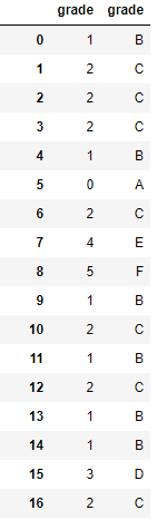
Figure 6-6. Numerical versus letter loan grades

As you can see from Figure 6-6, all the “A” grades have been transformed into 0, the “B” grades into 1, etc.

Let’s also check whether grade “A” loans generally have the least interest rate charged since they are the least risky/most creditworthy while the other loans are charged progressively higher rates of interest.

# Compare loan grades with interest rates
interestAndGrade = pd.DataFrame(data=[data.int_rate,labels])
interestAndGrade = interestAndGrade.T

interestAndGrade.groupby("grade").mean()

Figure 6-7 confirms this. Higher letter grade loans have higher interest rates.¹

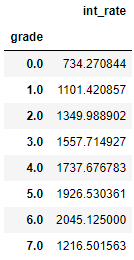
Figure 6-7. Grade versus interest rate

Goodness of the Clusters

Now the data is ready. We have a X_train with all of our 34 numerical features and a y_train with the numerical loan grades, which we use only to validate the results, not to train with the algorithm as you would do in a supervised machine learning problem.

Before we build our first clustering application, let’s introduce a function to analyze the goodness of the clusters we generate using the clustering algorithms.

Specifically, we will use the concept of homogeneity to assess how good each cluster is.

If the clustering algorithm does a good job separating the borrowers in the Lending Club dataset, each cluster should have borrowers that are very similar to each other and not so similar to those in other groups.

Presumably, borrowers that are similar to each other and, therefore, grouped together should have similar credit profiles - in other words, their creditworthiness should be similar.

If this is the case - and with real world problems, a lot of these assumptions are only partially true - borrowers in a given cluster should generally be assigned the same numerical loan grade, which we will validate using the numerical loan grades we set aside in y_train.

The higher the percentage of borrowers that have the most frequently occurring numerical loan grade in each and every cluster, the better the clustering application.

As an example, consider a cluster with one hundred borrowers. If 30 borrowers have a numerical loan grade of 0, 25 borrowers have a loan grade of 1, 20 borrowers have a loan grade of 2, and the remaining borrowers have loan grades ranging from 3 to 7, we would say that the cluster has a 30% accuracy, given that the most frequently occuring loan grade for that cluster applies to just 30% of the borrowers in that cluster.

If we did not have a y_train with the numerical loan grades to validate the goodness of the clusters, we could use an alternative approach. We could sample a few borrowers in each cluster, determine the numerical loan grade for them by hand, and determine if we would give the roughly the same numerical loan grade to those borrowers.

If yes, then the cluster is a good cluster - it is homogenous enough that we would give roughly the same numerical loan grade to the borrowers we sampled.

If not, then the cluster is not good enough - the borrowers are a bit too heterogenous, and we should try to improve the solution using more data, a different clustering algorithm, etc.

We won’t have to sample and manually hand label the borrowers, though, given that we have the numerical loan grades already, but this is important to keep in mind in case you do not have labels at all for your particular problem.

Here is the function to analyze the clusters.

def analyzeCluster(clusterDF, labelsDF):
    countByCluster = \
        pd.DataFrame(data=clusterDF['cluster'].value_counts())
    countByCluster.reset_index(inplace=True,drop=False)
    countByCluster.columns = ['cluster','clusterCount']

    preds = pd.concat([labelsDF,clusterDF], axis=1)
    preds.columns = ['trueLabel','cluster']

    countByLabel = pd.DataFrame(data=preds.groupby('trueLabel').count())

    countMostFreq = pd.DataFrame(data=preds.groupby('cluster').agg( \
        lambda x:x.value_counts().iloc[0]))
    countMostFreq.reset_index(inplace=True,drop=False)
    countMostFreq.columns = ['cluster','countMostFrequent']

    accuracyDF = countMostFreq.merge(countByCluster, \
        left_on="cluster",right_on="cluster")

    overallAccuracy = accuracyDF.countMostFrequent.sum()/ \
        accuracyDF.clusterCount.sum()

    accuracyByLabel = accuracyDF.countMostFrequent/ \
        accuracyDF.clusterCount

    return countByCluster, countByLabel, countMostFreq, \
        accuracyDF, overallAccuracy, accuracyByLabel

K-Means Application

Our first clustering application using this Lending Club dataset will use K-means, which we introduced in Chapter 5. Recall that in K-means clustering, we need to specify the desired clusters K, and the algorithm will assign each borrower to exactly one of these K clusters.

The algorithm will accomplish this my minimizing the within-cluster variation, which is also known as inertia, such that the sum of the within-cluster variations across all K clusters is as small as possible.

Instead of specifying just one value of K, we will run an experiment where we set K from a range of 10 to 30 and plot the results of the accuracy measure we defined in the previous section.

Based on which K measure performs best, we can build the pipeline for clustering using this best-performing K measure.

from sklearn.cluster import KMeans

n_clusters = 10
n_init = 10
max_iter = 300
tol = 0.0001
random_state = 2018
n_jobs = 2

kmeans = KMeans(n_clusters=n_clusters, n_init=n_init, \
                max_iter=max_iter, tol=tol, \
                random_state=random_state, n_jobs=n_jobs)

kMeans_inertia = pd.DataFrame(data=[],index=range(10,31), \
                              columns=['inertia'])

overallAccuracy_kMeansDF = pd.DataFrame(data=[], \
    index=range(10,31),columns=['overallAccuracy'])

for n_clusters in range(10,31):
    kmeans = KMeans(n_clusters=n_clusters, n_init=n_init, \
                    max_iter=max_iter, tol=tol, \
                    random_state=random_state, n_jobs=n_jobs)

    kmeans.fit(X_train)
    kMeans_inertia.loc[n_clusters] = kmeans.inertia_
    X_train_kmeansClustered = kmeans.predict(X_train)
    X_train_kmeansClustered = pd.DataFrame(data= \
        X_train_kmeansClustered, index=X_train.index, \
        columns=['cluster'])

    countByCluster_kMeans, countByLabel_kMeans, \
    countMostFreq_kMeans, accuracyDF_kMeans, \
    overallAccuracy_kMeans, accuracyByLabel_kMeans = \
    analyzeCluster(X_train_kmeansClustered, y_train)

    overallAccuracy_kMeansDF.loc[n_clusters] = \
        overallAccuracy_kMeans

Figure 6-8 displays the plot of the results.

overallAccuracy_kMeansDF.plot()

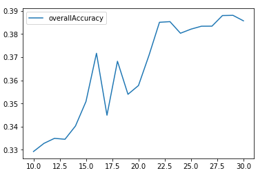
Figure 6-8. Overall accuracy for different Ks using K-means

As we can see, the accuracy is best around 30 clusters and levels out there at approximately 39%.

In other words, for any given cluster, the most-frequently occurring label for that cluster applies to approximately 39% of the borrowers. The remaining 61% of the borrowers have labels that are not the most-frequently occurring label.

Figure 6-9 displays the accuracy by cluster for k=30.

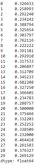
Figure 6-9. Accuracy by cluster using K-means for K=30

The accuracy varies quite a bit cluster by cluster. Some clusters are much more homogenous than others. For example, cluster seven has an accuracy of 76%, while cluster 12 has an accuracy of just 21%.

This is a starting point to build a clustering application to automatically assign new borrowers that apply for a Lending Club loan into a pre-existing group based on how similar they are to other borrowers.

Based on this clustering, it is possible to automatically assign a tentative numerical loan grade to the new borrower, which will be correct approximately 39% of the time.

This is not the best possible solution, and we should consider whether acquiring more data, performing more feature engineering and selection, selecting different parameters for the K-means algorithm, or changing to a different clustering algorithm will improve the results.

It is possible that we do not have enough data to meaningfully separate the borrowers into distinct and homogenous groups materially more than we have already; if this is the case, more data and more feature engineering and selection are required.

Or, it could be that, for the limited data that we have, K-means is not best suited to performing this separation.

Let’s switch to hierarchical clustering to see if our results improve.

Hierarchical Clustering Application

Recall that in hierarchical clustering we do not need to pre-commit to a particular number of clusters. Instead, we can choose how many clusters we would like after the hierarchical clustering has finished running.

Hierarchical clustering will build a dendrogram, which can be conceptually viewed as an upside-down tree. The leaves at the very bottom are the individual borrowers that apply for loans on Lending Club.

Hierarchical clustering joins the borrowers together as we move vertically up the upside-down tree based on how similar they are to each other. The borrowers that are most similar to each other are joined sooner, while borrowers that are not as similar are joined much later. Eventually, all the borroweres are joined together at the very top - the trunk - of the upside down tree.

From a business perspective, this clustering process is clearly very powerful. If we are able to find borrowers that are similar to each other and group them together, we can more efficiently assign creditworthiness ratings to them. We can also have specific strategies for distinct groups of borrowers and better manage them from a relationship perspective, providing better overall client service.

Once the hierarchical clustering algorithm finishes running, we can determine where we want to cut the tree. The lower we cut, the more groups of borrowers we are left with.

Let’s first train the hierarchical clustering algorithm like we did in Chapter 5.

import fastcluster
from scipy.cluster.hierarchy import dendrogram
from scipy.cluster.hierarchy import cophenet
from scipy.spatial.distance import pdist

Z = fastcluster.linkage_vector(X_train, method='ward', \
                               metric='euclidean')

Z_dataFrame = pd.DataFrame(data=Z,columns=['clusterOne', \
                'clusterTwo','distance','newClusterSize'])

<bottom_most_leaves_of_hierarchical_clustering>> shows what the output dataframe looks like. The first few rows are the initial linkages of the bottom-most borrowers.

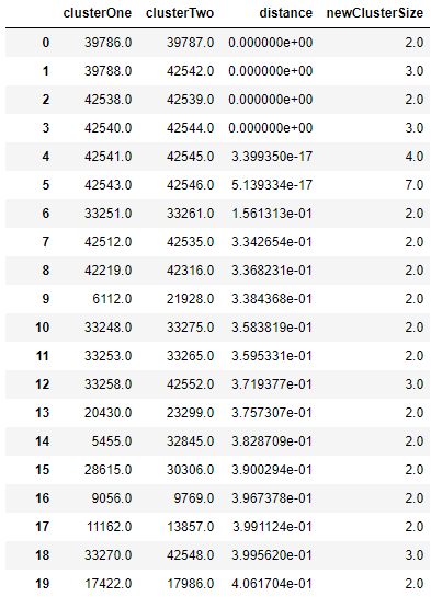
Figure 6-10. Bottom most leaves of hierarchical clustering

Recall that the last few rows represent the top of the upside-down tree, and all 42,541 borrowers are combined together eventually (see Figure 6-11).

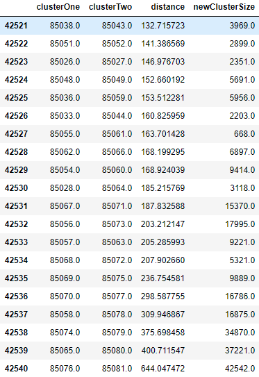
Figure 6-11. Top most leaves of hierarchical clustering

Now, let’s cut the dendrogram so that we are left with a manageable number of clusters. This is set based on the distance_threshold. Based on trial and error, a distance_threshold of 100 results in 32 clusters, which is what we will use for this example.

from scipy.cluster.hierarchy import fcluster
distance_threshold = 100
clusters = fcluster(Z, distance_threshold, criterion='distance')
X_train_hierClustered = pd.DataFrame(data=clusters,
 index=X_train_PCA.index,columns=['cluster'])

print("Number of distinct clusters: ",
 len(X_train_hierClustered['cluster'].unique()))

Figure 6-12 shows the number of distinct clusters given the distance threshold we picked.

Figure 6-12. Number of distinct clusters from hierarchical clustering

countByCluster_hierClust, countByLabel_hierClust, countMostFreq_hierClust,
 accuracyDF_hierClust, overallAccuracy_hierClust, accuracyByLabel_hierClust =
 analyzeCluster(X_train_hierClustered, y_train)
print("Overall accuracy from hierarchical clustering: ",
 overallAccuracy_hierClust)

Figure 6-13 shows the overall accuracy of hierarchical clustering.

Figure 6-13. Overall accuracy from hierarchical clustering

As seen here, the overall accuracy is approximately 37%, a bit worse than with K-means clustering. That being said, hierarchical clustering works differently than K-means and may group some borrowers more accurately than K-means, while K-means may group other borrowers more accurately than hierarchical clustering.

In other words, the two clustering algorithms may complement each other, and this is worth exploring by ensembling the two and assessing the ensemble’s results compared to the results of either standalone solution..²

As with K-means, the accuracy varies quite a bit across the clusters. Some clusters are much more homogenous than others (see Figure 6-14).

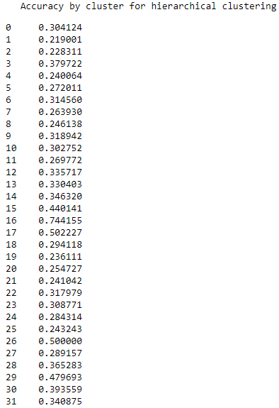
Figure 6-14. Accuracy by cluster for hierarchical clustering

HDBSCAN Application

Now, let’s turn to HDBSCAN and apply this clustering algorithm to group similar borrowers in this Lending Club dataset.

Recall that HDBSCAN will group borrowers together based on how closely packed together their attributes are in a high-dimensional space. Unlike K-means or hierarchical clustering, not all the borrowers will be grouped.

Some borrowers that are very distinct from other groups of borrowers may remain ungrouped. These are outlier borrowers and are worth investigating to see if there is a good business reason that they are dissimilar from other borrowers.

It may be true that it is possible to automatically assign numerical loan grades to some groups of borrowers but other borrowers - those that are dissimilar - require a more nuanced credit-scoring approach.

Let’s see how well HDBSCAN does.

import hdbscan

min_cluster_size = 20
min_samples = 20
alpha = 1.0
cluster_selection_method = 'leaf'

hdb = hdbscan.HDBSCAN(min_cluster_size=min_cluster_size, \
    min_samples=min_samples, alpha=alpha, \
    cluster_selection_method=cluster_selection_method)

X_train_hdbscanClustered = hdb.fit_predict(X_train)
X_train_hdbscanClustered = pd.DataFrame(data= \
    X_train_hdbscanClustered, index=X_train.index, \
    columns=['cluster'])

countByCluster_hdbscan, countByLabel_hdbscan, \
    countMostFreq_hdbscan, accuracyDF_hdbscan, \
    overallAccuracy_hdbscan, accuracyByLabel_hdbscan = \
    analyzeCluster(X_train_hdbscanClustered, y_train)

Figure 6-15 shows the overall accuracy for HDBSCAN.

Figure 6-15. Overall accuracy from HDBSCAN

As seen here, the overall accuracy is approximately 32%, worse than that of either K-means or hierarchical clustering.

Figure 6-16 shows the various clusters and their cluster sizes.

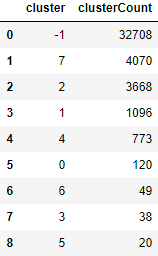
Figure 6-16. Cluster results for HDBSCAN

32,708 of the borrowers are in cluster -1, which means they are ungrouped.

Figure 6-17 shows the accuracy by cluster.

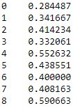
Figure 6-17. Accuracy by cluster for HDBSCAN

Among these clusters, the accuracy ranges from 28% to 59%.

Conclusion

In this chapter, we built an unsupervised clustering application based on borrowers that applied for unsecured personal loans on Lending Club from 2007-2011. The applications were based on K-means, hierarchical clustering, and hierarchical DBSCAN.

K-means performed the best, scoring an approximately 39% overall accuracy.

While these applications performed okay, they can be improved quite a bit. You should experiment with these algorithms to improve the solution from here.

This concludes the unsupervised learning using Scikit-Learn portion of the book. Next, we will explore neural network-based forms of unsupervised learning using TensorFlow and Keras.

We will start with representation learning and autoencoders in Chapter 7.