Table of Contents for
Hands-On Unsupervised Learning Using Python
 Hands-On Unsupervised Learning Using Python
Published by
O'Reilly Media, Inc., 2019
Hands-On Unsupervised Learning Using Python
Published by
O'Reilly Media, Inc., 2019
- Cover
- nav
- Hands-on Unsupervised Learning Using Python
- Hands-On Unsupervised Learning Using Python
- Preface
- I. Fundamentals of Unsupervised Learning
- 1. Unsupervised Learning in the Machine Learning Ecosystem
- 2. End-to-End Machine Learning Project
- II. Unsupervised Learning Using Scikit-Learn
- 3. Dimensionality Reduction
- 4. Anomaly Detection
- 5. Clustering
- 6. Group Segmentation
- III. Unsupervised Learning using TensorFlow and Keras
- 7. Autoencoders
- 8. Hands-On Autoencoder
- 9. Semi-Supervised Learning
- IV. Deep Unsupervised Learning using TensorFlow and Keras
- 10. Recommender Systems Using Restricted Boltzmann Machines
- 11. Feature Detection Using Deep Belief Networks
- 12. Generative Adversarial Networks
- 13. Time Series Clustering
- 14. Conclusion
- Index
- About the Author
Chapter 2. End-to-End Machine Learning Project
Before we begin exploring unsupervised learning algorithms in detail, we will review how to set up and manage machine learning projects, covering everything from acquiring data to building and evaluating a model and implementing a solution. We will work with supervised learning models in this chapter - an area most readers should have some experience in - before jumping into unsupervised learning models in the next chapter.
Environment Setup
Before we discuss the problem and explore the data, let’s set up the data science environment. This environment is the same for both supervised and unsupervised learning.
Note
These instructions are optimized for the Windows operating system but installation packages are available for Mac and Linux, too.
Version Control: Git
If you have not already, you will need to install git. Git is a version control system for coding, and all the coding examples in this book are available as Jupyter notebooks from the Git repository. Please review the git guide on how to clone repositories, add, commit, and push changes, and maintain version control by using branches.
Clone the Hands-On Unsupervised Learning Git Repository
Open the command line interface (i.e., command prompt on Windows, terminal on Mac, etc.). Navigate to the directory where you will store your unsupervised learning projects. Use the following prompt to clone the repository associated with this book from GitHub.
$ git clone https://github.com/aapatel09/handson-unsupervised-learning.git
$ git lfs pull
Alternatively, you can visit the the Git repository on the GitHub website and manually download the repository for your use. You can watch or star the repository to stay updated on changes.
Once the repository has been pulled via Git (or manually downloaded), use the command line interface to navigate into the handson-unsupervised-learning repository.
$ cd handson-unsupervised-learning
For the rest of the installations, we will continue to use the command line interface.
Scientific Libraries: Anaconda Distribution of Python
To install Python and the scientific libraries necessary for machine learning, download the Anaconda distribution of Python (version 3.6 is recommended because version 3.7 is relatively new as of the writing of this book and not supported by all the machine libraries we will use).
Create an isolated Python environment so that you can import different libraries for each project separately.
$ conda create -n unsupervisedLearning python=3.6 anaconda
This creates an isolated Python 3.6 environment - with all of the scientific libraries that come with the Anaconda distribution - called unsupervisedLearning.
Now, activate this for use.
$ activate unsupervisedLearning
Neural Networks: TensorFlow and Keras
Once unsupervisedLearning is activated, you will need to install TensorFlow and Keras to build neutral networks. TensorFlow is an open source project by Google and is not part of the Anaconda distribution.
$ pip install tensorflow
Keras is an open source netural network library that offers a higher-level API for us to use the lower-level functions in TensorFlow. In other words, we will use Keras on top of TensorFlow (the backend) to have a more intuitive set of API calls in developing our deep learning models.
$ pip install keras
Gradient Boosting, Version One: XGBoost
Next, install one version of gradient boosting known as XGBoost. To make this simple (for Windows user, at least), you can navigate into the xgboost folder in the handson-unsupervised-learning repository and find the package there.
To install the package, use pip install.
cd xgboost
pip install xgboost-0.6+20171121-cp36-cp36m-win_amd64.whl
Alternatively, download the correct version of XGBoost based on your system - either the 32-bit or the 64-bit version.
In the command line interface, navigate to the folder with this newly downloaded file.
Use pip install.
$ pip install xgboost-0.6+20171121-cp36-cp36m-win_amd64.whl
Note
Your XGBoost WHL filename may be slightly different as newer versions of the software are released publicly.
Once XGBoost has been successfully installed, navigate back to the handson-unsupervised-learning folder.
Gradient Boosting, Version Two: LightGBM
Install another version of gradient boosting, Microsoft’s LightGBM.
$ pip install lightgbm
Clustering Algorithms
Let’s install a few clustering algorithms, which we will use later in the book.
One clustering package is fastcluster, a C++ library with an interface in Python/SciPy.1
This fastcluster package can be installed with the following command in the command shell.
$ pip install fastcluster
Another is hdbscan, which can also be installed via pip.
$ pip install hdbscan
And, for time series clustering, let’s install tslearn.
$ pip install tslearn
Interactive Computing Environment: Jupyter Notebook
Jupyter notebook is part of the Anaconda distribution, so we will now activate it to launch the environment we just set up. Make sure you are in the handson-unsupervised-learning repository before you enter the following command (for ease of use).
$ jupyter notebook
You should see your browser open up and launch the http://localhost:8888/ page. Cookies must be enabled for proper access.
We are now ready to build our first machine learning project.
Overview of the Data
In this chapter, we will use a real dataset of anonymized credit card transactions made by European cardholders from September 2013.2 These transactions are labeled as fraudulent or genuine, and we will build a fraud detection solution using machine learning to predict the correct labels for never-before-seen instances.
This dataset is highly imbalanced. Of the 284,807 transactions, 492 are fraud (just 0.172%). This low percentage of fraud is pretty typical for credit card transactions.
There are 28 features, all of which are numerical. There are no categorical variables.3 These features are not the original features but rather the output of principal component analysis, which we will explore in Chapter 3. The original features were distilled to 28 principal components using this form of dimensionality reduction.
In addition to the 28 principal components, we have three other variables - the time of the transaction, the amount of the transaction, and the true class of the transaction (one if fraud, zero if genuine).
Data Preparation
Before we can use machine learning to train on the data and develop a fraud detection solution, we need to prepare the data for the algorithms.
Data Acquisition
The first step in any machine learning project is data acquisition.
Download the data
Download the dataset and, within the handson-unsupervised-learning directory, place the csv file in a folder called /datasets/credit_card_data/. If you downloaded the GitHub repository earlier, you will already have this file in this folder in the repository.
Import the necessary libraries
Import Python libraries that we will need to build our fraud detection solution.
'''Main'''importnumpyasnpimportpandasaspdimportos'''Data Viz'''importmatplotlib.pyplotaspltimportseabornassnscolor=sns.color_palette()importmatplotlibasmpl%matplotlibinline'''Data Prep'''fromsklearnimportpreprocessingasppfromscipy.statsimportpearsonrfromsklearn.model_selectionimporttrain_test_splitfromsklearn.model_selectionimportStratifiedKFoldfromsklearn.metricsimportlog_lossfromsklearn.metricsimportprecision_recall_curve,average_precision_scorefromsklearn.metricsimportroc_curve,auc,roc_auc_scorefromsklearn.metricsimportconfusion_matrix,classification_report'''Algos'''fromsklearn.linear_modelimportLogisticRegressionfromsklearn.ensembleimportRandomForestClassifierimportxgboostasxgbimportlightgbmaslgb
Read the Data
current_path=os.getcwd()file='\\datasets\\credit_card_data\\credit_card.csv'data=pd.read_csv(current_path+file)
Preview the Data
Figure 2-1 displays the first five rows of the dataset. As you can see, the data has been properly loaded.
data.head()
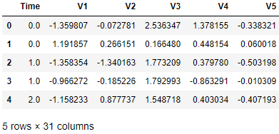
Figure 2-1. Preview of the data
Data Exploration
Next, let’s get a deeper understanding of the data. We will generate summary statistics for the data, identify any missing values or categorical features, and count the number of distinct values by feature.
Generate Summary Statistics.
Figure 2-2 describes the data, column by column. Figure 2-3 lists all the column names for easy reference. Figure 2-4 displays the total count of fraudulent transactions.
data.describe()
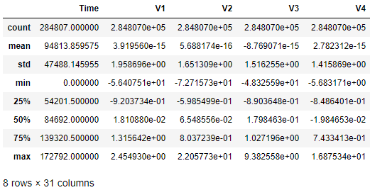
Figure 2-2. Simple summary statistics
data.columns
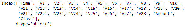
Figure 2-3. Columns in the dataset
data['Class'].sum()

Figure 2-4. The total number of positive labels
There are 284,807 instances and 31 columns as expected - 28 numerical features (V1 through V28), Time, Amount, and Class.
The timestamps range from 0 to 172,792, the amounts range from 0 to 25,691.16, and there are 492 fraudulent transactions. These fraudulent transactions are also referred to as positive cases or positive labels (labeled as one); the normal transactions are negative cases or negative labels (labeled as zero).
The 28 numerical features are not standardized yet, but we will standardize the data soon. Standardization rescales the data to have a mean of zero and standard deviation of one.
Tip
Some machine learning solutions are very sensitive to the scale of the data, so having all the data on the same relative scale - via standardization - is a good machine learning practice.
Another common method to scale data is normalization, which rescales the data to a zero to one range. Unlike the standardized data, all the normalized data is on a positive scale.
Identify non-numerical values by feature
Some machine learning algorithms cannot handle non-numerical values or missing values. Therefore, it is best practice to identify non-numerical values (also known as not a number or NaNs).
In the case of missing values, we can impute the value - for example, by replacing the missing points with the mean, median, or mode of the feature - or substitute with some user-defined value.
In the case of categorical values, we can encode the data such that all the categorical values are represented with a sparse matrix. This sparse matrix is then combined with the numerical features. The machine learning algorithm trains on this combined feature set.
Figure 2-5 shows that none of the observations have NaNs, so we will not need to impute or encode any of the values.
nanCounter=np.isnan(data).sum()
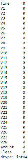
Figure 2-5. The number of NaNs by feature
Identify distinct values by feature
To develop a better understanding of the credit card transactions dataset, let’s count the number of distinct values by feature.
Figure 2-6 shoes that we have 124,592 distinct timestamps. But, from earlier, we know that we have 284,807 observations in total. That means that there are multiple transactions at some timestamps.
And, as expected, there are just two classes - one for fraud, zero for not fraud.
distinctCounter=data.apply(lambdax:len(x.unique()))
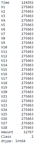
Figure 2-6. The number of distinct values by feature
Generate Feature Matrix and Labels Array
Let’s create and standardize the feature matrix X and isolate the labels array y (one for fraud, zero for not fraud). Later on we will feed these into the machine learning algorithms during training.
Create the feature matrix X and the labels array y
dataX=data.copy().drop([‘Class’],axis=1)dataY=data[‘Class’].copy()
Standardize the feature matrix X
Let’s rescale the feature matrix so that each feature, except for time, has a mean of zero and standard deviation of one.
featuresToScale=dataX.drop(['Time'],axis=1).columnssX=pp.StandardScaler(copy=True)dataX.loc[:,featuresToScale]=sX.fit_transform(dataX[featuresToScale])
As shown in Figure 2-7, the standardized features now have a mean of zero and a standard deviation of one.
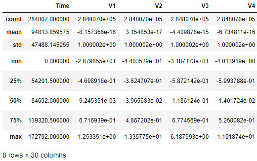
Figure 2-7. Summary of scaled features
Feature Engineering and Feature Selection
In most machine learning projects, we should consider feature engineering and feature selection as part of the solution. Feature engineering involves creating new features - for example, calculating ratios or counts or sums from the original features - to help the machine learning algorithm extract a stronger signal from the dataset.
Feature selection involves selecting a subset of the features for training, effectively removing some of the less relevant features from consideration. This may help the machine learning algorithm from overfitting to the noise in the dataset.
For this credit card fraud dataset, we do not have the original features. We have only the principal components, which were derived from PCA, a form of dimensionality reduction that we will explore in chapter three. Since we do not know what any of the features represent, we cannot perform any intelligent feature engineering.
Feature selection is not necessary either since the number of observations (284,807) vastly outnumbers the number of features (30), which dramatically reduces the chances of overfitting.
And, as Figure 2-8 shows, the features are very lowly correlated to each other. In other words, we do not have redundant features. If we did, we could remove or reduce the redundancy via dimensionality reduction.
Of course, this is not a surprise. PCA was already performed on this credit card dataset, removing the redundancy for us.
Check correlation of features
correlationMatrix=pd.DataFrame(data=[],index=dataX.columns,columns=dataX.columns)foriindataX.columns:forjindataX.columns:correlationMatrix.loc[i,j]=np.round(pearsonr(dataX.loc[:,i],dataX.loc[:,j])[0],2)
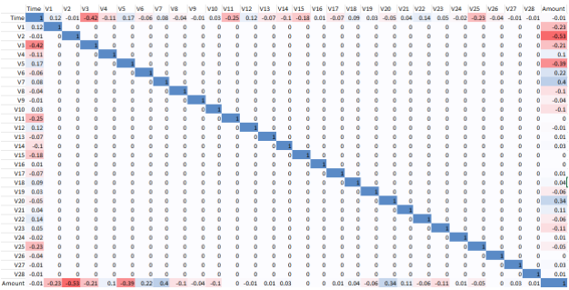
Figure 2-8. Correlation matrix
Data Visualization
As a final step, let’s visualize the data to appreciate just how imbalanced the dataset is. As Figure 2-9 shows, there are very few causes of fraud.
Since there are so few cases of fraud to learn from, this is a difficult problem to solve; fortunately, we have labels for the entire dataset.
count_classes=pd.value_counts(data['Class'],sort=True).sort_index()ax=sns.barplot(x=count_classes.index,y=tuple(count_classes/len(data)))ax.set_title('Frequency Percentage by Class')ax.set_xlabel('Class')ax.set_ylabel('Frequency Percentage')
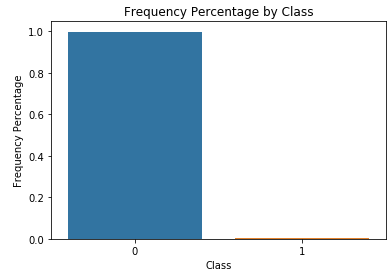
Figure 2-9. Frequency percentage of labels
Model Preparation
Now that the data is ready, let’s prepare for the model. We need to split the data into a training and a test set, select a cost function, and prepare for k-fold cross validation.
Split into Training and Test Sets
As you may recall from chapter one, machine learning algorithms learn from data (i.e., train on data) to have good performance (i.e., accurately predict) on never before seen cases. The performance on these never before seen cases is known as the generalization error - this is the most important metric in determining the goodness of a machine learning model.
We need to set up our machine learning project so that we have a training set from which the machine learning algorithm learns. We also need a test set - the never before seen cases - for which the machine learning algorithm makes predictions. The performance on this test set will be the ultimate gauge of success.
Let’s go ahead and split our credit card transactions dataset into a training set and a test set.4
X_train,X_test,y_train,y_test=train_test_split(dataX,dataY,test_size=0.33,random_state=2018,stratify=dataY)
We now have a training set with 190,280 instances (67% of the original dataset) and a test set with 93,987 instances (the remaining 33%). To preserve the percentage of fraud (~0.17%) for both the training and the test set, we have set the stratify parameter. We also fixed the random state to 2018 to make it easier to reproduce results.5
We will use the test set for a final evaluation of our generalization error (also known as out-of-sample error).
Select Cost Function
Before we train on the training set, we need a cost function (also referred to as the error rate or value function) to pass into the machine learning algorithm. The machine learning algorithm will try to minimize this cost function by learning from the training examples.
Since this is a supervised classification problem - with two classes - let’s use binary classification log loss (as shown in Figure 2-10), which will calculate the cross entropy between the true labels and the model-based predictions.6
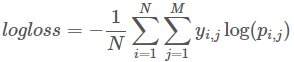
Figure 2-10. Log loss function
N is the number of observations. M is the number of class labels (here: two). Log is the natural logarithm. yi,j is 1 if observation i is in class j and 0 otherwise. pi,j is the predicted probability that observation i is in class j.
The machine learning model will generate fraud probabilities for each credit card transaction. The closer the fraud probabilities are to the true labels (i.e., one for fraud or zero for not fraud), the lower the value of the log loss function will be. This is what the machine learning algorithm will try to minimize.
Create k-Fold Cross Validation Sets
To help the machine learning algorithm estimate what its performance may be on the never before seen examples - the test set - it is best practice to further split the training set into a training set and a validation set.
For example, if we split the training set into fifths, we can train on four-fifths of the original training set and evalulate the newly training model by making predictions on the fifth slice of the original training set, known as the validation set.
It is possible to train and evaluate like this five times - leaving aside a different fifth slice as the validation set each time. This is known as k-fold cross validation, where k in this case is five.7
With this approach, we will have not one estimate but five estimates for the generalization error.
We will store the training score and the cross-validation score for each of the five runs, and we will store the cross-validation predictions each time. After all five runs are complete, we will have cross-validation predictions for the entire dataset. This will the best all-in estimate that we have for what the performance may be on the test set.
Here’s how to set up for the k-fold valiation, where k is five.
k_fold=StratifiedKFold(n_splits=5,shuffle=True,random_state=2018)
Machine Learning Models - Part One
Now we’re ready to build the machine learning models. For each machine algorithm we consider, we will set hyperparameters, train the model, and evaluate the results.
Model One - Logistic Regression
Let’s start with the most basic classification algorithm, logistic regression.8
Set hyperparameters
penalty='l2'C=1.0class_weight='balanced'random_state=2018solver='liblinear'logReg=LogisticRegression(penalty=penalty,C=C,class_weight=class_weight,random_state=random_state,solver=solver,n_jobs=n_jobs)
We will set the penalty to the default value L2 instead of L1. Compared to L1, L2 is less sensitive to outliers but will assign non-zero weights to nearly all the features, resulting in a stable solution. L1 will assign high weights to the most important features and near-zero weights to the rest, essentially performing feature selection as the algorithm trains. However, because the weights vary so much feature-to-feature, the L1 solution is not as stable to changes in data points compared to the L2 solution.9
C is the regularization strength. As you may recall from chapter one, regularization helps address overfitting by penalizing complexity. In other words, the stronger the regularization, the greater the penalty the machine learning algorithm applies to complexity. Regularization nudges the machine learning algorithm to prefer simpler models to more complex ones, all else equal.
This regularization constant, C, must be a positive floating number. The smaller the value, the stronger the regularization. We will keep the default 1.0.
Our credit card transactions dataset is very imbalanced - out of all the 284,807 cases, only 492 are fraud. As the machine learning algorithm trains, we want the algorithm to focus more attention on learning from the positive labeled transactions - in other words, the fraudulent transactions - because there are so few of them in the dataset.
For this logistic regression model, we will set the class_weight to balanced. This signals to the logistic regression algorithm that we have an imbalanced class problem; the algorithm will need to weigh the positive labels more heavily as it trains. In this case, the weights will be inversely proportional to the class frequencies; the algorithm will assign higher weights to the rare positive labels (i.e., fraud) and lower weights to the more frequent negative labels (i.e., not fraud).
The random state is fixed to 2018 to help others - such as you, the reader - reproduce results. We will keep the default solver liblinear.
Train the model
Now that the hyperparameters are set, we will train the logistic regression model on each of the five k-fold cross validation splits, training on four-fifths of the training set and evaulating the performance on the fifth slice that is held aside.
As we train and evaluate like this five times, we will calculate the cost function - log loss for our credit card transactions problem - for the training (i.e., the four-fifths slice of the original training set) and for the validation (i.e., the one-fifth slice of the original training set). We will also store the predictions for each of the five cross-validation sets; by the end of the fifth run, we will have predictions for the entire training set.
trainingScores=[]cvScores=[]predictionsBasedOnKFolds=pd.DataFrame(data=[],index=y_train.index,columns=[0,1])model=logRegfortrain_index,cv_indexink_fold.split(np.zeros(len(X_train)),y_train.ravel()):X_train_fold,X_cv_fold=X_train.iloc[train_index,:],\X_train.iloc[cv_index,:]y_train_fold,y_cv_fold=y_train.iloc[train_index],\y_train.iloc[cv_index]model.fit(X_train_fold,y_train_fold)loglossTraining=log_loss(y_train_fold,model.predict_proba(X_train_fold)[:,1])trainingScores.append(loglossTraining)predictionsBasedOnKFolds.loc[X_cv_fold.index,:]=\model.predict_proba(X_cv_fold)loglossCV=log_loss(y_cv_fold,predictionsBasedOnKFolds.loc[X_cv_fold.index,1])cvScores.append(loglossCV)('Training Log Loss: ',loglossTraining)('CV Log Loss: ',loglossCV)loglossLogisticRegression=log_loss(y_train,predictionsBasedOnKFolds.loc[:,1])('Logistic Regression Log Loss: ',loglossLogisticRegression)
Evaluate the results
For each of the five runs, we have the training log loss and the cross-validation log loss (see Figure 2-11). Generally - but not always - the training log loss will be lower than the cross-validation log loss. Because the machine learning algorithm has learned directly from the training data, its performance (i.e., its log loss) should be better on the training set than on the cross-validation set. Remember that the cross-validation set has the transactions that were explicitly held out from the training exercise.
Note
For our credit card transactions dataset, it is important to keep in mind that we are building a fraud detection solution. When we refer to the performance of the machine learning model, we mean how good is the model at predicting fraud among the transactions in the dataset.
The machine learning model outputs a prediction probability for each transaction, where one is fraud and zero is not fraud. The closer the probability is to one, the more likely the model thinks the transaction is fraudulent; the closer the probability is to zero, the more likely the model thinks the transaction is normal. By comparing the model’s probabilities with the true labels, we can assess the goodness of the model.
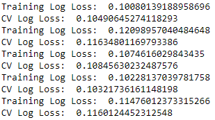
Figure 2-11. Cross-validation results of logistic regression
For each of the five runs, the training and cross-validation log losses are similar to each other. The logistic regression model does not exhibit severe overfitting; if it did, we would have a low training log loss and comparably high cross-validation log loss.
Since we stored the predictions for each of the five cross validation sets, we can combine the predictions into a single set. This single set is the same as the original training set, and we can now calculate the overall log loss for this entire training set. This is the best estimate for what the logistic regression model’s log loss will be on the test set (see Figure 2-12).

Figure 2-12. Overall log loss of logistic regression
Evaluation metrics
Although the log loss is a great all-in measure to assess the performance of the machine learning model, we may want a more intuitive way to understand the results. For example, of the fraud transactions in the training set, how many did we catch? This is known as the recall. Or, of the transactions that were flagged as fraud by the logistic regression model, how many were truly fraudulent? This is known as the precision.
Let’s introduce these and other similar evaluation metrics to help us more intuitively grasp the results.
Note
These evaluation metrics are very important because they empower data scientists to intuitively explain results to business people, who may be less familiar with log loss, cross entropy, and other cost functions. The ability to convey complex results as simply as possible to non-data scientists is an essential skill for applied data scientists.
Confusion matrix
In a typical classification problem - without class imbalance - we can evaluate the results using a confusion matrix, which is a table that summarizes the number of true positives, true negatives, false positives, and false negatives (see Figure 2-13).10
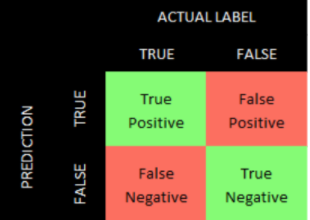
Figure 2-13. Confusion matrix
Given that our credit card transactions dataset is highly imbalanced, the confusion matrix will not be meaningful. For example, it is much easier to achieve a high number of true negatives by predicting every transaction to be negative (i.e., not fraudulent) than it is to achieve a high number of true positives because there are so few transactions are truly fraudulent.
For problems involving more balanced classes (i.e., the number of true positives is roughly similar to the number of true negatives), the confusion matrix may be a good, straightforward evaluation metric.
We need to find a more appropriate evaluation metric given our imbalanced dataset.
Precision-Recall Curve
For our imbalanced credit card transactions dataset, a better way to evaluate the results is to use precision and recall. Precision is the number of true positives over the number of total positive predictions. In other words, of all the transactions that the model predicted as fraudulent, how many are truly fraudulent?
Precision = True Positives / (True Positives + False Positives)
A high precision means that - of all our positive predictions - many are true positives (in other words, a low false positive rate).
Recall is the number of true positives over the number of total actual positives in the dataset. In other words, of all the fraudulent transactions, how many does the model catch?11
Recall = True Positives / (True Positives + False Negatives)
A high recall means that the model has captured most of the true positives (in other words, a low false negative rate).
A solution with high recall but low precision returns many results - capturing many of the positives - but most of the predictions are false alarms. A solution with high precision but low recall is the exact opposite, returning few results - capturing a fraction of all the positives in the dataset - but most of its predictions are correct.
To put this into context, if our solution had high precision but low recall, the solution would catch a very small number of the fraudulent transactions but most of the ones it would flag would be truly fraudulent.
Consider the opposite - if the solution had low precision but high recall - it would flag many of the transactions as fraudulent, thus catching a lot of the fraud, but most of the flagged transactions would be normal.
Obviously, both have major problems. In the high precision-low recall case, the credit card company would lose a lot of money due to fraud but it would not antagonize credit cardholders by unnecessarily rejecting transactions. In the low precision-high recall case, the credit card company would catch a lot of the fraud but it would most certainly anger cardholders by unnecessarily rejecting a lot of the normal, non-fraudulent transactions.
An optimal solution needs to have high precision and high recall, rejecting only those transactions that are truly fraudulent (i.e., high precision) and catching most of the fradulent cases in the dataset (high recall).
There is generally a trade-off between precision and recall, determined by the threshold set by the algorithm to separate the positive cases from the negative cases; in our example, positive is fraud and negative is not fraud. If the threshold is set too high, very few cases are predicted as positive, resulting in high precision but a low recall. As the threshold is lowered, more cases are predicted as positive, generally decreasing the precision and increasing the recall.
For our credit card transactions dataset, think of the threshold as the sensitivity of the machine learning model in rejecting transactions. If the threshold is too high/strict, the model will reject few transactions, but the ones it does reject will be very likely to be fraud.
As the threshold moves lower (i.e., becomes less strict), the model will reject more transactions, catching more of the fraudulent cases but also unnecessarily rejecting more of the normal cases as well.
A graph of the trade-off between precision and recall is known as the precision-recall curve. To evaluate the precision-recall curve, we can calculate the average precision, which is the weighted mean of the precision achieved at each threshold. The higher the average precision, the better the solution.
Note
The choice of the threshold is a very important one and usually involves the input of business decision makers. Data scientists can present the precision-recall curve to these business decision makers to figure out where the threshold should be.
For our credit card transactions dataset, the key question is how do we balance customer experience (i.e., avoid rejecting normal transactions) with fraud detection (i.e., catch the fraudulent transactions)? We cannot answer this without business input, but we will find the model with the best precision-recall curve. Then, we can present this model to business decision makers to set the appropriate threshold.
Receiver Operating Characteristic
Another good evaluation metric is the area under the receiver operating characteristic (auROC). The receiver operating characteristic (ROC) curve plots the true positive rate on the Y axis and the false positive rate on the X axis. The true positive rate can also be referred to as sensitivity, and the false positive rate can also be referred to as 1-specificity. The closer the curve is to the top left corner of the plot, the better the solution - with a value of (0.0, 1.0) as the absolute optimal point, signifying a 0% false positive rate and a 100% true positive rate.
To evaluate the solution, we can compute the area under this curve. The larger the area under the receiver operating characteristic, the better the solution.
Evaluating the logistic regression model
We have just finished introducing several evaluation metrics, including the confusion matrix, the precision-recall curve, and the receiver operating characteristic.
Let’s use these evaluation metrics to better understand the logistic regression model’s results.
First, let’s plot the precision-recall curve and calculate the average precision.
preds=pd.concat([y_train,predictionsBasedOnKFolds.loc[:,1]],axis=1)preds.columns=['trueLabel','prediction']predictionsBasedOnKFoldsLogisticRegression=preds.copy()precision,recall,thresholds=precision_recall_curve(preds['trueLabel'],preds['prediction'])average_precision=average_precision_score(preds['trueLabel'],preds['prediction'])plt.step(recall,precision,color='k',alpha=0.7,where='post')plt.fill_between(recall,precision,step='post',alpha=0.3,color='k')plt.xlabel('Recall')plt.ylabel('Precision')plt.ylim([0.0,1.05])plt.xlim([0.0,1.0])plt.title('Precision-Recall curve: Average Precision = {0:0.2f}'.format(average_precision))
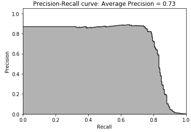
Figure 2-14. Precision-recall curve of logistic regression
Figure 2-14 is the plot of the precision-recall curve. Putting together what we discussed earlier, you can see that we can achieve approximately 80% recall (i.e., catch 80% of the fraudulent transactions) with approximately 70% precision (i.e., of the transactions the model flags as fraud, 70% are truly fraud while the remaining 30% were incorrectly flagged as fraud).
We can distill this precision-recall curve into a single number by calculating the average precision, which is 0.73 for this logistic regression model. We cannot yet tell whether this is a good or bad average precision yet since we have no other models to compare our logistic regression against.
Now, let’s measure the area under the receiver operating characteristic.
fpr,tpr,thresholds=roc_curve(preds['trueLabel'],preds['prediction'])areaUnderROC=auc(fpr,tpr)plt.figure()plt.plot(fpr,tpr,color='r',lw=2,label='ROC curve')plt.plot([0,1],[0,1],color='k',lw=2,linestyle='--')plt.xlim([0.0,1.0])plt.ylim([0.0,1.05])plt.xlabel('False Positive Rate')plt.ylabel('True Positive Rate')plt.title('Receiver operating characteristic:Areaunderthecurve={0:0.2f}'.format(areaUnderROC))plt.legend(loc="lower right")plt.show()
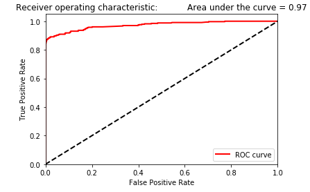
Figure 2-15. Area under the ROC curve of logistic regression
As shown in Figure 2-15, the area under the ROC curve is 0.97. This metric is just another way to evaluate the goodness of the logistic regression model, allowing you to determine how much of the fraud you can catch while keeping the false positive rate as low as possible. As with the average precision, we do not know whether this area under the ROC curve of 0.97 is good or not, but we will know more once we compare the logistic regression model’s area under the ROC curve with those of other models.
Machine Learning Models - Part Two
To compare the goodness of the logistic regression model, let’s build a few more models using other supervised learning algorithms.
Model Two - Random Forests
Let’s start with random forests.12
As with logistic regression, we will set the hyperparameters, train the model, and evaluate the results using the precision-recall curve and the area under the receiver operating characteristic curve.
Set the hyperparameters
n_estimators=10max_features='auto'max_depth=Nonemin_samples_split=2min_samples_leaf=1min_weight_fraction_leaf=0.0max_leaf_nodes=Nonebootstrap=Trueoob_score=Falsen_jobs=-1random_state=2018class_weight='balanced'RFC=RandomForestClassifier(n_estimators=n_estimators,max_features=max_features,max_depth=max_depth,min_samples_split=min_samples_split,min_samples_leaf=min_samples_leaf,min_weight_fraction_leaf=min_weight_fraction_leaf,max_leaf_nodes=max_leaf_nodes,bootstrap=bootstrap,oob_score=oob_score,n_jobs=n_jobs,random_state=random_state,class_weight=class_weight)
Let’s start with mostly default hyperparameters. The number of estimators is set at 10; in other words, we will build 10 trees and average the results across these 10 trees. For each tree, the model will consider the square root of the total number of features (in this case, the square root of 30 total features, which is 5 features, rounded down).
By setting the max_depth to none, the tree will grow as deep as possible, splitting as much as possible given the subset of features. Similar to what we did for logistic regression, we set the random state to 2018 for reproducibility of results and class weight to balanced given our imbalanced dataset.
Train the model
We will run k-fold cross validation five times, training on four-fifths of the training data and predicting on the fifth slice. We will store the predictions as we go.
trainingScores=[]cvScores=[]predictionsBasedOnKFolds=pd.DataFrame(data=[],index=y_train.index,columns=[0,1])model=RFCfortrain_index,cv_indexink_fold.split(np.zeros(len(X_train)),y_train.ravel()):X_train_fold,X_cv_fold=X_train.iloc[train_index,:],\X_train.iloc[cv_index,:]y_train_fold,y_cv_fold=y_train.iloc[train_index],\y_train.iloc[cv_index]model.fit(X_train_fold,y_train_fold)loglossTraining=log_loss(y_train_fold,\model.predict_proba(X_train_fold)[:,1])trainingScores.append(loglossTraining)predictionsBasedOnKFolds.loc[X_cv_fold.index,:]=\model.predict_proba(X_cv_fold)loglossCV=log_loss(y_cv_fold,\predictionsBasedOnKFolds.loc[X_cv_fold.index,1])cvScores.append(loglossCV)('Training Log Loss: ',loglossTraining)('CV Log Loss: ',loglossCV)loglossRandomForestsClassifier=log_loss(y_train,predictionsBasedOnKFolds.loc[:,1])('Random Forests Log Loss: ',loglossRandomForestsClassifier)
Evaluate the results
Figure 2-16 shows the training and cross-validation log loss results.
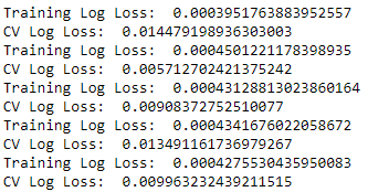
Figure 2-16. Cross-validation results of random forests
Notice that the training log losses are considerably lower than the cross-validation log losses, suggesting that the random forests classifier - with the mostly default hyperparameters - is somewhat overfitting the data during the training.

Figure 2-17. Overall log loss of random forests
Figure 2-17 shows the log loss over the entire training set (using the cross-validation predictions). Even though it is somewhat overfitting the training data, the random forests has a validation log loss that is about one-tenth that of the logistic regression - we have a significant improvement over the previous machine learning solution. The random forests model is better at correctly flagging the fraud among credit card transactions.
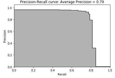
Figure 2-18. Precision-recall curve of random forests
Figure 2-18 displays the precision-recall curve. As you can see from the curve, the random forests model can catch approximately 80% of all the fraud with approximately 80% precision. This is more impressive than the approximately 80% of all the fraud the logistic regression model caught with 70% precision.
The average precision of 0.79 of the random forests model is a clear improvement over the 0.73 average precision of the logistic regression model.
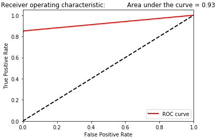
Figure 2-19. Area under the ROC curve of random forests
However, the area under the curve, shown in Figure 2-19, is somewhat worse - 0.93 for random forests versus 0.97 for logistic regression.
Model Three - Gradient Boosting Machine (XGBoost)
Now, let’s train using gradient boosting and evaluate the results. There are two popular versions of gradient boosting - one known as XGBoost and another, much faster version by Microsoft called LightGBM. Let’s build a model using each one, starting with XGBoost first.13
Set the hyperparameters
We will set this up as a binary classification problem and use log loss as the cost function. We will set the max depth of each tree to the default six and use a default learning rate of 0.3. For each tree, we will use all the observations and all the features; these are the default settings. We will set a random state of 2018 to ensure reproducibility of results.
params_xGB={'nthread':16,#number of cores'learning rate':0.3,#range 0 to 1, default 0.3'gamma':0,#range 0 to infinity, default 0# increase to reduce complexity (increase bias, reduce variance)'max_depth':6,#range 1 to infinity, default 6'min_child_weight':1,#range 0 to infinity, default 1'max_delta_step':0,#range 0 to infinity, default 0'subsample':1.0,#range 0 to 1, default 1# subsample ratio of the training examples'colsample_bytree':1.0,#range 0 to 1, default 1# subsample ratio of features'objective':'binary:logistic','num_class':1,'eval_metric':'logloss','seed':2018,'silent':1}
Train the model
As before, we will use k-fold cross-validation, training on a different four-fifths of the training data and predicting on the fifth slice for a total of five runs.
For each of the five runs, the gradient boosting model will train for as many as 2,000 rounds, evaluating whether the cross-validation log loss is decreasing as it goes. If the cross-validation log loss stops improving (over the previous 200 rounds), the training process will stop to avoid overfitting. The results of training process are very verbose, so we will not print them here but they can be found via the code on GitHub.
trainingScores=[]cvScores=[]predictionsBasedOnKFolds=pd.DataFrame(data=[],index=y_train.index,columns=['prediction'])fortrain_index,cv_indexink_fold.split(np.zeros(len(X_train)),y_train.ravel()):X_train_fold,X_cv_fold=X_train.iloc[train_index,:],\X_train.iloc[cv_index,:]y_train_fold,y_cv_fold=y_train.iloc[train_index],\y_train.iloc[cv_index]dtrain=xgb.DMatrix(data=X_train_fold,label=y_train_fold)dCV=xgb.DMatrix(data=X_cv_fold)bst=xgb.cv(params_xGB,dtrain,num_boost_round=2000,nfold=5,early_stopping_rounds=200,verbose_eval=50)best_rounds=np.argmin(bst['test-logloss-mean'])bst=xgb.train(params_xGB,dtrain,best_rounds)loglossTraining=log_loss(y_train_fold,bst.predict(dtrain))trainingScores.append(loglossTraining)predictionsBasedOnKFolds.loc[X_cv_fold.index,'prediction']=\bst.predict(dCV)loglossCV=log_loss(y_cv_fold,\predictionsBasedOnKFolds.loc[X_cv_fold.index,'prediction'])cvScores.append(loglossCV)('Training Log Loss: ',loglossTraining)('CV Log Loss: ',loglossCV)loglossXGBoostGradientBoosting=\log_loss(y_train,predictionsBasedOnKFolds.loc[:,'prediction'])('XGBoost Gradient Boosting Log Loss: ',loglossXGBoostGradientBoosting)
Evaluate the results

Figure 2-20. Overall log loss of XGBoost gradient boosting
As shown in Figure 2-20, the log loss over the entire training set (using the cross-validation predictions) is one-fifth that of the random forests and one-fiftieth that of logistic regression, representing a substantial improvement over the previous two models.
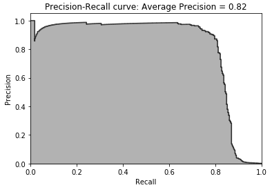
Figure 2-21. Precision-recall curve of XGBoost gradient boosting
As shown in Figure 2-21, the average precision is 0.82, just shy of that of random forests (0.79) and considerably better than that of logistic regression (0.73).
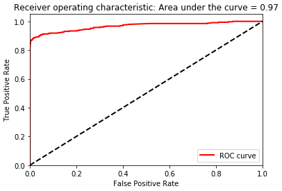
Figure 2-22. Area under the ROC curve of XGBoost gradient boosting
As shown in Figure 2-22, the area under the receiving operating characteristic curve is 0.97, same as that of logistic regression (0.97) and an improvement over random forests (0.93).
So far, gradient boosting is the best of the three models based on the log loss, the precision-recall curve, and the area under the receiving operating characteristic.
Model Four - Gradient Boosting Machine (LightGBM)
Let’s now train another version of gradient boosting known as LightGBM.14
Set the hyperparameters
We will set this up as a binary classification problem and use log loss as the cost function. We will set the max depth of each tree to 4 and use a learning rate of 0.1. For each tree, we will use all the samples and all the features; these are the default settings. We will use the default number of leaves for one tree (31) and set a random state to ensure reproducibility of results.
params_lightGB={'task':'train','application':'binary','num_class':1,'boosting':'gbdt','objective':'binary','metric':'binary_logloss','metric_freq':50,'is_training_metric':False,'max_depth':4,'num_leaves':31,'learning_rate':0.01,'feature_fraction':1.0,'bagging_fraction':1.0,'bagging_freq':0,'bagging_seed':2018,'verbose':0,'num_threads':16}
Train the model
As before, we will use k-fold cross validation and cycle through this five times, storing the predictions on the validation sets as we go.
trainingScores=[]cvScores=[]predictionsBasedOnKFolds=pd.DataFrame(data=[],index=y_train.index,columns=['prediction'])fortrain_index,cv_indexink_fold.split(np.zeros(len(X_train)),y_train.ravel()):X_train_fold,X_cv_fold=X_train.iloc[train_index,:],\X_train.iloc[cv_index,:]y_train_fold,y_cv_fold=y_train.iloc[train_index],\y_train.iloc[cv_index]lgb_train=lgb.Dataset(X_train_fold,y_train_fold)lgb_eval=lgb.Dataset(X_cv_fold,y_cv_fold,reference=lgb_train)gbm=lgb.train(params_lightGB,lgb_train,num_boost_round=2000,valid_sets=lgb_eval,early_stopping_rounds=200)loglossTraining=log_loss(y_train_fold,\gbm.predict(X_train_fold,num_iteration=gbm.best_iteration))trainingScores.append(loglossTraining)predictionsBasedOnKFolds.loc[X_cv_fold.index,'prediction']=\gbm.predict(X_cv_fold,num_iteration=gbm.best_iteration)loglossCV=log_loss(y_cv_fold,\predictionsBasedOnKFolds.loc[X_cv_fold.index,'prediction'])cvScores.append(loglossCV)('Training Log Loss: ',loglossTraining)('CV Log Loss: ',loglossCV)loglossLightGBMGradientBoosting=\log_loss(y_train,predictionsBasedOnKFolds.loc[:,'prediction'])('LightGBM Gradient Boosting Log Loss: ',loglossLightGBMGradientBoosting)
For each of the five runs, the gradient boosting model will train for as many as 2,000 rounds, evaluating whether the cross-validation log loss is decreasing as it goes. If the cross-validation log loss stops improving (over the previous 200 rounds), the training process will stop to avoid overfitting. The results of training process are very verbose, so we will not print them here but can be found via the code on GitHub.
Evaluate the results

Figure 2-23. Overall log loss of LightGBM gradient boosting
As shown in Figure 2-23, the log loss over the entire training set (using the cross-validation predictions) is similar to that of XGBoost, one-fifth that of the random forests, and one-fiftieth that of logistic regression. But, compared to XGBoost, LightGBM is considerably faster.

Figure 2-24. Precision-recall curve of LightGBM gradient boosting
As shown in Figure 2-24, the average precision is 0.82, the same as that of XGboost (0.82), better than that of random forests (0.79), and considerably better than that of logistic regression (0.73).
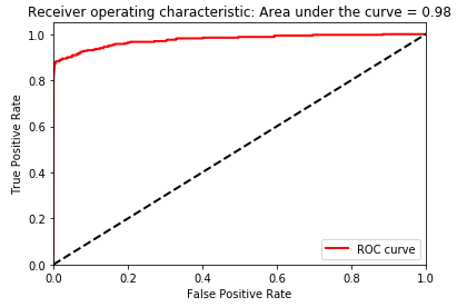
Figure 2-25. Area under the ROC curve of LightGBM gradient boosting
As shown in Figure 2-25, the area under the receiving operating characteristic curve is 0.98, an improvement over that of XGBoost (0.97), logistic regression (0.97), and random forests (0.93).
Evaluation of the Four Models Using the Test Set
So far in this chapter, we have covered how to: * Set up the environment for machine learning projects * Acquire, load, explore, clean, and visualize data * Split the dataset into training and test sets and set up k-fold cross validation sets * Choose the appropriate cost function * Set the hyperparameters and perform training and cross-validation * Evaluate the results
We have not explored how to adjust the hyperparameters (a process known as hyperparameter fine-tuning) to improve the results of each machine learning solution and address underfitting / overfitting, but the code on GitHub will allow you to conduct these experiments very easily.
Even without such fine-tuning, the results are pretty clear. Based on our training and k-fold cross-validation, LightGBM gradient boosting is the best solution, closely followed by XGBoost. Random forests and logistic regression are worse.
Let’s use the test set as a final evaluation of each of the four models that we have built.
For each model, we will use the trained model to predict the fraud probabilities for the test set transactions. Then, we will calculate the log loss for each model by comparing the fraud probabilities predicted by the model against the true fraud labels.
predictionsTestSetLogisticRegression=\pd.DataFrame(data=[],index=y_test.index,columns=['prediction'])predictionsTestSetLogisticRegression.loc[:,'prediction']=\logReg.predict_proba(X_test)[:,1]logLossTestSetLogisticRegression=\log_loss(y_test,predictionsTestSetLogisticRegression)predictionsTestSetRandomForests=\pd.DataFrame(data=[],index=y_test.index,columns=['prediction'])predictionsTestSetRandomForests.loc[:,'prediction']=\RFC.predict_proba(X_test)[:,1]logLossTestSetRandomForests=\log_loss(y_test,predictionsTestSetRandomForests)predictionsTestSetXGBoostGradientBoosting=\pd.DataFrame(data=[],index=y_test.index,columns=['prediction'])dtest=xgb.DMatrix(data=X_test)predictionsTestSetXGBoostGradientBoosting.loc[:,'prediction']=\bst.predict(dtest)logLossTestSetXGBoostGradientBoosting=\log_loss(y_test,predictionsTestSetXGBoostGradientBoosting)predictionsTestSetLightGBMGradientBoosting=\pd.DataFrame(data=[],index=y_test.index,columns=['prediction'])predictionsTestSetLightGBMGradientBoosting.loc[:,'prediction']=\gbm.predict(X_test,num_iteration=gbm.best_iteration)logLossTestSetLightGBMGradientBoosting=\log_loss(y_test,predictionsTestSetLightGBMGradientBoosting)
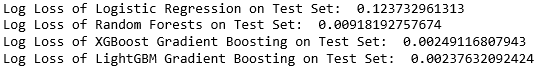
Figure 2-26. Test set scores of all four models
As shown in Figure 2-26, there are no surprises here. LightGBM Gradient Boosting has the lowest log loss on the test set, followed by the rest.
Figures 2-27 through 2-34 are the precision-recall curves, average precisions, and area under the ROC curve for all four, corroborating our findings above.
Logistic Regression
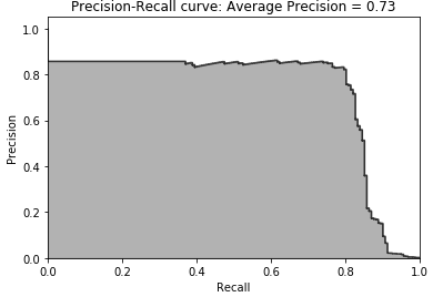
Figure 2-27. Test set precision-recall curve of logistic regression
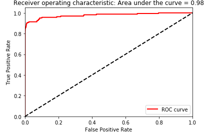
Figure 2-28. Test set area under the ROC curve of logistic regression
Random Forests
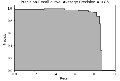
Figure 2-29. Test set precision-recall curve of random forests
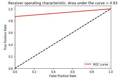
Figure 2-30. Test set area under the ROC curve of logistic regression
XGBoost Gradient Boosting
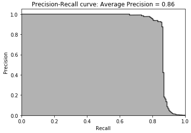
Figure 2-31. Test set precision-recall curve of XGBoost gradient boosting
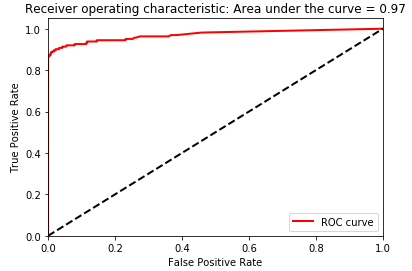
Figure 2-32. Test set area under the ROC curve of XGBoost gradient boosting
LightGBM Gradient Boosting
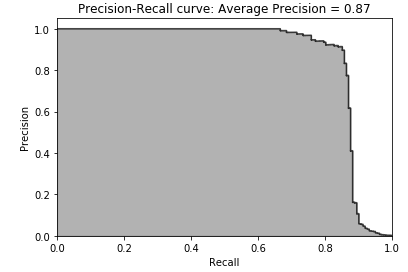
Figure 2-33. Test set precision-recall curve of LightGBM gradient boosting
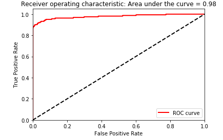
Figure 2-34. Test set area under the ROC curve of LightGBM gradient boosting
The results of LightGBM gradient boosting are impressive - we can catch over 80% of the fraudulent transactions with a nearly 90% precision (in other words, in catching 80% of the total fraud the LightGBM model gets only 10% of the cases wrong).
Considering how few cases of fraud there are in the dataset, this is a great accomplishment.
Ensembles
Instead of picking just one of the machine learning solutions we have developed for use in production, we can evaluate whether an ensemble of the models leads to an improved fraud detection rate.15
Generally, if we include similarly strong solutions from different machine learning families (such as one from random forests and one from neural networks), the ensemble of the solutions will lead to a better result than any of the standalone solutions.
This is because each of the standalone solutions has different strengths and weaknesses - by including the standalone solutions together in an ensemble, the strengths of one compensate for the weaknesses of the others, and vice versa.
There are important caveats, though. As mentioned before, each of the standalone solutions needs to be similarly strong. If one of the solutions is much better than the others, an ensemble of the bunch will not lead to improved performance. The strong solution will determine all the predictions of the ensemble.
Also, the standalone solutions need to be relatively uncorrelated. If they are very correlated, the strengths of one will mirror those of the rest, and same with the weaknesses. We will see little benefit from diversifying via an ensemble.
Stacking
In our problem here, two of the models (LightGBM Gradient Boosting and XGBoost Gradient Boosting) are much stronger than the others (Random Forests and Logistic Regression). But, the two strongest models are from the same family, which is a concern because their strengths and weaknesses will be highly correlated.
We can try stacking - a form of ensembling - to see if we see an improvement in performance compared to the standalone models from earlier. In stacking, we take the predictions from the k-fold cross-validation from each of the four standalone models (known as layer one predictions) and append them to the original training dataset. We then train on this original features plus layer one predictions dataset using k-fold cross validation.
This will result in a new set of k-fold cross-validations predictions, known as layer two predictions, which we will evaluate to see if we have an improvement in performance over any of the standalone models from earlier.
Combine layer one predictions with the original training dataset
First, let’s combine the predictions from each of the four machine learning models that we have built with the original training dataset.
predictionsBasedOnKFoldsFourModels=pd.DataFrame(data=[],index=y_train.index)predictionsBasedOnKFoldsFourModels=predictionsBasedOnKFoldsFourModels.join(predictionsBasedOnKFoldsLogisticRegression['prediction'].astype(float),\how='left').join(predictionsBasedOnKFoldsRandomForests['prediction']\.astype(float),how='left',rsuffix="2").join(\predictionsBasedOnKFoldsXGBoostGradientBoosting['prediction'].astype(float),\how='left',rsuffix="3").join(\predictionsBasedOnKFoldsLightGBMGradientBoosting['prediction'].astype(float),\how='left',rsuffix="4")predictionsBasedOnKFoldsFourModels.columns=\['predsLR','predsRF','predsXGB','predsLightGBM']X_trainWithPredictions=\X_train.merge(predictionsBasedOnKFoldsFourModels,left_index=True,right_index=True)
Set the hyperparameters
Now, we will use LightGBM Gradient Boosting - the best machine learning algorithm from the earlier exercise - to train on this original features plus layer one predictions dataset. The hyperparameters will remain the same as before.
params_lightGB={'task':'train','application':'binary','num_class':1,'boosting':'gbdt','objective':'binary','metric':'binary_logloss','metric_freq':50,'is_training_metric':False,'max_depth':4,'num_leaves':31,'learning_rate':0.01,'feature_fraction':1.0,'bagging_fraction':1.0,'bagging_freq':0,'bagging_seed':2018,'verbose':0,'num_threads':16}
Train the model
As before, we will use k-fold cross validation and generate fraud probabilities for the five different cross validation sets.
trainingScores=[]cvScores=[]predictionsBasedOnKFoldsEnsemble=\pd.DataFrame(data=[],index=y_train.index,columns=['prediction'])fortrain_index,cv_indexink_fold.split(np.zeros(len(X_train)),\y_train.ravel()):X_train_fold,X_cv_fold=\X_trainWithPredictions.iloc[train_index,:],\X_trainWithPredictions.iloc[cv_index,:]y_train_fold,y_cv_fold=y_train.iloc[train_index],y_train.iloc[cv_index]lgb_train=lgb.Dataset(X_train_fold,y_train_fold)lgb_eval=lgb.Dataset(X_cv_fold,y_cv_fold,reference=lgb_train)gbm=lgb.train(params_lightGB,lgb_train,num_boost_round=2000,valid_sets=lgb_eval,early_stopping_rounds=200)loglossTraining=log_loss(y_train_fold,\gbm.predict(X_train_fold,num_iteration=gbm.best_iteration))trainingScores.append(loglossTraining)predictionsBasedOnKFoldsEnsemble.loc[X_cv_fold.index,'prediction']=\gbm.predict(X_cv_fold,num_iteration=gbm.best_iteration)loglossCV=log_loss(y_cv_fold,\predictionsBasedOnKFoldsEnsemble.loc[X_cv_fold.index,'prediction'])cvScores.append(loglossCV)('Training Log Loss: ',loglossTraining)('CV Log Loss: ',loglossCV)loglossEnsemble=log_loss(y_train,\predictionsBasedOnKFoldsEnsemble.loc[:,'prediction'])('Ensemble Log Loss: ',loglossEnsemble)
Evaluate the results
As shown in Figure 2-35, the ensemble log loss is very similar to the standalone gradient boosting log loss - we do not see an improvement. Since the best standalone solutions are from the same family (gradient boosting), we do not see an improvement in results since they have highly correlated strengths and weaknesses in detecting fraud. There is no benefit from diversifying across models because the best models are basically the same.

Figure 2-35. Overall log loss of the ensemble
As shown in figures 2-36 and 2-37, the precision-recall curve, the average precision, and the area under the receiver operating characteristic also corroborate the lack of improvement.
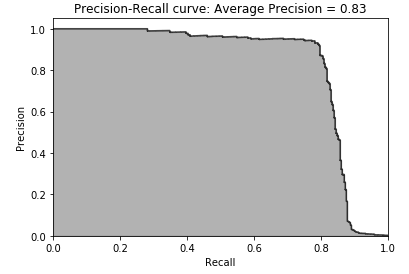
Figure 2-36. Precision-recall curve of the ensemble
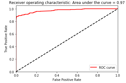
Figure 2-37. Area under the ROC curve of the ensemble
Final Model Selection
Since the ensemble does not improve performance, we favor the simplicity of the standalone LightGBM Gradient Boosting model. This is what we will use in production.
Before we create a pipeline for new, incoming transactions, let’s visualize how well the LightGBM model separates the fraudulent transactions from the normal transactions for the test set.
Figure 2-38 displays the predicted probabilities on the x-axis - blues for negative (‘0’) and oranges for positive (‘1’). Based on this plot, the model does a reasonably good job of assigning a high probability of fraud to the ones that are actually true fraud. Vice versa, the model generally assigns a low probability to the ones that are not fraud. Occasionally, the model is wrong, assigning a low probability to a case of actual fraud and a high probability to a case of not fraud.
Overall, the results are pretty impressive.
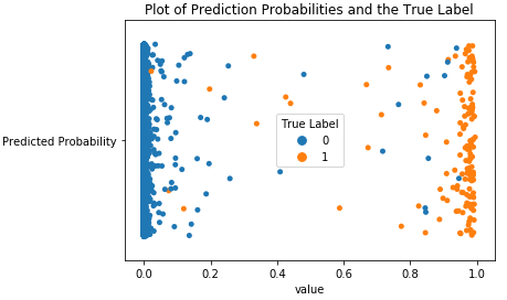
Figure 2-38. Plot of prediction probabilities and the true label
Production Pipeline
Now that we have selected a model for production, let’s design a simple pipeline that performs three simple steps on new, incoming data: load the data, scale the features, and generate predictions using the LightGBM model we have already trained and selected for use in production.
'''Pipeline for New Data'''# first, import new data into a dataframe called 'newData'# second, scale data# newData.loc[:,featuresToScale] = sX.transform(newData[featuresToScale])# third, predict using LightGBM# gbm.predict(newData, num_iteration=gbm.best_iteration)
Once these predictions are generated, analysts can act on (i.e., investigate further) the ones with the highest predicted probability of being fraud and work through the list. Or, if automation is the goal, we can have a system that automatically rejects transactions that have a predicted probability of being fraud above a certain threshold.
For example, based on the Figure 2-28, if we automatically reject transactions with a predicted probability above 0.90, we will reject cases that are almost certain to be fraud without accidentally rejecting a case of not fraud.
Conclusion
Congratulations! You have built a credit card fraud detection using supervised learning.
Together, we set up a machine learning environment, acquired and prepared the data, trained and evaluated multiple models, selected the final model for production, and designed a pipeline for new, incoming transactions. You have successfully created an applied machine learning solution.
Now, we will use this same hands-on approach to develop applied machine learning solutions using unsupervised learning.
Note
The solution above will need to be re-trained over time as the patterns of fraud change. Also, we should find other machine learning algorithms - from different machine learning families - that perform just as well as gradient boosting and include them in an ensemble to improve overall the fraud detection performance.
Finally, interpretability is very important for real world applications of machine learning. Because the features in this credit card transactions dataset are the output of principal component analysis - a form of dimensionality reduction that we will explore in the next chapter - we cannot explain in plain English why certain transactions are being flagged as potentially fraudulent. For greater interpretability of the results, we need access to the original pre-PCA features, which we do not have for this sample dataset.
1 For more on fastcluster.
2 This dataset is available via Kaggle and was collected during a research collaboration by Worldline and the Machine Learning Group of Universite Libre de Bruxelles. For more, please see Andrea Dal Pozzolo, Olivier Caelen, Reid A. Johnson and Gianluca Bontempi. Calibrating Probability with Undersampling for Unbalanced Classification. In Symposium on Computational Intelligence and Data Mining (CIDM), IEEE, 2015.
3 Categorical variables take on one of a limited number of possible qualitative values and often have to be encoded for use in machine learning algorithms.
4 For more on splitting into train and test sets.
5 For more on how the stratify parameter preserves the ratio of positive labels, please visit the official website. To reproduce the same split in your experiments, set the random state to 2018. If you set this to another number or don’t set it at all, the results will be different.
7 For more on k-fold cross validation.
8 For more on logistic regression.
9 For more on L1 versus L2.
10 True positives are instances where the prediction and the actual label are both true. True negatives are instances where the prediction and the actual label are both false. False positives are instances where the prediction is true but the actual label is false (also known as false alarm or Type I error). False negatives are instances where the prediction is false but the actual label is true (also known as miss or Type II error).
11 Recall is also known as sensitivity or true positive rate. Related to sensitivity is a concept called specificity, or the true negative rate. This is defined as the number of true negatives over the total number of total actual negatives in the dataset. Specificity = true negative rate = true negatives / (true negatives + false positives.
12 For more on random forests.
13 For more on XGBoost gradient boosting.
14 For more on Microsoft’s LightGBM gradient boosting.
15 For more on ensemble learning, please refer to these articles: resource one, resource two, and resource three.