Data Preparation

As before, let’s load in the necessary libraries and prepare the data. This should be pretty familiar by now.

'''Main'''
import numpy as np
import pandas as pd
import os, time, re
import pickle, gzip

'''Data Viz'''
import matplotlib.pyplot as plt
import seaborn as sns
color = sns.color_palette()
import matplotlib as mpl

%matplotlib inline

'''Data Prep and Model Evaluation'''
from sklearn import preprocessing as pp
from sklearn.model_selection import train_test_split
from sklearn.model_selection import StratifiedKFold
from sklearn.metrics import log_loss
from sklearn.metrics import precision_recall_curve, average_precision_score
from sklearn.metrics import roc_curve, auc, roc_auc_score

'''Algos'''
import lightgbm as lgb

'''TensorFlow and Keras'''
import tensorflow as tf
import keras
from keras import backend as K
from keras.models import Sequential, Model
from keras.layers import Activation, Dense, Dropout
from keras.layers import BatchNormalization, Input, Lambda
from keras import regularizers
from keras.losses import mse, binary_crossentropy

As before, we will generate a training and test set. But, we will drop 90% of the fraudulent credit card transactions from the training set to simulate how to work with partially labeled datasets.

While this may seem like a very aggressive move, real world problems involving payment fraud have similarly low incidences of fraud - as little as 1 fraud per 10,000 cases. By removing 90% of the labels from the training set, we are simulating this type of phenomenon.

# Load the data
current_path = os.getcwd()
file = '\\datasets\\credit_card_data\\credit_card.csv'
data = pd.read_csv(current_path + file)

dataX = data.copy().drop(['Class','Time'],axis=1)
dataY = data['Class'].copy()

# Scale data
featuresToScale = dataX.columns
sX = pp.StandardScaler(copy=True, with_mean=True, with_std=True)
dataX.loc[:,featuresToScale] = sX.fit_transform(dataX[featuresToScale])

# Split into train and test
X_train, X_test, y_train, y_test = \
    train_test_split(dataX, dataY, test_size=0.33, \
                     random_state=2018, stratify=dataY)

# Drop 95% of the labels from the training set
toDrop = y_train[y_train==1].sample(frac=0.90,random_state=2018)
X_train.drop(labels=toDrop.index,inplace=True)
y_train.drop(labels=toDrop.index,inplace=True)

We will also re-use the anomalyScores and plotResults functions.

def anomalyScores(originalDF, reducedDF):
    loss = np.sum((np.array(originalDF) - \
                   np.array(reducedDF))**2, axis=1)
    loss = pd.Series(data=loss,index=originalDF.index)
    loss = (loss-np.min(loss))/(np.max(loss)-np.min(loss))
    return loss

def plotResults(trueLabels, anomalyScores, returnPreds = False):
    preds = pd.concat([trueLabels, anomalyScores], axis=1)
    preds.columns = ['trueLabel', 'anomalyScore']
    precision, recall, thresholds = \
        precision_recall_curve(preds['trueLabel'], \
                               preds['anomalyScore'])
    average_precision = average_precision_score( \
                        preds['trueLabel'], preds['anomalyScore'])

    plt.step(recall, precision, color='k', alpha=0.7, where='post')
    plt.fill_between(recall, precision, step='post', alpha=0.3, color='k')

    plt.xlabel('Recall')
    plt.ylabel('Precision')
    plt.ylim([0.0, 1.05])
    plt.xlim([0.0, 1.0])

    plt.title('Precision-Recall curve: Average Precision = \
        {0:0.2f}'.format(average_precision))

    fpr, tpr, thresholds = roc_curve(preds['trueLabel'], \
                                     preds['anomalyScore'])
    areaUnderROC = auc(fpr, tpr)

    plt.figure()
    plt.plot(fpr, tpr, color='r', lw=2, label='ROC curve')
    plt.plot([0, 1], [0, 1], color='k', lw=2, linestyle='--')
    plt.xlim([0.0, 1.0])
    plt.ylim([0.0, 1.05])
    plt.xlabel('False Positive Rate')
    plt.ylabel('True Positive Rate')
    plt.title('Receiver operating characteristic: Area under the \
        curve = {0:0.2f}'.format(areaUnderROC))
    plt.legend(loc="lower right")
    plt.show()

    if returnPreds==True:
        return preds, average_precision

Finally, here’s a new function called precisionAnalysis to help us assess the precision of our models at a certain level of recall. Specifically, we will determine what the model’s precision is to catch 75% of the fraudulent credit card transactions in the test set. The higher the precision, the better the model.

This is a reasonable benchmark. In other words, we want to catch 75% of the fraud with as high of a precision as possible. If we do not achieve a high enough precision, we will unnecessarily reject good credit card transactions, potentially angering our customer base.

def precisionAnalysis(df, column, threshold):
    df.sort_values(by=column, ascending=False, inplace=True)
    threshold_value = threshold*df.trueLabel.sum()
    i = 0
    j = 0
    while i < threshold_value+1:
        if df.iloc[j]["trueLabel"]==1:
            i += 1
        j += 1
    return df, i/j

Supervised Model

To benchmark our semi-supervised model, let’s first see how well a supervised model and a unsupervised model do in isolation.

We will start with a supervised learning solution based on light gradient boosting like the one that performed best in chapter two.

We will use k-fold cross validation to create five folds.

k_fold = StratifiedKFold(n_splits=5,shuffle=True,random_state=2018)

Let’s next set the parameters for gradient boosting.

params_lightGB = {
    'task': 'train',
    'application':'binary',
    'num_class':1,
    'boosting': 'gbdt',
    'objective': 'binary',
    'metric': 'binary_logloss',
    'metric_freq':50,
    'is_training_metric':False,
    'max_depth':4,
    'num_leaves': 31,
    'learning_rate': 0.01,
    'feature_fraction': 1.0,
    'bagging_fraction': 1.0,
    'bagging_freq': 0,
    'bagging_seed': 2018,
    'verbose': 0,
    'num_threads':16
}

Now, let’s train the algorithm.

trainingScores = []
cvScores = []
predictionsBasedOnKFolds = pd.DataFrame(data=[], index=y_train.index, \
                                        columns=['prediction'])

for train_index, cv_index in k_fold.split(np.zeros(len(X_train)), \
                                          y_train.ravel()):
    X_train_fold, X_cv_fold = X_train.iloc[train_index,:], \
        X_train.iloc[cv_index,:]
    y_train_fold, y_cv_fold = y_train.iloc[train_index], \
        y_train.iloc[cv_index]

    lgb_train = lgb.Dataset(X_train_fold, y_train_fold)
    lgb_eval = lgb.Dataset(X_cv_fold, y_cv_fold, reference=lgb_train)
    gbm = lgb.train(params_lightGB, lgb_train, num_boost_round=2000,
                   valid_sets=lgb_eval, early_stopping_rounds=200)

    loglossTraining = log_loss(y_train_fold, gbm.predict(X_train_fold, \
                                num_iteration=gbm.best_iteration))
    trainingScores.append(loglossTraining)

    predictionsBasedOnKFolds.loc[X_cv_fold.index,'prediction'] = \
        gbm.predict(X_cv_fold, num_iteration=gbm.best_iteration)
    loglossCV = log_loss(y_cv_fold, \
        predictionsBasedOnKFolds.loc[X_cv_fold.index,'prediction'])
    cvScores.append(loglossCV)

    print('Training Log Loss: ', loglossTraining)
    print('CV Log Loss: ', loglossCV)

loglossLightGBMGradientBoosting = log_loss(y_train, \
        predictionsBasedOnKFolds.loc[:,'prediction'])
print('LightGBM Gradient Boosting Log Loss: ', \
        loglossLightGBMGradientBoosting)

We will now use this model to predict the fraud on the test set of credit card transactions.

Figure 9-1 displays the results.

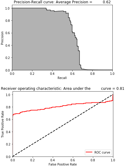
Figure 9-1. Results of supervised model

The average precision on the test based on the precision-recall curve is 0.62. To catch 75% of the fraud, we have a precision of just 0.5%.

Unsupervised Model

Now, let’s build a fraud detection solution using unsupervised learning. Specifically, we will build a sparse two-layer overcomplete autoencoder with a linear activation function. We will have 40 nodes in the hidden layer and dropout of 2%.

However, we will adjust our training set by oversampling the number of fraudulent cases we have. Oversampling is a technique to adjust the class distribution in a given data set. We want to add more fraudulent cases to our data set so that the autoencoder we train has an easier time separating the normal/non-fraudulent transactions from the abnormal/fradulent ones.

Recall that after having dropped 90% of the fraudulent cases from the training set, we have just 33 fraudulent cases left. We will take the 33 fraudulent cases, duplicate these 100 times, and append then them to the training set.

We will keep copies of the non-oversampled training set, too, so we can use them for the rest of our machine learning pipeline.

Remember we do not touch the test set - there is no oversampling with the test set, just the training set.

oversample_multiplier = 100

X_train_original = X_train.copy()
y_train_original = y_train.copy()
X_test_original = X_test.copy()
y_test_original = y_test.copy()

X_train_oversampled = X_train.copy()
y_train_oversampled = y_train.copy()
X_train_oversampled = X_train_oversampled.append( \
        [X_train_oversampled[y_train==1]]*oversample_multiplier, \
        ignore_index=False)
y_train_oversampled = y_train_oversampled.append( \
        [y_train_oversampled[y_train==1]]*oversample_multiplier, \
        ignore_index=False)

X_train = X_train_oversampled.copy()
y_train = y_train_oversampled.copy()

Let’s now train our autoencoder.

model = Sequential()
model.add(Dense(units=40, activation='linear', \
                activity_regularizer=regularizers.l1(10e-5), \
                input_dim=29,name='hidden_layer'))
model.add(Dropout(0.02))
model.add(Dense(units=29, activation='linear'))

model.compile(optimizer='adam',
              loss='mean_squared_error',
              metrics=['accuracy'])

num_epochs = 5
batch_size = 32

history = model.fit(x=X_train, y=X_train,
                    epochs=num_epochs,
                    batch_size=batch_size,
                    shuffle=True,
                    validation_split=0.20,
                    verbose=1)

predictions = model.predict(X_test, verbose=1)
anomalyScoresAE = anomalyScores(X_test, predictions)
preds, average_precision = plotResults(y_test, anomalyScoresAE, True)

Figure 9-2 displays the results.

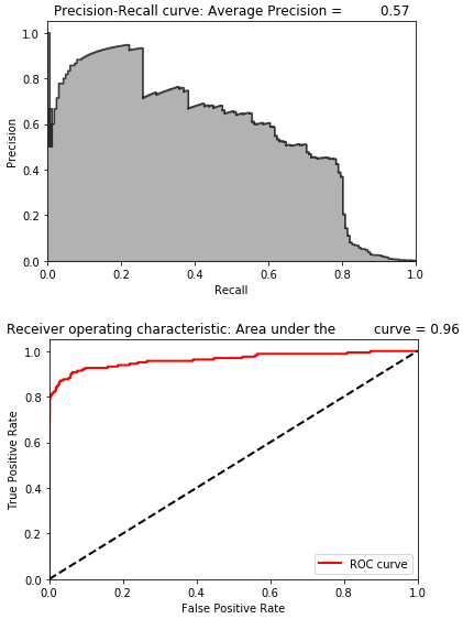
Figure 9-2. Results of unsupervised model

The average precision on the test based on the precision-recall curve is 0.57. To catch 75% of the fraud, we have a precision of just 45%.

While the average precision of the unsupervised solution is similar to the average precision of the supervised solution, the precision of 45% at 75% recall is better.

However, the unsupervised solution by itself is still not great.

Semi-Supervised Model

Now, let’s take the representation learned by autoencoder - the hidden layer - combine it with the original training set and feed this into the gradient boosting algorithm. This a semi-supervised approach, taking advantage of supervised and unsupervised learning.

To get the hidden layer, we call the Model() class from the Keras API and use the get_layer function.

layer_name = 'hidden_layer'

intermediate_layer_model = Model(inputs=model.input, \
                                 outputs=model.get_layer(layer_name).output)
intermediate_output_train = intermediate_layer_model.predict(X_train_original)
intermediate_output_test = intermediate_layer_model.predict(X_test_original)

Let’s store these autoencoder representations into DataFrames and then combine them with the original training set.

intermediate_output_trainDF = \
    pd.DataFrame(data=intermediate_output_train,index=X_train_original.index)
intermediate_output_testDF = \
    pd.DataFrame(data=intermediate_output_test,index=X_test_original.index)

X_train = X_train_original.merge(intermediate_output_trainDF, \
                                 left_index=True,right_index=True)
X_test = X_test_original.merge(intermediate_output_testDF, \
                               left_index=True,right_index=True)
y_train = y_train_original.copy()

We will now train the gradient boosting model on this new training set of 69 features (29 from the original data set and 40 from the autoencoder’s representation).

trainingScores = []
cvScores = []
predictionsBasedOnKFolds = pd.DataFrame(data=[],index=y_train.index, \
                                        columns=['prediction'])

for train_index, cv_index in k_fold.split(np.zeros(len(X_train)), \
                                          y_train.ravel()):
    X_train_fold, X_cv_fold = X_train.iloc[train_index,:], \
        X_train.iloc[cv_index,:]
    y_train_fold, y_cv_fold = y_train.iloc[train_index], \
        y_train.iloc[cv_index]

    lgb_train = lgb.Dataset(X_train_fold, y_train_fold)
    lgb_eval = lgb.Dataset(X_cv_fold, y_cv_fold, reference=lgb_train)
    gbm = lgb.train(params_lightGB, lgb_train, num_boost_round=5000,
                   valid_sets=lgb_eval, early_stopping_rounds=200)

    loglossTraining = log_loss(y_train_fold,
                                gbm.predict(X_train_fold, \
                                num_iteration=gbm.best_iteration))
    trainingScores.append(loglossTraining)

    predictionsBasedOnKFolds.loc[X_cv_fold.index,'prediction'] = \
        gbm.predict(X_cv_fold, num_iteration=gbm.best_iteration)
    loglossCV = log_loss(y_cv_fold, \
            predictionsBasedOnKFolds.loc[X_cv_fold.index,'prediction'])
    cvScores.append(loglossCV)

    print('Training Log Loss: ', loglossTraining)
    print('CV Log Loss: ', loglossCV)

loglossLightGBMGradientBoosting = log_loss(y_train, \
                        predictionsBasedOnKFolds.loc[:,'prediction'])
print('LightGBM Gradient Boosting Log Loss: ', \
                        loglossLightGBMGradientBoosting)

Figure 9-3 displays the results.

Figure 9-3. Results of semi-supervised model

The average precision on the test set based on the precision-recall curve is 0.78. This is a good bit higher than both the supervised and the unsupervised models.

To catch 75% of the fraud, we have a precision of 92%. This is a considerable improvement. With this level of precision, the payment processor should feel comfortable rejecting transactions that the model flags as potentially fraudulent. Less than one in ten will be wrong, and we will catch approximately 75% of the fraud.

The Power of Supervised and Unsupervised

In this semi-supervised credit card fraud detection solution, both supervised learning and unsupervised learning have important roles to play.

One way to explore this is by analyzing which features the final gradient boosting model found to be most important.

Let’s find and store those feature importance values from the model we just trained.

featuresImportance = pd.DataFrame(data=list(gbm.feature_importance()), \
                        index=X_train.columns,columns=['featImportance'])
featuresImportance = featuresImportance/featuresImportance.sum()
featuresImportance.sort_values(by='featImportance', \
                               ascending=False,inplace=True)
featuresImportance

Figure 9-4 shows some of the most important features, sorted in descending order.

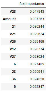
Figure 9-4. Feature importance from semi-supervised model

As you see here, some of the top featuers are features from the hidden layer learned by the autoencoder (the non “V” features) while others are the principal components from the original dataset (the “V” features) as well as the amount of the transaction.

Conclusion

The semi-supervised model trounces the performance of both the standalone supervised model and the standalone unsupervised model.

We just scratched the surface of what’s possible with semi-supervised learning, but this should help re-frame the conversation from debating between supervised and unsupervised learning to combining supervised and unsupervised learning in the search for an optimal applied solution.