Data Preparation

Let’s first load the necessary libaries.

'''Main'''
import numpy as np
import pandas as pd
import os, time, re
import pickle, gzip

'''Data Viz'''
import matplotlib.pyplot as plt
import seaborn as sns
color = sns.color_palette()
import matplotlib as mpl

%matplotlib inline

'''Data Prep and Model Evaluation'''
from sklearn import preprocessing as pp
from sklearn.model_selection import train_test_split
from sklearn.model_selection import StratifiedKFold
from sklearn.metrics import log_loss
from sklearn.metrics import precision_recall_curve, average_precision_score
from sklearn.metrics import roc_curve, auc, roc_auc_score

'''Algos'''
import lightgbm as lgb

'''TensorFlow and Keras'''
import tensorflow as tf
import keras
from keras import backend as K
from keras.models import Sequential, Model
from keras.layers import Activation, Dense, Dropout
from keras.layers import BatchNormalization, Input, Lambda
from keras import regularizers
from keras.losses import mse, binary_crossentropy

Next, load the dataset and prepare it for use. We will create a dataX matrix with all the PCA components and the feature Amount. But, we will drop Class and Time.

We will store the Class labels in the dataY matrix.

We will also scale the features in the dataX matrix so that all the features have a mean of zero and standard deviation of one.

data = pd.read_csv('creditcard.csv')
dataX = data.copy().drop(['Class','Time'],axis=1)
dataY = data['Class'].copy()
featuresToScale = dataX.columns
sX = pp.StandardScaler(copy=True, with_mean=True, with_std=True)
dataX.loc[:,featuresToScale] = sX.fit_transform(dataX[featuresToScale])

As we did in Chapter 3, we will create a training set with two-thirds of the data and the labels and a test set with one-third of the data and the labels.

Let’s store the training set and the test set as X_train_AE and X_test_AE, respectively.

We will use these in the autoencoders soon.

X_train, X_test, y_train, y_test = \
    train_test_split(dataX, dataY, test_size=0.33, \
                     random_state=2018, stratify=dataY)

X_train_AE = X_train.copy()
X_test_AE = X_test.copy()

Let’s also use re-use the function we introduced earlier in the book, called anomalyScores, to calculate the reconstruction error between the original feature matrix and the newly reconstructed feature matrix. The function takes the sum of squared errors and normalizes them to a range between zero and one.

This is a crucial function. The transactions with errors close to one are the ones that are most anomalous (i.e., have the highest reconstruction error) and, therefore, are most likely to be fraudulent.

The transactions with errors close to zero have the lowest reconstruction error and are most likely to be normal.

def anomalyScores(originalDF, reducedDF):
    loss = np.sum((np.array(originalDF) - \
                   np.array(reducedDF))**2, axis=1)
    loss = pd.Series(data=loss,index=originalDF.index)
    loss = (loss-np.min(loss))/(np.max(loss)-np.min(loss))
    return loss

We will also re-use the function to plot the precision-recall curve, the average precision, and the receiver operating characteristic curve. The function is called plotResults.

def plotResults(trueLabels, anomalyScores, returnPreds = False):
    preds = pd.concat([trueLabels, anomalyScores], axis=1)
    preds.columns = ['trueLabel', 'anomalyScore']
    precision, recall, thresholds = \
        precision_recall_curve(preds['trueLabel'], \
                               preds['anomalyScore'])
    average_precision = average_precision_score( \
                        preds['trueLabel'], preds['anomalyScore'])

    plt.step(recall, precision, color='k', alpha=0.7, where='post')
    plt.fill_between(recall, precision, step='post', alpha=0.3, color='k')

    plt.xlabel('Recall')
    plt.ylabel('Precision')
    plt.ylim([0.0, 1.05])
    plt.xlim([0.0, 1.0])

    plt.title('Precision-Recall curve: Average Precision = \
        {0:0.2f}'.format(average_precision))

    fpr, tpr, thresholds = roc_curve(preds['trueLabel'], \
                                     preds['anomalyScore'])
    areaUnderROC = auc(fpr, tpr)

    plt.figure()
    plt.plot(fpr, tpr, color='r', lw=2, label='ROC curve')
    plt.plot([0, 1], [0, 1], color='k', lw=2, linestyle='--')
    plt.xlim([0.0, 1.0])
    plt.ylim([0.0, 1.05])
    plt.xlabel('False Positive Rate')
    plt.ylabel('True Positive Rate')
    plt.title('Receiver operating characteristic: Area under the \
        curve = {0:0.2f}'.format(areaUnderROC))
    plt.legend(loc="lower right")
    plt.show()

    if returnPreds==True:
        return preds

The Components of an Autoencoder

First, let’s build a very simple autoencoder with the input layer, a single hidden layer, and the output layer.

We will feed the original feature matrix x into the autoencoder - this is represented by the input layer.

Then, an activation function will be applied to the input layer, generating the hidden layer. This activation function is called f and represents the encoder portion of the autoencoder.

The hidden layer is called h (which is equal to f(x)) and represents the newly learned representation.

Next, an activation function is applied to the hidden layer (i.e., the newly learned representation) to reconstruct the original observations. This activation function is called g and represents the decoder portion of the autoencoder.

The output layer is called r (which is equal to g(h)) and represents the newly reconstructed observations.

To calculate the reconstruction error, we will compare the newly constructed observations r with the original ones x.

Activation Functions

Before we decide the number of nodes to use in this single hidden layer autoencoder, let’s discuss activation functions.

A neural network learns the weights to apply to the nodes at each of the layers but whether the nodes will be activated or not (for use in the next layer) is determined by the activation function.

In other words, an activation function is applied to the weighted input (plus bias, if any) at each layer. Let’s call the weighted input plus bias Y.

The activation function takes in Y and either activates (if Y is above a certain threshold) or does not.

If activated, the information in a given node is passed to the next layer; otherwise, it is not.

However, we do not want simple binary activations. Instead, we want a range of activation values.

To do this, we can choose a linear activation function or a non-linear activation function. Common non-linear activation functions include sigmoid, hyperbolic tangent (or tanh for short), rectified linear unit (or ReLu for short), and softmax.

The linear activation function is unbounded. It can generate activation values between negative infinity and positive infinity.

The sigmoid function is bounded and can generate activation values between zero and one.

The tanh function is also bounded and can generate activation values between negative one and positive one. Its gradient is steeper than that of the sigmoid function.

The ReLu function has an interesting property. If Y is positive, ReLu will return Y. Otherwise, it will return zero. Therefore, ReLu is unbounded for positive values of Y.

The softmax function is used as the final activation function in a neural network for classification problems because it normalizes classification probabilities to values that add up to a probability of one.

Of all these functions, the linear activation function is the simplest and least computationally expensive. ReLu is the next least computationally expensive, followed by the others.

Our First Autoencoder

Let’s start with a two-layer autoencoder with a linear activation function for both the encoder and the decoder functions. Note that only the number of hidden layers plus the output layer count towards the number of layers in a neural network. Since we have a single hidden layer, this is known as a two-layer neural network.

To build this using TensorFlow and Keras, we must first call the Sequential model API. The Sequential model is a linear stack of layers, and we will pass the types of layers we want into the model before we compile the model and train on our data.¹

# Model one
# Two layer complete autoencoder with linear activation

# Call neural network API
model = Sequential()

Once we call the Sequential model, we then need to specify the input shape by designating the number of dimensions, which should match the number of dimensions in the original feature matrix, dataX. This number is 29.

We also need to specify the activation function (also known as the encoder function) applied to the input layer and the number of nodes we want the hidden layer to have. We will pass linear as the activation function.

To start, let’s use a complete autoencoder, where the number of nodes in the hidden layer equals the number of nodes in the input layer, which is 29.

All of this is done using a single line of code.

model.add(Dense(units=29, activation='linear',input_dim=29))

Similarly, we need to specify the activation function (also known as the decoder function) applied to the hidden layer to reconstruct the observations and the number of dimensions we want the output layer to have. Since we want the final reconstructed matrix to have the same dimensions as the original matrix, the dimensions needs to be 29. And, we will use a linear activation function for the decoder, too.

model.add(Dense(units=29, activation='linear'))

Next, we will need to compile the layers we have designed for the neural network. This requires us to select a loss function (also known as the objective function) to guide the learning of the weights, an optimizer to set the process by which the weights are learned, and a list of metrics to output to help us evaluate the goodness of the neural network.

Training the Model

Finally, we need to choose the evaluation metrics, which we will set to accuracy to keep things simple.⁵

model.compile(optimizer='adam',
              loss='mean_squared_error',
              metrics=['accuracy'])

Next, we need to select the number of epochs, the batch size, and then begin the training process by calling the method fit.

The number of epochs determines the number of times the training occurs over the entire dataset we pass into the neural network. We will set this to 10 to start.

The batch sets the number of samples the neural network trains on before making the next gradient update. If the batch is equal to the total number of observations, the neural network will make a gradient update once every epoch. Otherwise, it will make updates multiple times per epoch. We will set this to a generic 32 samples to start.

Into the fit method, we will pass in the initial input matrix, x, and the target matrix, y. In our case, both x and y will be the original feature matrix, X_train_AE, because we want to compare the output of the autoencoder - the reconstructed feature matrix - with the original feature matrix to calculate reconstruction error.

Recall this is a purely unsupervised solution so we will not use the y matrix at all.

We will also validate our model as we go by testing the reconstruction error on the entire training matrix.

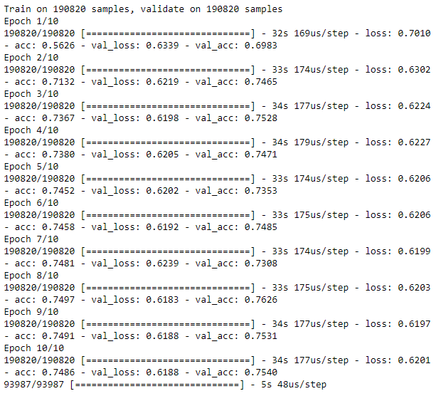
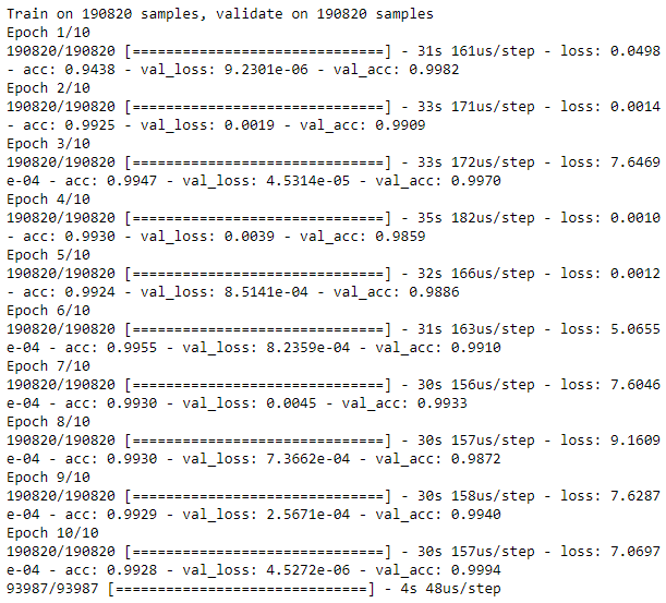
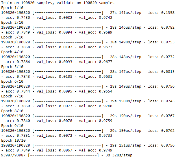
num_epochs = 10
batch_size = 32

history = model.fit(x=X_train_AE, y=X_train_AE,
                    epochs=num_epochs,
                    batch_size=batch_size,
                    shuffle=True,
                    validation_data=(X_train_AE, X_train_AE),
                    verbose=1)

Since this a complete autoencoder - where the hidden layer has the same number of dimensions as the input layer - the loss is very low, for both the training and validation sets (see Figure 8-1).

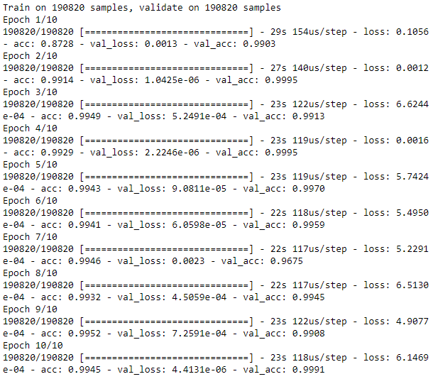
Figure 8-1. Training history of complete autoencoder

This is not optimal - the autoencoder has reconstructed the original feature matrix too precisely, memorizing the inputs.

Recall that the autoencoder is meant to learn a new representation that captures the most salient information in the original input matrix while dropping the less relevant information. Simply memorizing the inputs - also known as learning the identity function - will not result in new and improved representation learning.

Evaluating on the Test Set

Let’s use the test set to evaluate just how successively this autoencoder can identify fraud in the credit card transactions dataset. We will use the predict method to do this.

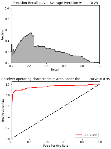
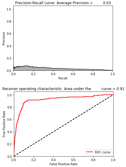
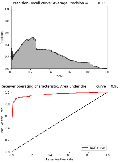
predictions = model.predict(X_test, verbose=1)
anomalyScoresAE = anomalyScores(X_test, predictions)
preds = plotResults(y_test, anomalyScoresAE, True)

As seen in Figure 8-2, the average precision is 0.30, which is not very good. The best average precision using unsupervised learning from Chapter 4 was 0.69, and the supervised system had an average precision of 0.82.

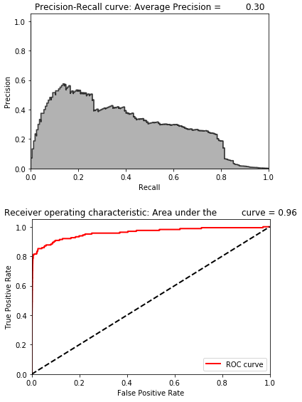
Figure 8-2. Evaluation metrics of complete autoencoder

However, each training process will yield slightly different results for the trained autoencoder, so you may not see the same performance for your run.

To get a better sense of how a two-layer complete autoencoder performs on the test set, let’s run this training process ten separate times and store the average precision on the test set for each run. We will assess how good this complete autoencoder is at capturing fraud based on the mean of the average precision from these 10 runs.

To consolidate our work thus far, here is the code to simulate 10 runs from start to finish.

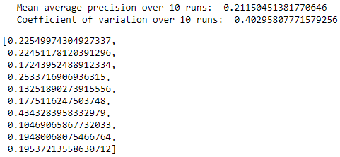
# 10 runs - We will capture mean of average precision
test_scores = []
for i in range(0,10):
    # Call neural network API
    model = Sequential()

    # Apply linear activation function to input layer
    # Generate hidden layer with 29 nodes, the same as the input layer
    model.add(Dense(units=29, activation='linear',input_dim=29))

    # Apply linear activation function to hidden layer
    # Generate output layer with 29 nodes
    model.add(Dense(units=29, activation='linear'))

    # Compile the model
    model.compile(optimizer='adam',
                  loss='mean_squared_error',
                  metrics=['accuracy'])

    # Train the model
    num_epochs = 10
    batch_size = 32

    history = model.fit(x=X_train_AE, y=X_train_AE,
                        epochs=num_epochs,
                        batch_size=batch_size,
                        shuffle=True,
                        validation_data=(X_train_AE, X_train_AE),
                        verbose=1)

    # Evaluate on test set
    predictions = model.predict(X_test, verbose=1)
    anomalyScoresAE = anomalyScores(X_test, predictions)
    preds, avgPrecision = plotResults(y_test, anomalyScoresAE, True)
    test_scores.append(avgPrecision)

print("Mean average precision over 10 runs: ", np.mean(test_scores))
test_scores

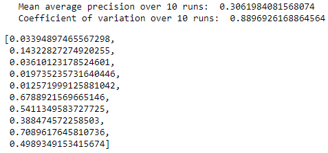
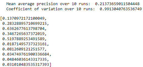
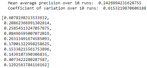
Figure 8-3 summarizes the results for the 10 runs. The mean of the average precision is 0.30, but the average precision ranges from a low of 0.02 to .72.

The coefficient of variation (defined as the standard deviation divided by the mean over 10 runs) is 0.88.

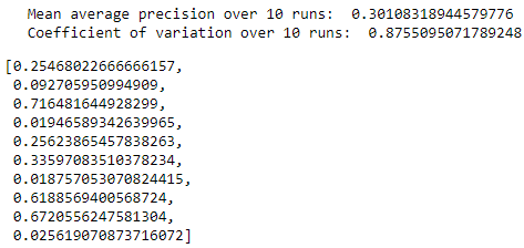
Figure 8-3. Summary over 10 runs for complete autoencoder

Let’s try to improve our results by building variations of this autoencoder.

Two-Layer Undercomplete Autoencoder with Linear Activation Function

Let’s try an undercomplete autoencoder rather than a complete one.

Compared to the previous autoencoder, the only thing that changes is the number of nodes in the hidden layer. Instead of setting this to the number of original dimensions - 29 - we will set the nodes to 20.

In other words, this autoencoder is a constrained autoencoder. The encoder function is forced to capture the information in the input layer with a fewer number of nodes, and the decoder has to take this new representation to reconstruct the original matrix.

We should expect the loss here to be higher compared to that of the complete autoencoder. Let’s run the code. We will perform ten independent runs to test how well the various undercomplete autoencoders are at catching fraud.

# 10 runs - We will capture mean of average precision
test_scores = []
for i in range(0,10):
    # Call neural network API
    model = Sequential()

    # Apply linear activation function to input layer
    # Generate hidden layer with 20 nodes
    model.add(Dense(units=20, activation='linear',input_dim=29))

    # Apply linear activation function to hidden layer
    # Generate output layer with 29 nodes
    model.add(Dense(units=29, activation='linear'))

    # Compile the model
    model.compile(optimizer='adam',
                  loss='mean_squared_error',
                  metrics=['accuracy'])

    # Train the model
    num_epochs = 10
    batch_size = 32

    history = model.fit(x=X_train_AE, y=X_train_AE,
                        epochs=num_epochs,
                        batch_size=batch_size,
                        shuffle=True,
                        validation_data=(X_train_AE, X_train_AE),
                        verbose=1)

    # Evaluate on test set
    predictions = model.predict(X_test, verbose=1)
    anomalyScoresAE = anomalyScores(X_test, predictions)
    preds, avgPrecision = plotResults(y_test, anomalyScoresAE, True)
    test_scores.append(avgPrecision)

print("Mean average precision over 10 runs: ", np.mean(test_scores))
test_scores

As Figure 8-4 shows, the losses of the undercomplete autoencoder are considerably higher than those of the complete autoencoder. It is clear that the autoencoder learns a representation that is a new and more constrained representation from the original input matrix - the autoencoder did not simply memorize the inputs.

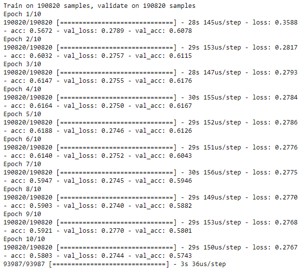
Figure 8-4. Training history of undercomplete autoencoder with 20 nodes

This is how an autoencoder should work - it should learn a new representation. Figure 8-5 shows how effective this new representation is at identifying fraud.

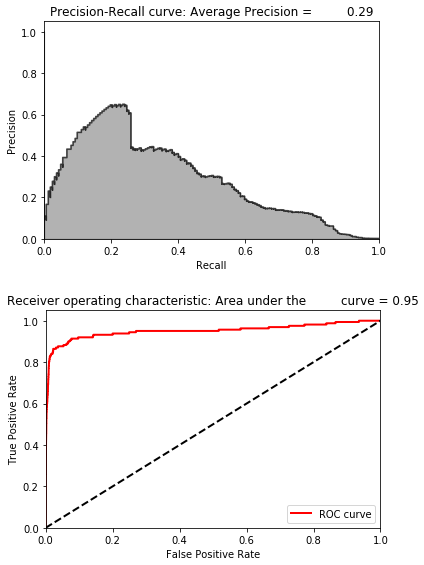
Figure 8-5. Evaluation metrics of undercomplete autoencoder with 20 nodes

The average precision is 0.29, similar to that of the complete autoencoder.

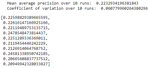
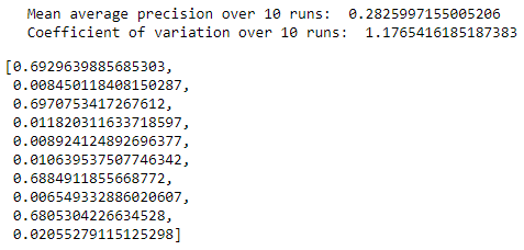
Figure 8-6 shows the distribution of average precisions across the 10 runs. The mean of the average precision is 0.31, but the dispersion of average precisions is very tight (as the coefficient of variation of 0.03 indicates). This is a considerably more stable system at catching fraud than the one designed with a complete autoencoder.

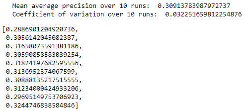
Figure 8-6. Summary over 10 runs for undercomplete autoencoder with 20 nodes

But, we are still stuck at a fairly mediocre average precision.

Why did the undercomplete autoencoder not perform better? It could be that this undercomplete autoencoder does not have enough nodes. Or, we need to train using more hidden layers. Let’s experiment with these two changes, one by one.

Increasing the Number of Nodes

Figure 8-7 displays the training losses from using a two-layer undercomplete autocoder with 27 nodes instead of just 20.

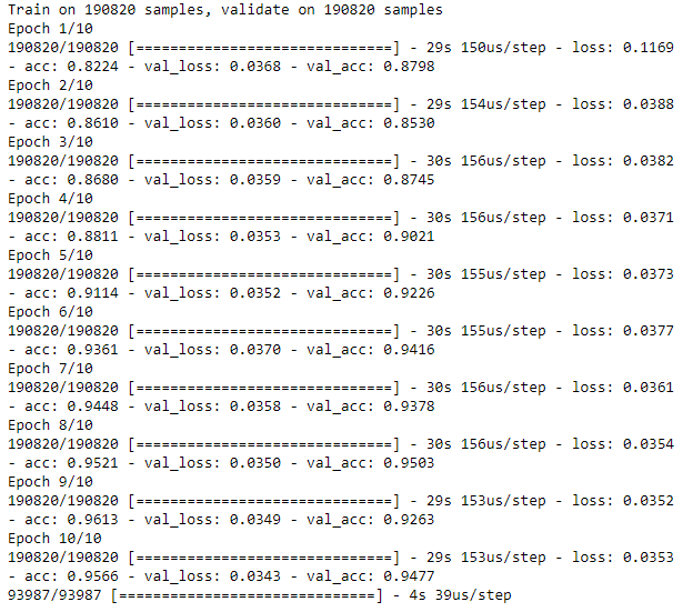
Figure 8-7. Training history of undercomplete autoencoder with 27 nodes

Figure 8-8 displays the average precision, precision-recall curve, and the area under the ROC curve.

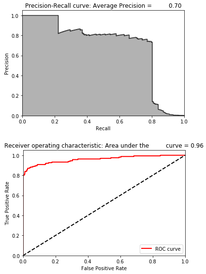
Figure 8-8. Evaluation metrics of undercomplete autoencoder with 27 nodes

The average precision improves considerably to 0.70. This is better than the average precision of the complete autoencoder and better than the best unsupervised learning solution from chapter four.

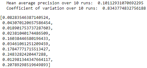
Figure 8-9 summarizes the distribution of average precisions across the 10 runs. The mean of the average precision is 0.53, considerably better than the ~0.30 average precision earlier. The dispersion of average precisions is reasonably good, with a coefficient of variation of 0.50.

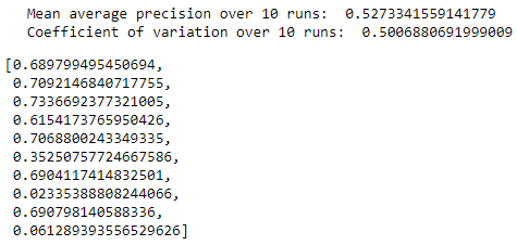
Figure 8-9. Summary over 10 runs for undercomplete autoencoder with 27 nodes

We have a clear improvement over our previous autoencoder-based anomaly detection system.

Adding More Hidden Layers

Let’s see if we can improve our results by adding an extra hidden layer to the autoencoder. We will continue to use linear activation functions for now.

Experimentation

Experimentation is a major part of discovering the best neural network architecture for the problem you have to solve. Some changes you make will lead to better results, others to worse. Knowing how to modify the neural net and the hyperparameters as part of your search to improve the solution is very important.

Instead of a single hidden layer with 27 nodes, we will use one hidden layer with 28 nodes and another with 27 nodes. This is only a slight variation from the one we used previously.

This is now a three-layer neural network since we have two hidden layers plus the output layer. The input layer does not “count” towards this number.

This additional hidden layer requires just one additional line of code, as shown here.

# Model two
# Three layer undercomplete autoencoder with linear activation
# With 28 and 27 nodes in the two hidden layers, respectively

model = Sequential()
model.add(Dense(units=28, activation='linear',input_dim=29))
model.add(Dense(units=27, activation='linear'))
model.add(Dense(units=29, activation='linear'))

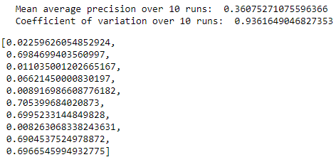
Figure 8-10 summarizes the distribution of average precisions across the 10 runs. The mean of the average precision is 0.36, worse than the 0.53 we just achieved. The dispersion of average precisions is also worse, with a coefficient of variation of 0.94 (higher is worse).

Figure 8-10. Summary over 10 runs for undercomplete autoencoder with two hidden layers

Non-Linear Autoencoder

Now let’s build an undercomplete autoencoder using a non-linear activation function. We will use ReLu, but you are welcome to experiment with tanh, sigmoid, and the other non-linear activation functions.

We will include three hidden layers, with 27, 22, and 27 nodes, respectively. Conceptually, the first two activation functions (applied on the input and first hidden layer) perform the encoding, creating the second hidden layer with 22 nodes. Then, the next two activation functions perform the decoding, reconstructing the 22-node representation to the original number of dimensions, 29.

model = Sequential()
model.add(Dense(units=27, activation='relu',input_dim=29))
model.add(Dense(units=22, activation='relu'))
model.add(Dense(units=27, activation='relu'))
model.add(Dense(units=29, activation='relu'))

Figure 8-11 shows the losses from this autoencoder, and Figure 8-12 displays the average precision, the precision-recall curve, and the area under the ROC curve.

Figure 8-11. Training history of undercomplete autoencoder with three hidden layers and ReLu activation function

Figure 8-12. Evaluation metrics of undercomplete autoencoder with three hidden layers and ReLu activation function

The results are considerably worse.

Figure 8-13 summarizes the distribution of average precisions across the 10 runs. The mean of the average precision is 0.22, worse than the 0.53 we achieved earlier. The dispersion of average precisions is very tight, with a coefficient of variation of 0.06.

Figure 8-13. Summary over 10 runs for undercomplete autoencoder with three hidden layers and ReLu activation function

These results are much worse than those from a simple autoencoder using a linear activation function. It could be that - for this dataset - a linear, undercomplete autoencoder is the best solution.

For other datasets, that may not always be the case. As always, experimentation is required to find the optimal solution. I encourage you to experiment with the code. Change the number of nodes, the number of hidden layers, and the mix of activation functions, and see how much better or worse the solutions become.

This type of experimentation is known as hyperparameter optimization. You are adjusting the hyperparameters - the number of nodes, the number of layers, and the mix of activation functions - in search of the optimal solution.

Overcomplete Autoencoder with Linear Activation

Now, let’s highlight the problem with overcomplete autoencoders. Overcomplete autoencoders have more nodes in the hidden layer than either the input or output layer. Because the capacity of the neural network model is so high, the autoencoder simply memorizes the observations it trains on.

In other words, the autoencoder learns the identity function, which is exactly what we want to avoid. The autoencoder will overfit the training data and will perform very poorly in separating fraudulent credit card transactions from normal ones.

Recall that we need the autoencoder to learn the salient aspects of the credit card transactions in the training set so that it learns what the normal transactions look like - without memorizing the information in the less normal, rare transactions of the fraudulent variety.

Only if the autoencoder is able to lose some of the information in the training set will it be able to separate the fraudulent transactions from the normal ones.

model = Sequential()
model.add(Dense(units=40, activation='linear',input_dim=29))
model.add(Dense(units=29, activation='linear'))

Figure 8-14 shows the losses from this autoencoder, and Figure 8-15 displays the average precision, the precision-recall curve, and the area under the ROC curve.

Figure 8-14. Training history of overcomplete autoencoder with single hidden layer and linear activation function

Figure 8-15. Evaluation metrics of overcomplete autoencoder with single hidden layer and linear activation function

As expected, the losses are very low, and the overfit overcomplete autoencoder has very poor performance detecting the frauduluent credit card transactions.

Figure 8-16 summarizes the distribution of average precisions across the 10 runs. The mean of the average precision is 0.31, worse than the 0.53 we achieved earlier. The dispersion of average precisions is not very tight, with a coefficient of variation of 0.89.

Figure 8-16. Summary over 10 runs for overcomplete autoencoder with single hidden layer and linear activation function

Overcomplete Autoencoder with Linear Activation and Dropout

One way to improve the overcomplete autoencoder solution is to use a regularization technique to reduce the overfitting. One such technique is known as dropout. With dropout, we force the autoencoder to drop out some defined percentage of units from the layers in the neural network.

With this new constraint, the overcomplete autoencoder cannot simply memorize the credit card transactions in the training set. Instead, the autoencoder has to generalize a bit more. The autoencoder is forced to learn more of the salient features in the dataset and lose some of the less salient information.

We will use a dropout percentage of 10%, which we will apply to the hidden layer. In other words, 10% of the neurons are dropped. The higher the dropout percentage, the stronger the regularization. This is done with just a single additional line of code.

Let’s see if this improves the results.

model = Sequential()
model.add(Dense(units=40, activation='linear', input_dim=29))
model.add(Dropout(0.10))
model.add(Dense(units=29, activation='linear'))

Figure 8-17 shows the losses from this autoencoder, and Figure 8-18 displays the average precision, the precision-recall curve, and the area under the ROC curve.

Figure 8-17. Training history of overcomplete autoencoder with single hidden layer, dropout, and linear activation function

Figure 8-18. Evaluation metrics of overcomplete autoencoder with single hidden layer, dropout, and linear activation function

As expected, the losses are very low, and the overfit overcomplete autoencoder has very poor performance detecting the frauduluent credit card transactions.

Figure 8-19 summarizes the distribution of average precisions across the 10 runs. The mean of the average precision is 0.21, worse than the 0.53 we achieved earlier. The coefficient of variation is 0.40.

Figure 8-19. Summary over 10 runs for overcomplete autoencoder with single hidden layer, dropout, and linear activation function

Sparse Overcomplete Autoencoder with Linear Activation

Another regularization technique is sparsity. We can force the autoencoder to take the sparsity of the matrix into consideration such that the majority of the autoencoder’s neurons are inactive most of the time - in other words, they do not fire.

This makes it harder for the autoencoder to memorize the identity function even when the autoencoder is overcomplete because most of the nodes cannot fire and, therefore, cannot overfit the observations as easily.

We will use a single hidden layer overcomplete autoencoder with 40 nodes like before but with just the sparsity penalty, not dropout.

Let’s see if the results improve from the 0.21 average precision we had earlier.

model = Sequential()
    model.add(Dense(units=40, activation='linear',  \
        activity_regularizer=regularizers.l1(10e-5), input_dim=29))
model.add(Dense(units=29, activation='linear'))

Figure 8-20 shows the losses from this autoencoder, and Figure 8-21 displays the average precision, the precision-recall curve, and the area under the ROC curve.

Figure 8-20. Training history of sparse overcomplete autoencoder with single hidden layer and linear activation function

Figure 8-21. Evaluation metrics of sparse overcomplete autoencoder with single hidden layer and linear activation function

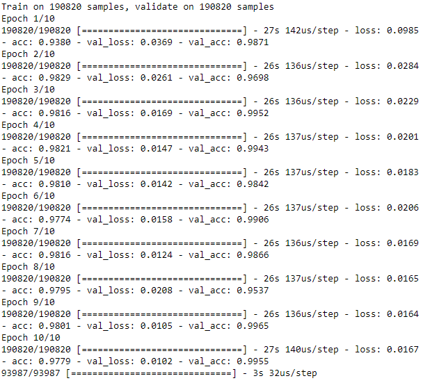
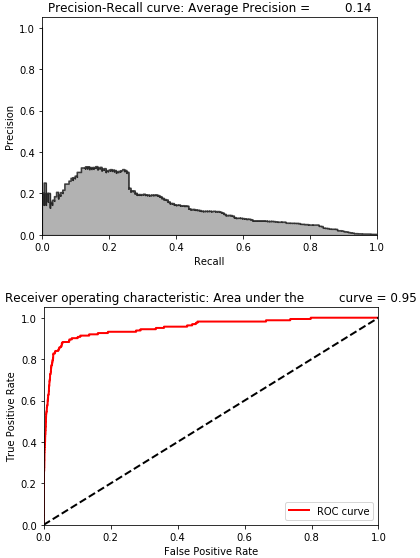
Figure 8-22 summarizes the distribution of average precisions across the 10 runs. The mean of the average precision is 0.21, worse than the 0.53 we achieved earlier. The coefficient of variation is 0.99.

Figure 8-22. Summary over 10 runs of sparse overcomplete autoencoder with single hidden layer and linear activation function

Sparse Overcomplete Autoencoder with Linear Activation and Dropout

Of course, we can combine the regularization techniques to improve the solution. Here is a sparse overcomplete autoencoder with linear activation, 40 nodes in the single hidden layer, and dropout of 5%.

model = Sequential()
    model.add(Dense(units=40, activation='linear',  \
        activity_regularizer=regularizers.l1(10e-5), input_dim=29))
    model.add(Dropout(0.05))
model.add(Dense(units=29, activation='linear'))

Figure 8-23 shows the losses from this autoencoder, and Figure 8-24 displays the average precision, the precision-recall curve, and the area under the ROC curve.

Figure 8-23. Training history of sparse overcomplete autoencoder with single hidden layer, dropout, and linear activation function

Figure 8-24. Evaluation metrics of sparse overcomplete autoencoder with single hidden layer, dropout, and linear activation function

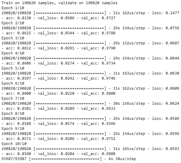
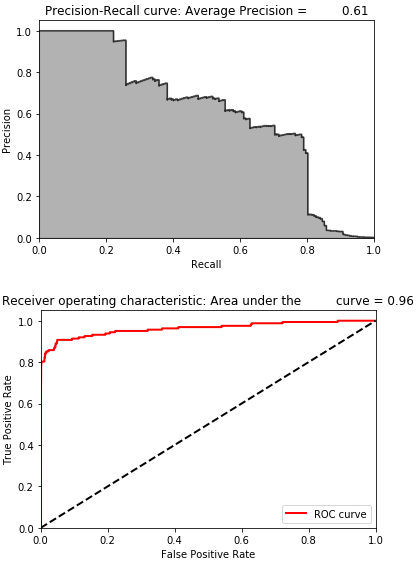
Figure 8-25 summarizes the distribution of average precisions across the 10 runs. The mean of the average precision is 0.24, worse than the 0.53 we achieved earlier. The coefficient of variation is 0.62.

Figure 8-25. Summary over 10 runs of sparse overcomplete autoencoder with single hidden layer, dropout, and linear activation function

Working with Noisy Datasets

A common problem with real-world data is the noisiness of the data - the data is distorted in some way because of data quality issues that may arise from data capture, data migration, data transformation, etc.

We need autoencoders to be robust enough against such noise so that they are not fooled by this type of noise and can learn from the truly important underlying structure in the data.

To simulate this noise, let’s add a Gaussian random matrix of noise to our credit card transactions dataset and then train an autoencoder on this noisy training set. Then, we will see how well the autoencoder does in predicting fraud on the noisy test set.

noise_factor = 0.50
X_train_AE_noisy = X_train_AE.copy() + noise_factor * \
 np.random.normal(loc=0.0, scale=1.0, size=X_train_AE.shape)
X_test_AE_noisy = X_test_AE.copy() + noise_factor * \
 np.random.normal(loc=0.0, scale=1.0, size=X_test_AE.shape)

Denoising Autoencoder

Compared to the original, non-distorted dataset, the penalty for overfitting to the noisy dataset of credit card transactions is much higher.

There is enough noise in the dataset that an autoencoder that fits too well to the noisy data will have a poor time detecting fraudulent transactions from normal ones.

This should make sense. We need an autoencoder that fits well enough to the data so that it is able to reconstruct most of the observations well enough but not so well enough that it accidentally reconstructs the noise, too.

In other words, we want the autoencoder to learn the underlying structure but forget the noise in the data.

Let’s try a few options from what has worked well so far. First, we will try a single hidden layer, 27-node undercomplete autoencoder with linear activation.

Next, we will try a single hidden layer, 40-node sparse overcomplete autoencoder with dropout.

And, finally, we will use an autoencoder with a non-linear activation function.

Two-Layer Denoising Undercomplete Autoencoder with Linear Activation

On the noisy dataset, the single hidden layer autoencoder with linear activation and 27 nodes had an average precision of 0.69. Let’s see how well it does on the noisy dataset. This autoencoder - because it is working with a noisy dataset and trying to denoise it - is known as a denoising autoencoder.

The code is similar to what we had before except now we are applying it to the noisy training and test datasets, X_train_AE_noisy and X_test_AE_noisy, respectively.

for i in range(0,10):
    # Call neural network API
    model = Sequential()

    # Generate hidden layer with 27 nodes using linear activation
    model.add(Dense(units=27, activation='linear', input_dim=29))

    # Generate output layer with 29 nodes
    model.add(Dense(units=29, activation='linear'))

    # Compile the model
    model.compile(optimizer='adam',
                  loss='mean_squared_error',
                  metrics=['accuracy'])

    # Train the model
    num_epochs = 10
    batch_size = 32

    history = model.fit(x=X_train_AE_noisy, y=X_train_AE_noisy,
                        epochs=num_epochs,
                        batch_size=batch_size,
                        shuffle=True,
                        validation_data=(X_train_AE, X_train_AE),
                        verbose=1)

    # Evaluate on test set
    predictions = model.predict(X_test_AE_noisy, verbose=1)
    anomalyScoresAE = anomalyScores(X_test, predictions)
    preds, avgPrecision = plotResults(y_test, anomalyScoresAE, True)
    test_scores.append(avgPrecision)
    model.reset_states()

print("Mean average precision over 10 runs: ", np.mean(test_scores))
test_scores

Figure 8-26 shows the losses from this autoencoder, and Figure 8-27 displays the average precision, the precision-recall curve, and the area under the ROC curve.

Figure 8-26. Training history of denoising undercomplete autoencoder with single hidden layer and linear activation function

Figure 8-27. Evaluation metrics of denoising undercomplete autoencoder with single hidden layer and linear activation function

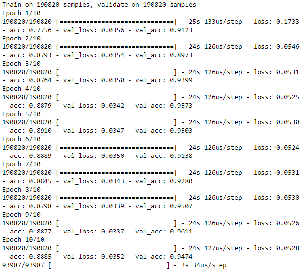
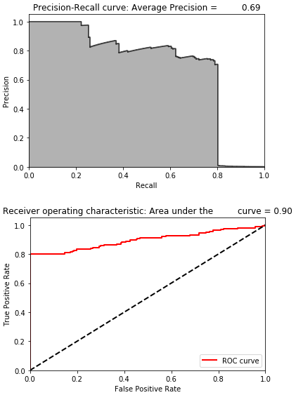
Figure 8-28 summarizes the distribution of average precisions across the 10 runs. The mean of the average precision is 0.24, worse than the 0.53 we achieved earlier. The coefficient of variation is 0.62.

Figure 8-28. Summary over 10 runs of denoising undercomplete autoencoder with single hidden layer and linear activation function

The mean average precision is now 0.28. You can see just how difficult it is for a linear autoencoder to denoise this noisy dataset. It struggles with separating the true underlying structure in the data from the Gaussian noise we added.

Two-Layer Denoising Overcomplete Autoencoder with Linear Activation

Let’s now try a single hidden layer overcomplete autoencoder with 40 nodes, a sparsity regularizer, and dropout of 0.05%.

This had an average precision of 0.56 on the original dataset.

model = Sequential()
model.add(Dense(units=40, activation='linear',
 activity_regularizer=regularizers.l1(10e-5),
                input_dim=29))
model.add(Dropout(0.05))
model.add(Dense(units=29, activation='linear'))

Figure 8-29 shows the losses from this autoencoder, and Figure 8-30 displays the average precision, the precision-recall curve, and the area under the ROC curve.

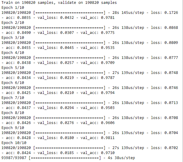
Figure 8-29. Training history of denoising overcomplete autoencoder with dropout and linear activation function

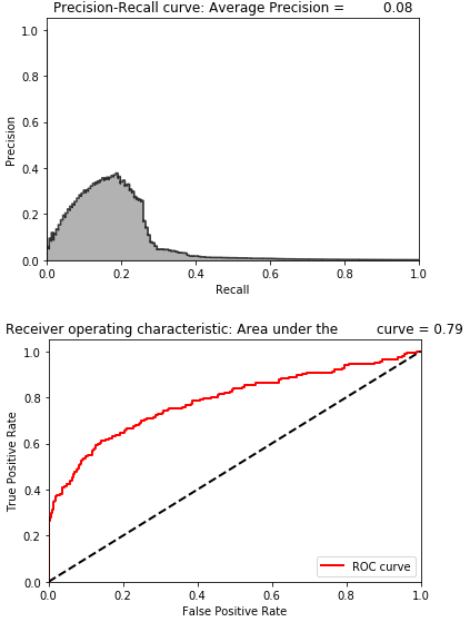
Figure 8-30. Evaluation metrics of denoising overcomplete autoencoder with dropout and linear activation function”

Figure 8-31 summarizes the distribution of average precisions across the 10 runs. The mean of the average precision is 0.10, worse than the 0.53 we achieved earlier. The coefficient of variation is 0.83.

Figure 8-31. Summary over 10 runs of denoising undercomplete autoencoder with single hidden layer and linear activation function

Two-Layer Denoising Overcomplete Autoencoder with ReLu Activation

Finally, let’s see how the same autoencoder fares using ReLu as the activation function instead of a linear activation function. Recall that the non-linear activation function autoencoder did not perform quite as well as the one with linear activation on the original dataset.

model = Sequential()
    model.add(Dense(units=40, activation='relu',  \
        activity_regularizer=regularizers.l1(10e-5), input_dim=29))
    model.add(Dropout(0.05))
model.add(Dense(units=29, activation='relu'))

Figure 8-32 shows the losses from this autoencoder, and Figure 8-33 displays the average precision, the precision-recall curve, and the area under the ROC curve.

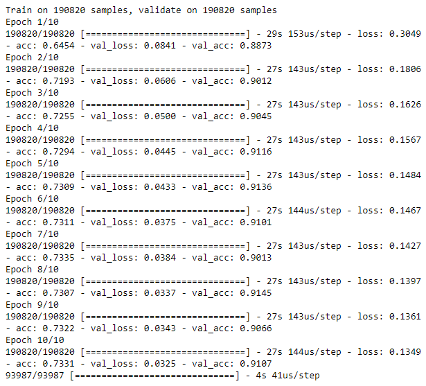
Figure 8-32. Training history of denoising overcomplete autoencoder with dropout and ReLU activation function”

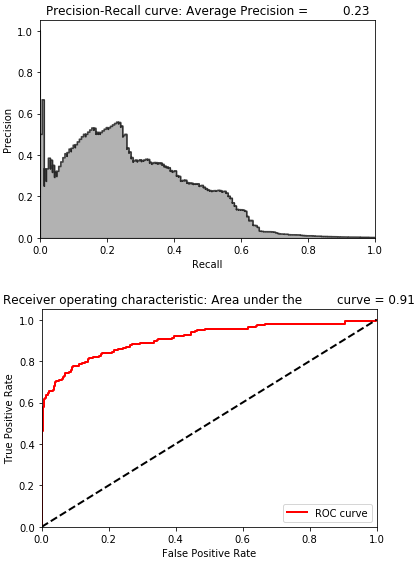
Figure 8-33. Evaluation metrics of denoising overcomplete autoencoder with dropout and ReLU activation function”

Figure 8-34 summarizes the distribution of average precisions across the 10 runs. The mean of the average precision is 0.20, worse than the 0.53 we achieved earlier. The coefficient of variation is 0.55.

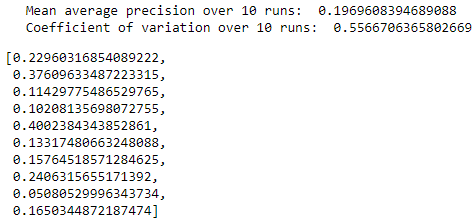
Figure 8-34. Summary over 10 runs of denoising overcomplete autoencoder with dropout and ReLU activation function”

You can experiment with the number of nodes, layers, degree of sparsity, dropout percentage, and the activation functions to see if you can improve the results from here.

Conclusion

In this chapter, we returned to the credit card fraud problem from earlier in the book to develop a neural network-based unsupervised fraud detection solution.

To find the optimal architecture for our autoencoder, we experimented with a variety of autoencoders. We tried complete, undercomplete, and overcomplete autoencoders with either a single or a few hidden layers. We also used both linear and non-linear activation functions and employed two major types of regularization, sparsity and dropout.

We found that a pretty simple two-layer undercomplete neural network with linear activation works best on the original credit card dataset, but we needed a sparse two-layer overcomplete autoencoder with linear activation and dropout to address the noise in the noisy credit card dataset.

A lot of our experiments were based on trial and error - for each experiment, we adjusted several hyperparameters and compared results with previous iterations. It is possible that an even better autoencoder-based fraud detection solution exists, and I encourage you to experiment on your own to find this.

So far in this book, we have viewed supervised and unsupervised as separate and distinct approaches, but, in the next chapter, we will explore how to employ both supervised and unsupervised approaches jointly to develop a so-called semi-supervised solution that is better than either standalone approach.