GANs, the Concept

GANs were introduced by Ian Goodfellow and his fellow researchers at the University of Montreal in 2014. In GANs, we have two neural networks. One network known as the generator generates data based on a model it has created using samples of real data it has received as input. The other network known as the discriminator discriminates between the data created by the generator and data from the true distribution.

As a simple analogy, the generator is the counterfeiter, and the discriminator is the police trying to identify the forgery. The two networks are locked in a zero-sum game. The generator is trying to fool the discriminator into thinking the synthetic data comes from the true distribution, and the discriminator is trying to call out the synthetic data as fake.

GANs are unsupervised learning algorithms because the generator can learn the underlying structure of the true distribution even when there are no labels. The generator learns the underlying structure by using a number of parameters significantly smaller than the amount of data it has trained on - a core concept of unsupervised learning that we have explored many times in previous chapters. This constraint forces the generator to efficiently capture the most salient aspects of the true data distribution.

This is similar to the representation learning that occurs in deep learning. Each hidden layer in the neutral network of a generator captures a representation of the underlying data—starting very simply—and subsequent layers pick up more complicated representations by building on the simpler preceding layers.

Using all these layers together, the generator learns the underlying structure of the data and attempts to create synthetic data that is nearly identical to the true data. If the generator has captured the essence of the true data, the synthetic data will appear real.

Deep Convolutional GANs (DCGANs)

In this chapter, we will return to the MNIST dataset we have used in previous chapters, and we will apply a version of GANs to generate synthetic data to supplement the existing MNIST dataset. We will then apply a supervised learning model to perform image classification. This is yet another version of semi-supervised learning.

The version of GANs we will use is called deep convolutional generative adversarial networks (DCGANs), which were first introduced in late 2015 by Alec Radford, Luke Metz, and Soumith Chintala.¹

DCGANs are an unsupervised learning form of convolution neural networks (CNNs), which are commonly used - and with great success - in supervised learning systems for computer vision and image classification. Before we delve into DCGANs, let’s explore CNNs first, especially how they are used for image classification in supervised learning systems.

Convolutional Neural Networks (CNNs)

Compared to numerical and text data, images and video are considerably more computationally expensive to work with. For instance, a 4K Ultra HD image has dimensions of 4096 x 2160 x 3 (26,542,080) in total. To train a neural network on images of this resolution directly would require tens of millions of neurons and result in very long training times.

Instead of building a neural network directly on the raw images, we can take advantage of certain properties of images, namely that pixels are related to other pixels that are close by but not usually related to other pixels that are far away.

Convolution - from which convolutional neural networks derive their name - is the process of filtering the image to decrease the size of the image without losing the relationships among pixels.²

On the original image, we apply several filters of a certain size, known as the kernel size, and move these filters with a small step, known as the stride, to derive the new reduced pixel output.

After the convolution, we reduce the size of the representation further by taking the max of the pixels in the reduced pixel output, one small area at a time. This is known as max pooling.

We perform this convolution and max pooling several times to reduce the complexity of the images. Then, we flatten the images and use a normal fully connected layer to perform image classification.

Let’s now build a CNN and use it to perform image classification on the MNIST dataset.

First, we will load the necessary libraries.

'''Main'''
import numpy as np
import pandas as pd
import os, time, re
import pickle, gzip, datetime

'''Data Viz'''
import matplotlib.pyplot as plt
import seaborn as sns
color = sns.color_palette()
import matplotlib as mpl
from mpl_toolkits.axes_grid1 import Grid

%matplotlib inline

'''Data Prep and Model Evaluation'''
from sklearn import preprocessing as pp
from sklearn.model_selection import train_test_split
from sklearn.model_selection import StratifiedKFold
from sklearn.metrics import log_loss, accuracy_score
from sklearn.metrics import precision_recall_curve, average_precision_score
from sklearn.metrics import roc_curve, auc, roc_auc_score, mean_squared_error

'''Algos'''
import lightgbm as lgb

'''TensorFlow and Keras'''
import tensorflow as tf
import keras
from keras import backend as K
from keras.models import Sequential, Model
from keras.layers import Activation, Dense, Dropout, Flatten, Conv2D, MaxPool2D
from keras.layers import LeakyReLU, Reshape, UpSampling2D, Conv2DTranspose
from keras.layers import BatchNormalization, Input, Lambda
from keras.layers import Embedding, Flatten, dot
from keras import regularizers
from keras.losses import mse, binary_crossentropy
from IPython.display import SVG
from keras.utils.vis_utils import model_to_dot
from keras.optimizers import Adam, RMSprop
from tensorflow.examples.tutorials.mnist import input_data

Next, we will load the MNIST datasets and store the image data in a 4D tensor since Keras requires image data in this format. We will also create one-hot vectors from the labels using the to_categorical function in Keras.

For use later, we will create Pandas DataFrames from the data, too. And, let’s re-use the view_digit function from earlier in the book to view the images.

# Load the datasets
current_path = os.getcwd()
file = '\\datasets\\mnist_data\\mnist.pkl.gz'
f = gzip.open(current_path+file, 'rb')
train_set, validation_set, test_set = pickle.load(f, encoding='latin1')
f.close()

X_train, y_train = train_set[0], train_set[1]
X_validation, y_validation = validation_set[0], validation_set[1]
X_test, y_test = test_set[0], test_set[1]

X_train_keras = X_train.reshape(50000,28,28,1)
X_validation_keras = X_validation.reshape(10000,28,28,1)
X_test_keras = X_test.reshape(10000,28,28,1)

y_train_keras = to_categorical(y_train)
y_validation_keras = to_categorical(y_validation)
y_test_keras = to_categorical(y_test)

# Create Pandas DataFrames from the datasets
train_index = range(0,len(X_train))
validation_index = range(len(X_train),len(X_train)+len(X_validation))
test_index = range(len(X_train)+len(X_validation),len(X_train)+ \
                   len(X_validation)+len(X_test))

X_train = pd.DataFrame(data=X_train,index=train_index)
y_train = pd.Series(data=y_train,index=train_index)

X_validation = pd.DataFrame(data=X_validation,index=validation_index)
y_validation = pd.Series(data=y_validation,index=validation_index)

X_test = pd.DataFrame(data=X_test,index=test_index)
y_test = pd.Series(data=y_test,index=test_index)

def view_digit(X, y, example):
    label = y.loc[example]
    image = X.loc[example,:].values.reshape([28,28])
    plt.title('Example: %d  Label: %d' % (example, label))
    plt.imshow(image, cmap=plt.get_cmap('gray'))
    plt.show()

Now let’s build the convolutional neural network.

We will call Sequential() in Keras to begin the model creation. Then, we will add two convolution layers, each with 32 filters of a kernel size of 5x5, a default stride of 1, and a rectified linear unit (ReLU) activation. Then, we perform max pooling with a pooling window of 2x2 and a stride of 1. And, we perform dropout, which you may recall is a form of regularization to reduce overfitting of the neural network. Specifically, we will drop 25% of the input units.

In the next stage, we add two convolution layers again, this time with 64 filters of a kernel size of 3x3. Then, we perform max pooling with a pooling window of 2x2 and a stride of 2. And, we follow this up with a dropout layer, with a dropout percentage of 25%.

Finally, we flatten the images, add a regular neural network with 256 hidden units, perform dropout with a dropout percentage of 50%, and perform 10-class classification using the softmax function.

model = Sequential()

model.add(Conv2D(filters = 32, kernel_size = (5,5), padding = 'Same',
                 activation ='relu', input_shape = (28,28,1)))
model.add(Conv2D(filters = 32, kernel_size = (5,5), padding = 'Same',
                 activation ='relu'))
model.add(MaxPooling2D(pool_size=(2,2)))
model.add(Dropout(0.25))


model.add(Conv2D(filters = 64, kernel_size = (3,3), padding = 'Same',
                 activation ='relu'))
model.add(Conv2D(filters = 64, kernel_size = (3,3), padding = 'Same',
                 activation ='relu'))
model.add(MaxPooling2D(pool_size=(2,2), strides=(2,2)))
model.add(Dropout(0.25))


model.add(Flatten())
model.add(Dense(256, activation = "relu"))
model.add(Dropout(0.5))
model.add(Dense(10, activation = "softmax"))

For this CNN training, we will use the Adam optimizer and minimize the cross entropy. We will also store the accuracy of the image classification as the evaluation metric.

Now, let’s train the model for one hundred epochs and evaluate the results on the validation set.

# Train CNN
model.compile(optimizer='adam',
              loss='categorical_crossentropy',
              metrics=['accuracy'])

model.fit(X_train_keras, y_train_keras,
          validation_data=(X_validation_keras, y_validation_keras), \
          epochs=100)

Figure 12-1 displays the final accuracy and the accuracy over the one hundred epochs of training.

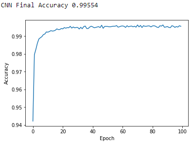
Figure 12-1. CNN results

As you can see, the CNN we just trained has a final accuracy of 99.55%, better than any of the MNIST image classification solutions we have trained so far throughout this book.

DCGANs Revisited

Let’s now turn back to deep convolutional generative adversarial networks once again. We will build a generative model to produce synthetic MNIST images that are very similar to the original MNIST images.

To produce near-realistic yet synthetic images, we need to train a generator that generates new images from the original MNIST images and a discriminator that judges whether those images are believably similar to the original ones or not (essentially performing a bullshit test).

Here is another way to think about this. The original MNIST dataset represents the original data distribution. The generator learns from this original distribution and generates new images based off what it has learned, and the discriminator attempts to determine whether the newly generated images are virtually indistinguishable from the original distribution or not.

For the generator, we will use the architecture presented in the Radford, Metz, and Chintala paper presented at the ICLR 2016 conference, which we referenced earlier (see Figure 12-2).

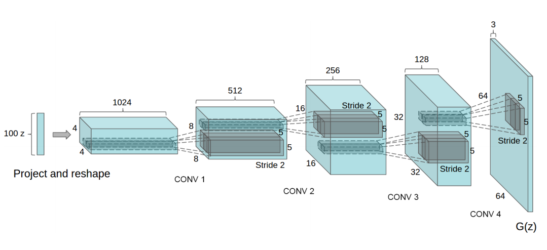
Figure 12-2. DCGAN generator

The genetor takes in an initial noise vector, shown as a 100x1 noise vector here denoted as z, and then projects and reshapes it into a 1024x4x4 tensor. This project and reshape action is the opposite of convolution and is known as tranposed convolution (or deconvolution in some cases). In transposed convolution, the original process of convolution is reversed, mapping a reduced tensor to a larger one.³

After the initial transposed convolution, the generator applies four additional deconvolution layers to map to a final 64x3x3 tensor.

Here are the various stages.

100x1 → 1024x4x4 → 512x8x8 → 256x16x16 → 128x32x32 → 64x64x3

We will apply a similar (but not exact) architecture when designing a DCGAN on the MNIST dataset.

def generator(self, depth=256, dim=7, dropout=0.3, momentum=0.8, \
              window=5, input_dim=100, output_depth=1):
    if self.G:
        return self.G
    self.G = Sequential()
    self.G.add(Dense(dim*dim*depth, input_dim=input_dim))
    self.G.add(BatchNormalization(momentum=momentum))
    self.G.add(Activation('relu'))
    self.G.add(Reshape((dim, dim, depth)))
    self.G.add(Dropout(dropout))

    self.G.add(UpSampling2D())
    self.G.add(Conv2DTranspose(int(depth/2), window, padding='same'))
    self.G.add(BatchNormalization(momentum=momentum))
    self.G.add(Activation('relu'))

    self.G.add(UpSampling2D())
    self.G.add(Conv2DTranspose(int(depth/4), window, padding='same'))
    self.G.add(BatchNormalization(momentum=momentum))
    self.G.add(Activation('relu'))

    self.G.add(Conv2DTranspose(int(depth/8), window, padding='same'))
    self.G.add(BatchNormalization(momentum=momentum))
    self.G.add(Activation('relu'))

    self.G.add(Conv2DTranspose(output_depth, window, padding='same'))
    self.G.add(Activation('sigmoid'))
    self.G.summary()
    return self.G

def discriminator(self, depth=64, dropout=0.3, alpha=0.3):
    if self.D:
        return self.D
    self.D = Sequential()
    input_shape = (self.img_rows, self.img_cols, self.channel)
    self.D.add(Conv2D(depth*1, 5, strides=2, input_shape=input_shape,
        padding='same'))
    self.D.add(LeakyReLU(alpha=alpha))
    self.D.add(Dropout(dropout))

    self.D.add(Conv2D(depth*2, 5, strides=2, padding='same'))
    self.D.add(LeakyReLU(alpha=alpha))
    self.D.add(Dropout(dropout))

    self.D.add(Conv2D(depth*4, 5, strides=2, padding='same'))
    self.D.add(LeakyReLU(alpha=alpha))
    self.D.add(Dropout(dropout))

    self.D.add(Conv2D(depth*8, 5, strides=1, padding='same'))
    self.D.add(LeakyReLU(alpha=alpha))
    self.D.add(Dropout(dropout))

    self.D.add(Flatten())
    self.D.add(Dense(1))
    self.D.add(Activation('sigmoid'))
    self.D.summary()
    return self.D

def discriminator_model(self):
    if self.DM:
        return self.DM
    optimizer = RMSprop(lr=0.0002, decay=6e-8)
    self.DM = Sequential()
    self.DM.add(self.discriminator())
    self.DM.compile(loss='binary_crossentropy', \
                    optimizer=optimizer, metrics=['accuracy'])
    return self.DM

def adversarial_model(self):
    if self.AM:
        return self.AM
    optimizer = RMSprop(lr=0.0001, decay=3e-8)
    self.AM = Sequential()
    self.AM.add(self.generator())
    self.AM.add(self.discriminator())
    self.AM.compile(loss='binary_crossentropy', \
                    optimizer=optimizer, metrics=['accuracy'])
    return self.AM

class MNIST_DCGAN(object):
    def __init__(self, x_train):
        self.img_rows = 28
        self.img_cols = 28
        self.channel = 1

        self.x_train = x_train

        self.DCGAN = DCGAN()
        self.discriminator =  self.DCGAN.discriminator_model()
        self.adversarial = self.DCGAN.adversarial_model()
        self.generator = self.DCGAN.generator()

def train(self, train_steps=2000, batch_size=256, save_interval=0):
    noise_input = None
    if save_interval>0:
        noise_input = np.random.uniform(-1.0, 1.0, size=[16, 100])
    for i in range(train_steps):
        images_train = self.x_train[np.random.randint(0,
            self.x_train.shape[0], size=batch_size), :, :, :]
        noise = np.random.uniform(-1.0, 1.0, size=[batch_size, 100])
        images_fake = self.generator.predict(noise)
        x = np.concatenate((images_train, images_fake))
        y = np.ones([2*batch_size, 1])
        y[batch_size:, :] = 0

        d_loss = self.discriminator.train_on_batch(x, y)

        y = np.ones([batch_size, 1])
        noise = np.random.uniform(-1.0, 1.0, size=[batch_size, 100])
        a_loss = self.adversarial.train_on_batch(noise, y)
        log_mesg = "%d: [D loss: %f, acc: %f]" % (i, d_loss[0], d_loss[1])
        log_mesg = "%s  [A loss: %f, acc: %f]" % (log_mesg, a_loss[0], \
                                                  a_loss[1])
        print(log_mesg)
        if save_interval>0:
            if (i+1)%save_interval==0:
                self.plot_images(save2file=True, \
                    samples=noise_input.shape[0],\
                    noise=noise_input, step=(i+1))

def plot_images(self, save2file=False, fake=True, samples=16, \
                noise=None, step=0):
    filename = 'mnist.png'
    if fake:
        if noise is None:
            noise = np.random.uniform(-1.0, 1.0, size=[samples, 100])
        else:
            filename = "mnist_%d.png" % step
        images = self.generator.predict(noise)
    else:
        i = np.random.randint(0, self.x_train.shape[0], samples)
        images = self.x_train[i, :, :, :]

    plt.figure(figsize=(10,10))
    for i in range(images.shape[0]):
        plt.subplot(4, 4, i+1)
        image = images[i, :, :, :]
        image = np.reshape(image, [self.img_rows, self.img_cols])
        plt.imshow(image, cmap='gray')
        plt.axis('off')
    plt.tight_layout()
    if save2file:
        plt.savefig(filename)
        plt.close('all')
    else:
        plt.show()

MNIST DCGAN in Action

Now that we have defined the MNIST_DCGAN call, let’s call it and begin the training process. We will train for 10,000 epochs with a batch size of 256.

# Initialize MNIST_DCGAN and train
mnist_dcgan = MNIST_DCGAN(X_train_keras)
timer = ElapsedTimer()
mnist_dcgan.train(train_steps=10000, batch_size=256, save_interval=500)

Figure 12-3 displays the loss and the accuracy of the discriminator and the adversarial model.

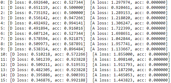
Figure 12-3. Initial loss of the MNIST DCGAN

The initial loss of the discriminator fluctuates wildly but remains considerably above 0.50. In other words, the discriminator is initially very good at catching the poorly constructured counterfeits from the generator. Then, as the generator becomes better at creating counterfeits, the discriminator struggles; its accuracy drops close to 0.50 (see Figure 12-4).

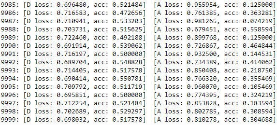
Figure 12-4. Final loss of the MNIST DCGAN

Synthetic Image Generation

Now that the MNIST DCGAN has been trained, let’s use it to generate a sample of synthetic images (see Figure 12-5).

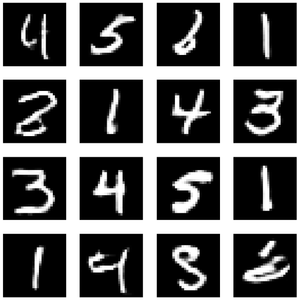
Figure 12-5. Synthetic images generated by the MNIST DCGAN

These synthetic images - while not entirely indistinguishable from the real MNIST dataset - are eeriely similar to real digits. With more training time, the MNIST DCGAN should be capable of generating synthetic images that more closely resemble those of the real MNIST dataset and could be used to supplement the size of that dataset.

While our solution is reasonably good, there are many ways to make the MNIST DCGAN perform better. Here is a paper and the accomanying code that delves into more advanced methods to improve GAN performance.

Conclusion

In this chapter, we explored deep convolutional generative adversarial networks, a specialized form of generative adversarial networks that perform well on image and computer vision datasets.

GANs are a generative model with two neural networks locked in a zero-sum game. One of the networks, the generator (i.e., the counterfeiter), is generating synthetic data from real data, while the other network, the discriminator (i.e, the police), is calling the counterfeits as fake or real.⁶

This zero-sum game in which the generator learns from the discriminator leads to an overall generative model that generates pretty realistic synthetic data and generally gets better over time (i.e., as we train for more training epochs).

GANs are relatively new - they were first introduced by Ian Goodfellow et al. in 2014.⁷. GANs are currently mainly used to perform anomaly detection and generate synthetic data, but they could have many other applications in the near future. The machine learning community is barely scratching the surface with what is possible, and, if you decide to use GANs in applied machine learning systems, be ready to experiment a lot.⁸

In Chapter 13, we will explore our last and final concept called temporal clustering, which are a form of unsupervised learning for use with time series data.