The Motivation for Dimensionality Reduction

As mentioned in Chapter 1, dimensionality reduction helps counteract one of the most commonly occurring problems in machine learning - the curse of dimensionality - in which algorithms cannot effectively and efficiently train on the data because of the sheer size of the feature space.

Dimensionality reduction algorithms project high-dimensional data to a low-dimensional space, retaining as much of the salient information as possible while removing redundant information. Once the data is in the low-dimensional space, machine learning algorithms are able to identify interesting patterns more effectively and efficiently because a lot of the noise has been reduced.

Sometimes, dimensionality reduction is the goal itself - for example, to build anomaly detection systems as we will show in the next chapter.

Other times, dimensionality reduction is not an end in itself but rather a means to another end. For example, dimensionality reduction is commonly a part of the machine learning pipeline to help solve large-scale, computationally expensive problems involving images, video, speech, and text.

The MNIST Digits Database

Before we introduce the dimensionality reduction algorithms, let’s explore the dataset that we will use in this chapter. We will work with a simple computer vision dataset - the MNIST (Mixed National Institute of Standards and Technology) database of handwritten digits - one of the best known datasets in machine learning. We will use the version of the MNIST dataset publicly available on Yann LeCun’s website.¹ To make it easier, we will use the pickled version of this, courtesy of deeplearning.net.²

This dataset has been divided into three sets already - a training set with 50,000 examples, a validation set with 10,000 examples, and a test set with 10,000 examples. We have labels for all the examples.

This dataset consists of 28x28 pixel images of handwritten digits. Every single data point (i.e., every image) can be conveyed as an array of numbers, where each number describes how dark each pixel is. In other words, a 28x28 array of numbers corresponds to a 28x28 pixel image.

To make this simpler, we can flatten each array into a 28x28, or 784, dimensional vector. Each component of the vector is a float between zero and one - representing the intensity of each pixel in the image. Zero stands for black, and one for white. The labels are numbers between zero and nine, indicating which digit the image represents.

Data acquisition and exploration

Before we work with the dimensionality reduction algorithms, let’s load the libraries we will use.

# Import libraries
'''Main'''
import numpy as np
import pandas as pd
import os, time
import pickle, gzip

'''Data Viz'''
import matplotlib.pyplot as plt
import seaborn as sns
color = sns.color_palette()
import matplotlib as mpl

%matplotlib inline

'''Data Prep and Model Evaluation'''
from sklearn import preprocessing as pp
from scipy.stats import pearsonr
from numpy.testing import assert_array_almost_equal
from sklearn.model_selection import train_test_split
from sklearn.model_selection import StratifiedKFold
from sklearn.metrics import log_loss
from sklearn.metrics import precision_recall_curve, average_precision_score
from sklearn.metrics import roc_curve, auc, roc_auc_score
from sklearn.metrics import confusion_matrix, classification_report

'''Algos'''
from sklearn.linear_model import LogisticRegression
from sklearn.ensemble import RandomForestClassifier
import xgboost as xgb
import lightgbm as lgb

Load the MNIST datasets

Let’s now load the MNIST datasets.

# Load the datasets
current_path = os.getcwd()
file = '\\datasets\\mnist_data\\mnist.pkl.gz'

f = gzip.open(current_path+file, 'rb')
train_set, validation_set, test_set = pickle.load(f, encoding='latin1')
f.close()

X_train, y_train = train_set[0], train_set[1]
X_validation, y_validation = validation_set[0], validation_set[1]
X_test, y_test = test_set[0], test_set[1]

Verify shape of datasets

Let’s verify the shape of the datasets to make sure they loaded properly.

# Verify shape of datasets
print("Shape of X_train: ", X_train.shape)
print("Shape of y_train: ", y_train.shape)
print("Shape of X_validation: ", X_validation.shape)
print("Shape of y_validation: ", y_validation.shape)
print("Shape of X_test: ", X_test.shape)
print("Shape of y_test: ", y_test.shape)

Figure 3-1 confirms the shapes of the datasets are as expected.

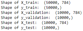
Figure 3-1. Shape of MNIST dataset

Create Pandas DataFrames from the datasets

Let’s convert the numpy arrays into Pandas DataFrames so they are easier to explore and work with.

# Create Pandas DataFrames from the datasets
train_index = range(0,len(X_train))
validation_index = range(len(X_train), /
                         len(X_train)+len(X_validation))
test_index = range(len(X_train)+len(X_validation), /
                   len(X_train)+len(X_validation)+len(X_test))

X_train = pd.DataFrame(data=X_train,index=train_index)
y_train = pd.Series(data=y_train,index=train_index)

X_validation = pd.DataFrame(data=X_validation,index=validation_index)
y_validation = pd.Series(data=y_validation,index=validation_index)

X_test = pd.DataFrame(data=X_test,index=test_index)
y_test = pd.Series(data=y_test,index=test_index)

Explore the data

Let’s generate a summary view of the data.

# Describe the training matrix
X_train.describe()

Figure 3-2 displays a summary view of the image data. Many of the values are zeros - in other words, most of the pixels in the images are black. This makes sense since the digits are in white and shown in the middle of the image on a black backdrop.

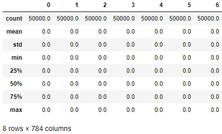
Figure 3-2. Data exploration

The labels data is a one-dimensional vector representing the actual number of the image. Figure 3-3 shows the labels for the first few images.

# Show the labels
y_train.head()

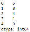
Figure 3-3. Labels preview

Display the images

Let’s define a function to view the image along with its label.

def view_digit(example):
    label = y_train.loc[0]
    image = X_train.loc[example,:].values.reshape([28,28])
    plt.title('Example: %d  Label: %d' % (example, label))
    plt.imshow(image, cmap=plt.get_cmap('gray'))
    plt.show()

A view of the first image - once the 784-dimensional vector is reshaped into a 28x28 pixel image - shows the number five (see Figure 3-4).

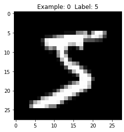
Figure 3-4. View the first digit

Dimensionality Reduction Algorithms

Now that we’ve loaded and explored the MNIST digits dataset, let’s move to the dimensionality reduction algorithms. For each algorithm, we will first introduce the concept and then build deeper intuition by applying the algorithm to the MNIST digits dataset.

Principal Component Analysis (PCA)

We will explore several versions of PCA, including standard PCA, incremental PCA, sparse PCA, and kernel PCA.³

PCA in Practice

Now that you have a better grasp of how PCA works, let’s apply PCA to the MNIST digits dataset and see how well PCA captures the most salient information about the digits as its projects the data from the original 784-dimensional space to a lower dimensional space.

Set the hyperparameters

Let’s set the hyperparameters for the PCA algorithm.

from sklearn.decomposition import PCA

n_components = 784
whiten = False
random_state = 2018

pca = PCA(n_components=n_components, whiten=whiten, \
          random_state=random_state)

Apply PCA

We will set the number of principal components to the original number of dimensions (i.e., 784). PCA will capture the salient information from the original dimensions and start generating principal components. Once these components are generated, we will determine how many principal components we need to effectively capture most of the variance/information from the original feature set.

Let’s fit and transform our training data, generating these principal components.

X_train_PCA = pca.fit_transform(X_train)
X_train_PCA = pd.DataFrame(data=X_train_PCA, index=train_index)

Evaluate PCA

Because we have not reduced the dimensionality at all - we’ve just transformed the data - the variance/information of the original data captured by the 784 principal components should be 100%.

Figure 3-5 confirms this.

# Percentage of Variance Captured by 784 principal components
print("Variance Explained by all 784 principal components: ", \
      sum(pca.explained_variance_ratio_))

Figure 3-5. Variance captured by all 784 principal components

However, it is important to note that the importance of the 784 principal components varies quite a bit. Figure 3-6 displays a summary of how important the first X principal components are.

# Percentage of Variance Captured by X principal components
importanceOfPrincipalComponents = \
    pd.DataFrame(data=pca.explained_variance_ratio_)
importanceOfPrincipalComponents = importanceOfPrincipalComponents.T

print('Variance Captured by First 10 Principal Components: ',
      importanceOfPrincipalComponents.loc[:,0:9].sum(axis=1).values)
print('Variance Captured by First 20 Principal Components: ',
      importanceOfPrincipalComponents.loc[:,0:19].sum(axis=1).values)
print('Variance Captured by First 50 Principal Components: ',
      importanceOfPrincipalComponents.loc[:,0:49].sum(axis=1).values)
print('Variance Captured by First 100 Principal Components: ',
      importanceOfPrincipalComponents.loc[:,0:99].sum(axis=1).values)
print('Variance Captured by First 200 Principal Components: ',
      importanceOfPrincipalComponents.loc[:,0:199].sum(axis=1).values)
print('Variance Captured by First 300 Principal Components: ',
      importanceOfPrincipalComponents.loc[:,0:299].sum(axis=1).values)

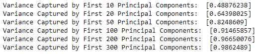
Figure 3-6. Variance captured by X principal components

The first 10 components in total capture approximately 50% of the variance, the first 100 components over 90%, and the first 300 components almost 99% of the variance; the information in the rest of the principal components is of negligible value.

We can also plot the importance of each principal component, ranked from the first principal component to the last. For the sake of readability, just the first 10 components are displayed in Figure 3-7.

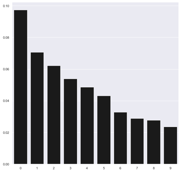
Figure 3-7. Importance of PCA components

The power of PCA should be more apparent now. With just the first 200 principal components - far fewer than the original 784 dimensions - we capture over 96% of the variance/information.

PCA allows us to reduce the dimensionality of the original data substantially while retaining most of the salient information. On the PCA-reduced feature set, other machine learning algorithms - downstream in the machine learning pipeline - will have an easier time separating the data points in space (to perform tasks such as anomaly detection and clustering) and will require fewer computational resources.

Visualize the separation of points in space

To demonstrate the power of PCA to efficiently and compactly capture the variance/information in data, let’s plot the observations in two dimensions. Specifically, we will display a scatter plot of the first and second principal components and mark the observations by the true label. Let’s create a function for this called scatterPlot because we need to present visualizations for the other dimensionality algorithms, too, later on.

def scatterPlot(xDF, yDF, algoName):
    tempDF = pd.DataFrame(data=xDF.loc[:,0:1], index=xDF.index)
    tempDF = pd.concat((tempDF,yDF), axis=1, join="inner")
    tempDF.columns = ["First Vector", "Second Vector", "Label"]
    sns.lmplot(x="First Vector", y="Second Vector", hue="Label", \
               data=tempDF, fit_reg=False)
    ax = plt.gca()
    ax.set_title("Separation of Observations using "+algoName)

scatterPlot(X_train_PCA, y_train, "PCA")

As seen in Figure 3-8, with just the top two principal components, PCA does a good job of separating the points in space such that similar points are generally closer to each other than they are to other, more different points. In other words, images of the same digit are closer to each other than they are to images of other digits.

PCA accomplishes this without using any labels whatsoever. This demonstrates the power of unsupervised learning to capture the underlying structure of data, helping discover hidden patterns in the absence of labels.

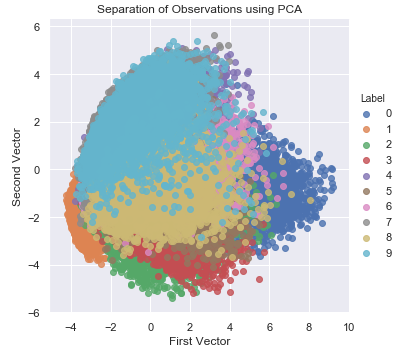
Figure 3-8. Separation of Observations Using PCA

If we run the same two-dimensional scatter plot using two of the most important features from the original 784 feature set - determined by training a supervised learning model - the separation is poor, at best (see Figure 3-9).

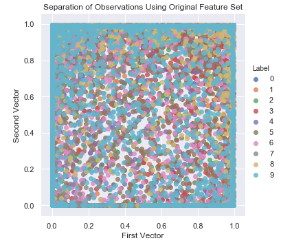
Figure 3-9. Separation of observations without PCA

The comparison of Figures 3-8 and 3-9 shows just how powerful PCA is in learning the underlying structure of the dataset without using any labels whatsoever - even with just two dimensions, we can start meaningfully separating the images by the digit they display.

Note

Not only does PCA help separate data so that we can discover hidden patterns more readily, PCA also helps reduce the size of the feature set, making it less costly - both in time and in computational resources - to train machine learning models.

With the MNIST dataset, the reduction in training time will be modest at best since the dataset is very small to begin with - we have only 784 features and 50,000 observations. But, if the dataset were millions of features and billions of observations, dimensionality reduction would dramatically reduce the training time of machine learning algorithms further along in the machine learning pipeline.

Lastly, PCA usually throws away some of the information available in the original feature set but does so wisely, capturing the most important elements and tossing the less valuable ones. A model that is trained on a PCA-reduced feature set may not perform quite as well in terms of accuracy as a model that is trained on the full feature set, but both the training and prediction times will be much faster. This is one of the important trade-offs you must consider when choosing whether to use dimensionality reduction in your machine learning product.

Incremental PCA

For datasets that are very, very large and cannot fit in memory, we can perform principal component analysis incrementally in small batches, where each batch is able to fit in memory. The batch size can be either set manually or determined automatically. This batch-based form of PCA is known as incremental PCA. The resulting principal components of PCA and incremental PCA are generally pretty similar (see Figure 3-10). Here is the code for incremental PCA.⁴

# Incremental PCA
from sklearn.decomposition import IncrementalPCA

n_components = 784
batch_size = None

incrementalPCA = IncrementalPCA(n_components=n_components, \
                                batch_size=batch_size)

X_train_incrementalPCA = incrementalPCA.fit_transform(X_train)
X_train_incrementalPCA = \
    pd.DataFrame(data=X_train_incrementalPCA, index=train_index)

X_validation_incrementalPCA = incrementalPCA.transform(X_validation)
X_validation_incrementalPCA = \
    pd.DataFrame(data=X_validation_incrementalPCA, index=validation_index)

scatterPlot(X_train_incrementalPCA, y_train, "Incremental PCA")

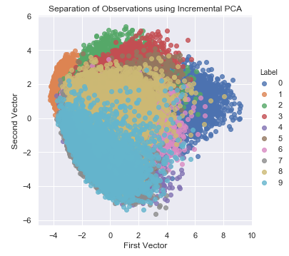
Figure 3-10. Separation of observations using incremental PCA

Sparse PCA

The normal PCA algorithm searches for linear combinations in all the input variables, reducing the original feature space as densely as possible. But, for some machine learning problems, some degree of sparsity may be preferred. A version of PCA that retains some degree of sparsity - controlled by a hyperparameter called alpha - is known as sparse PCA. The sparse PCA algorithm searches for linear combinations in just some of the input variables, reducing the original feature space to some degree but not as compactly as normal PCA.⁵

Because this algorithm trains a bit more slowly than normal PCA, we will train on just the first 10,000 examples in our training set (out of the total 50,000 examples). We will continue this practice of training on fewer than the total number of observations when the algorithm training times are slow.

For our purposes - developing some intuition of how these dimensionality reduction algorithms work - this reduced training process is fine. If you want a better solution, training on the complete training set is advised.

# Sparse PCA
from sklearn.decomposition import SparsePCA

n_components = 100
alpha = 0.0001
random_state = 2018
n_jobs = -1

sparsePCA = SparsePCA(n_components=n_components, \
                alpha=alpha, random_state=random_state, n_jobs=n_jobs)

sparsePCA.fit(X_train.loc[:10000,:])
X_train_sparsePCA = sparsePCA.transform(X_train)
X_train_sparsePCA = pd.DataFrame(data=X_train_sparsePCA, index=train_index)

X_validation_sparsePCA = sparsePCA.transform(X_validation)
X_validation_sparsePCA = \
    pd.DataFrame(data=X_validation_sparsePCA, index=validation_index)

scatterPlot(X_train_sparsePCA, y_train, "Sparse PCA")

Figure 3-11 shows a two-dimensional scatter plot using the first two principal components using sparse PCA.

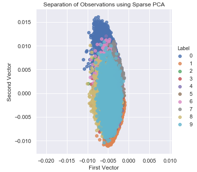
Figure 3-11. Separation of observations using sparse PCA

Notice that this scatterplot looks different from that of the normal PCA, as expected. Normal and sparse PCA generate principal components differently, and the separation of points is somewhat different, too.

Kernel PCA

Normal PCA, incremental PCA, and sparse PCA linearly project the original data onto a lower dimensional space, but there is also a non-linear form of PCA known as kernel PCA, which runs a similarity function over pairs of original data points in order to perform non-linear dimensionality reduction.⁶

By learning this similarity function - known as the kernel method - kernel PCA maps the implicit feature space where the majority of data points lie and creates this implicit feature space in a much smaller number of dimensions than the dimensions in the original feature set. This method is especially effective when the original feature set is not linearly separable.

For the kernel PCA algorithm, we need to set the number of components we desire, the type of kernel, and the kernel coefficient known as gamma. The most popular kernel is the radial basis function kernel, which is more commonly referred to as RBF kernel. This is what we will use.

# Kernel PCA
from sklearn.decomposition import KernelPCA

n_components = 100
kernel = 'rbf'
gamma = None
random_state = 2018
n_jobs = 1

kernelPCA = KernelPCA(n_components=n_components, kernel=kernel, \
                      gamma=gamma, n_jobs=n_jobs, random_state=random_state)

kernelPCA.fit(X_train.loc[:10000,:])
X_train_kernelPCA = kernelPCA.transform(X_train)
X_train_kernelPCA = pd.DataFrame(data=X_train_kernelPCA,index=train_index)

X_validation_kernelPCA = kernelPCA.transform(X_validation)
X_validation_kernelPCA = \
    pd.DataFrame(data=X_validation_kernelPCA, index=validation_index)

scatterPlot(X_train_kernelPCA, y_train, "Kernel PCA")

The two-dimensional scatter plot of kernel PCA is nearly identical to the one of the linear PCA for our MNIST digits dataset (see Figure 3-12). Learning the RBF kernel does not improve the dimensionality reduction.

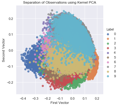
Figure 3-12. Separation of observations using kernel PCA

Singular Value Decomposition

Another approach to learn the underlying structure of the data is to reduce the rank of the original matrix of features to a smaller rank such that the original matrix can be re-created using a linear combination of some of the vectors in the smaller rank matrix. This is known as singular value decomposition (SVD).⁷

To generate the smaller rank matrix, SVD keeps the vectors of the original matrix that have the most information (i.e., the highest singular value). The smaller rank matrix captures the most important elements of the original feature space.

This should sound very similar to principal component analysis. PCA uses the eigen-decomposition of the covariance matrix to perform dimensionality reduction, while SVD uses singular value decomposition, as its name implies. In fact, PCA involves the use of SVD in its calculation, but much of this discussion is beyond the scope of this applied book.

# Singular Value Decomposition
from sklearn.decomposition import TruncatedSVD

n_components = 200
algorithm = 'randomized'
n_iter = 5
random_state = 2018

svd = TruncatedSVD(n_components=n_components, algorithm=algorithm, \
                   n_iter=n_iter, random_state=random_state)

X_train_svd = svd.fit_transform(X_train)
X_train_svd = pd.DataFrame(data=X_train_svd, index=train_index)

X_validation_svd = svd.transform(X_validation)
X_validation_svd = pd.DataFrame(data=X_validation_svd, index=validation_index)

scatterPlot(X_train_svd, y_train, "Singular Value Decomposition")

Figure 3-13 displays the separation of points that we achieve using the two most important vectors from SVD.

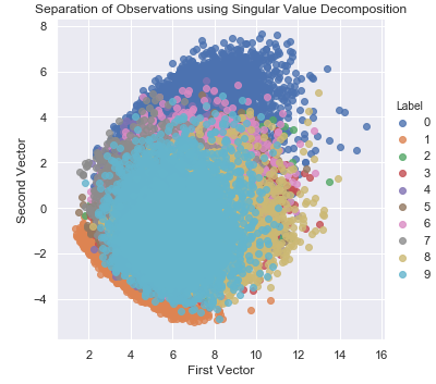
Figure 3-13. Separation of observations using SVD

Random Projection

Another linear dimensionality reduction technique is random projection, which relies on the Johnson-Lindenstrauss lemma. According to the Johnson-Lindenstrauss lemma, points in a high-dimensional space can be embedded into a much lower-dimensional space in such a way that distances between the points are nearly preserved. In other words, even as we move from high-dimensional space to low-dimensional space, the relevant structure of the original feature set is preserved.

Gaussian Random Projection

There are two versions of random projection - the standard version known as Gaussian random projection and a sparse version known as sparse random projection.

For Gaussian random projection, we can either specify the number of components we would like to have in the reduced feature space, or we can set the hyperparameter eps. This hyperparameter eps controls the quality of the embedding according to the Johnson-Lindenstrauss lemma, where smaller values generate a higher number of dimensions. In our case, we will set this hyperparameter.⁸

# Gaussian Random Projection
from sklearn.random_projection import GaussianRandomProjection

n_components = 'auto'
eps = 0.5
random_state = 2018

GRP = GaussianRandomProjection(n_components=n_components, eps=eps, \
                               random_state=random_state)

X_train_GRP = GRP.fit_transform(X_train)
X_train_GRP = pd.DataFrame(data=X_train_GRP, index=train_index)

X_validation_GRP = GRP.transform(X_validation)
X_validation_GRP = pd.DataFrame(data=X_validation_GRP, index=validation_index)

scatterPlot(X_train_GRP, y_train, "Gaussian Random Projection")

Figure 3-14 shows the two-dimensional scatter plot using Gaussian random projection.

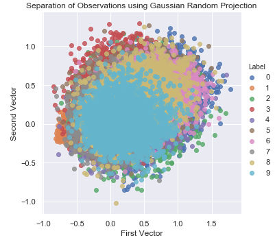
Figure 3-14. Separation of observations using gaussian random projection

Although it is a form of linear projection like PCA, random projection is an entirely different family of dimensionality reduction. Therefore the random projection scatterplot looks very different from the scatterplots from normal PCA, incremental PCA, sparse PCA, and kernel PCA.

Sparse Random Projection

Just as there is a sparse version of PCA, there is a sparse version of random projection known as sparse random projection, which retains some degree of sparsity in the transformed feature set. Sparse random projection is generally much more efficient, transforming the original data into the reduced space much faster than normal Gaussian random projection.⁹

# Sparse Random Projection
from sklearn.random_projection import SparseRandomProjection

n_components = 'auto'
density = 'auto'
eps = 0.5
dense_output = False
random_state = 2018

SRP = SparseRandomProjection(n_components=n_components, \
        density=density, eps=eps, dense_output=dense_output, \
        random_state=random_state)

X_train_SRP = SRP.fit_transform(X_train)
X_train_SRP = pd.DataFrame(data=X_train_SRP, index=train_index)

X_validation_SRP = SRP.transform(X_validation)
X_validation_SRP = pd.DataFrame(data=X_validation_SRP, index=validation_index)

scatterPlot(X_train_SRP, y_train, "Sparse Random Projection")

Figure 3-15 shows the two-dimensional scatter plot using sparse random projection.

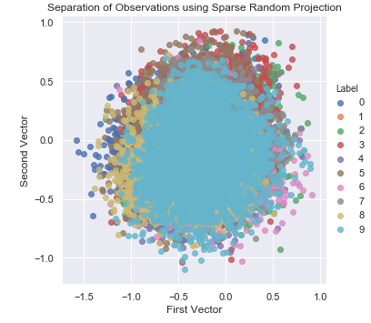
Figure 3-15. Separation of observations using sparse random projection

Isomap

Instead of linearly projecting the data from a high dimensional space to a low dimensional space, we can use non-linear dimensionality reduction methods. These methods are collectively known as manifold learning.

The most vanilla form of manifold learning is known as isometric mapping, or Isomap for short. Like kernel PCA, Isomap learns a new, low-dimensional embedding of the original feature set by calculating the pairwise distances of all the points, where distance is the curved or geodesic distance rather than Euclidean distance. In other words, it learns the intrinsic geometry of the original data based on where each point lies relative to its neighbors on a manifold.

# Isomap

from sklearn.manifold import Isomap

n_neighbors = 5
n_components = 10
n_jobs = 4

isomap = Isomap(n_neighbors=n_neighbors, \
                n_components=n_components, n_jobs=n_jobs)

isomap.fit(X_train.loc[0:5000,:])
X_train_isomap = isomap.transform(X_train)
X_train_isomap = pd.DataFrame(data=X_train_isomap, index=train_index)

X_validation_isomap = isomap.transform(X_validation)
X_validation_isomap = pd.DataFrame(data=X_validation_isomap, \
                                   index=validation_index)

scatterPlot(X_train_isomap, y_train, "Isomap")

Figure 3-16 shows the two-dimensional scatter plot using Isomap.

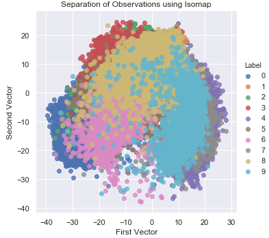
Figure 3-16. Separation of observations using isomap

Multidimensional Scaling (MDS)

Multidimensional scaling (MDS) is a form of non-linear dimensionality reduction that learns the similarity of points in the original dataset and, using this similarity learning, models this in a lower dimensional space.¹⁰

# Multidimensional Scaling
from sklearn.manifold import MDS

n_components = 2
n_init = 12
max_iter = 1200
metric = True
n_jobs = 4
random_state = 2018

mds = MDS(n_components=n_components, n_init=n_init, max_iter=max_iter, \
          metric=metric, n_jobs=n_jobs, random_state=random_state)

X_train_mds = mds.fit_transform(X_train.loc[0:1000,:])
X_train_mds = pd.DataFrame(data=X_train_mds, index=train_index[0:1001])

scatterPlot(X_train_mds, y_train, "Multidimensional Scaling")

Figure 3-17 displays the two-dimensional scatter plot using multidimensional scaling (MDS).

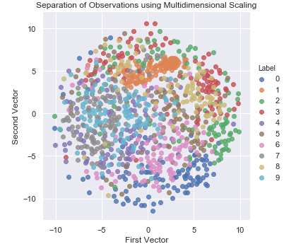
Figure 3-17. Separation of observations using MDS

Locally Linear Embedding

Another popular non-linear dimensionality reduction method is locally linear embedding (LLE), which preserves distances within local neighborhoods as it projects the data from the original feature space to a reduced space. LLE discovers the non-linear structure in the original, high dimensional data by segmenting the data into smaller components (i.e., into neighborhoods of points) and modeling each component as a linear embedding.¹¹

For this algorithm, we set the number of components we desire and the number of points to consider in a given neighborhood.

# Locally Linear Embedding (LLE)
from sklearn.manifold import LocallyLinearEmbedding

n_neighbors = 10
n_components = 2
method = 'modified'
n_jobs = 4
random_state = 2018

lle = LocallyLinearEmbedding(n_neighbors=n_neighbors, \
        n_components=n_components, method=method, \
        random_state=random_state, n_jobs=n_jobs)

lle.fit(X_train.loc[0:5000,:])
X_train_lle = lle.transform(X_train)
X_train_lle = pd.DataFrame(data=X_train_lle, index=train_index)

X_validation_lle = lle.transform(X_validation)
X_validation_lle = pd.DataFrame(data=X_validation_lle, index=validation_index)

scatterPlot(X_train_lle, y_train, "Locally Linear Embedding")

Figure 3-18 shows the two-dimensional scatter plot using LLE.

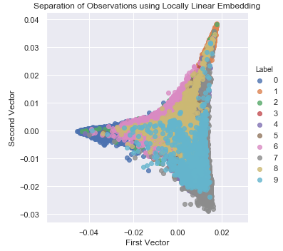
Figure 3-18. Separation of observations using LLE

t-Distributed Stochastic Neighbor Embedding (t-SNE)

t-distributed stochastic neighbor embedding (t-SNE) is a non-linear dimensionality reduction technique for visualizing high-dimensional data. t-SNE accomplishes this by modeling each high-dimensional point into a two or three-dimensional space, where similar points are modeled close to each other and dissimilar points are modeled farther away.¹²

It does this by constructing two probability distributions, one over pairs of points in the high-dimensional space and another over pairs of points in the low-dimensional space such that similar points have a high probability and dissimilar points have a lower probability. Specifically, t-SNE minimizes the Kullback-Leibler divergence between the two probability distributions.¹³

In real world applications of t-SNE, it is best to use another dimensionality reduction technique - such as PCA as we do here - to reduce the number of dimensions before applying t-SNE. By applying another form of dimensionality reduction first, we reduce the noise in the features that are fed into t-SNE and speed up the computation of the algorithm.

# t-SNE
from sklearn.manifold import TSNE

n_components = 2
learning_rate = 300
perplexity = 30
early_exaggeration = 12
init = 'random'
random_state = 2018

tSNE = TSNE(n_components=n_components, learning_rate=learning_rate, \
            perplexity=perplexity, early_exaggeration=early_exaggeration, \
            init=init, random_state=random_state)

X_train_tSNE = tSNE.fit_transform(X_train_PCA.loc[:5000,:9])
X_train_tSNE = pd.DataFrame(data=X_train_tSNE, index=train_index[:5001])

scatterPlot(X_train_tSNE, y_train, "t-SNE")

Figure 3-19 shows the two-dimensional scatter plot from t-SNE.

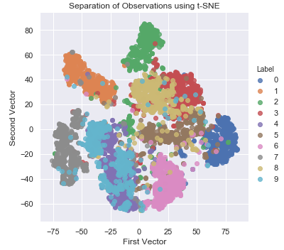
Figure 3-19. Separation of observations using t-SNE

Other Dimensionality Reduction Methods

We have covered both linear and non-linear forms of dimensionality reduction. Now, we will move to methods that do not rely on any sort of geometry or distance metric.

Dictionary Learning

One such method is dictionary learning, which learns the sparse representation of the original data. The resulting matrix is known as the dictionary, and the vectors in the dictionary are known as atoms. These atoms are simple, binary vectors, populated by zeros and ones. Each instance in the original data can be reconstructed as a weighted sum of these atoms.¹⁴

Assuming there are d features in the original data and n atoms in the dictionary, we can have a dictionary that is either undercomplete, where n < d, or overcomplete, where n > d. The undercomplete dictionary achieves dimensionality reduction, representing the original data with a fewer number of vectors, and this is what we will focus on.¹⁵

There is a mini-batch version of dictionary learning that we will apply to our dataset of digits. As with the other dimensionality reduction methods, we will set the number of components. We will also set the batch size and the number of iterations to perform the training.

Since we want to visualize the images using a two-dimensional scatterplot, we will learn a very dense dictionary, but, in practice, we would use a much sparser version.

# Mini-batch dictionary learning

from sklearn.decomposition import MiniBatchDictionaryLearning

n_components = 50
alpha = 1
batch_size = 200
n_iter = 25
random_state = 2018

miniBatchDictLearning = MiniBatchDictionaryLearning( \
                        n_components=n_components, alpha=alpha, \
                        batch_size=batch_size, n_iter=n_iter, \
                        random_state=random_state)

miniBatchDictLearning.fit(X_train.loc[:,:10000])
X_train_miniBatchDictLearning = miniBatchDictLearning.fit_transform(X_train)
X_train_miniBatchDictLearning = pd.DataFrame( \
    data=X_train_miniBatchDictLearning, index=train_index)

X_validation_miniBatchDictLearning = \
    miniBatchDictLearning.transform(X_validation)
X_validation_miniBatchDictLearning = \
    pd.DataFrame(data=X_validation_miniBatchDictLearning, \
    index=validation_index)

scatterPlot(X_train_miniBatchDictLearning, y_train, \
            "Mini-batch Dictionary Learning")

Figure 3-20 shows the two-dimensional scatter plot using dictionary learning.

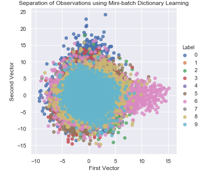
Figure 3-20. Separation of observations using dictionary learning

Independent Component Analysis

One common problem with unlabeled data is that there are many independent signals embedded together into the features we are given. Using independent component analysis (ICA), we can separate these blended signals into their individual components. After the separation is complete, we can reconstruct any of the original features by adding together some combination of the individual components we generate. ICA is commonly used in signal processing tasks (for example, to identify the individual voices in an audio clip of a busy coffeehouse).¹⁶

# Independent Component Analysis
from sklearn.decomposition import FastICA

n_components = 25
algorithm = 'parallel'
whiten = True
max_iter = 100
random_state = 2018

fastICA = FastICA(n_components=n_components, algorithm=algorithm, \
                  whiten=whiten, max_iter=max_iter, random_state=random_state)

X_train_fastICA = fastICA.fit_transform(X_train)
X_train_fastICA = pd.DataFrame(data=X_train_fastICA, index=train_index)

X_validation_fastICA = fastICA.transform(X_validation)
X_validation_fastICA = pd.DataFrame(data=X_validation_fastICA, \
                                    index=validation_index)

scatterPlot(X_train_fastICA, y_train, "Independent Component Analysis")

Figure 3-21 shows the two-dimensional scatter plot using independent component analysis.

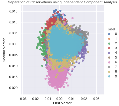
Figure 3-21. Separation of observations using independent component analysis

Conclusion

In this chapter, we introduced and explored a number of dimensionality reduction algorithms starting with linear methods such as principal component analysis and random projection. Then, we switched to non-linear methods - also known as manifold learning - such as Isomap, multi-dimensional scaling, locally linear embedding, and t-distributed neighbor embedding. We also covered non-distance-based methods such as dictionary learning and independent component analysis.

Dimensionality reduction captures the most salient information in a dataset in a small number of dimensions by learning the underlying structure of the data, and it does this without using any labels. By applying these algorithms to the MNIST digits dataset, we were able to meaningfully separate the images based on the digits they represented with just the top two dimensions.

This highlights the power of dimensionality reduction.

In Chapter 4, we will build an applied unsupervised learning solution using these dimensionality reduction algorithms. Specifically, we will revist the fraud detection problem introduced in chapter two and attempt to separate fraud transactions from normal ones without using any labels whatsoever.