
Consider a freight train carrying goods—some big and some small—across the country. Rather than put each item in its own railroad car, the little things are combined and put in one car and then separated at the far end. Compression does much the same thing. Given a set of numbers (some small and some large), you squeeze the small ones together for storage and then take them apart when you need to use them.
This book is built around implementing a delta compression routine. Given a set of N numbers, S
i
, i = 0, …, N − 1, the Steim compression method is to form a set of backward differences: δ
j
= S
j
− S
j−1, j = 1, …, N − 1.1
These differences (along with S
0, the first sample) are packed into a compressed string, where each difference may take up less space than the original sample. To uncompress the data, each difference must have an associated code c
i
indicating how many bytes were used for storing the difference: c
i
, i = 0, …, N − 1.
In this compression routine, the allowed sizes are 32 bits (4 bytes, or a long in Spin), 24 bits (3 bytes), 16 bits (2 bytes, or a word), and 8 bits (a byte). In more advanced compressors, 4-bit and 12-bit word lengths are allowed. I will leave that as an exercise for you!
2.1 Packing and Compressing Data
You can picture the memory impact of the compression with an example of four samples (7, 42, -12, 350) that must be compressed. Figure 2-1 shows the memory layout for these samples in panel (a) (from here out I will generally represent numbers in hexadecimal format and indicate that by prepending the number with 0x). In panel (b) I show the compressed and packed buffer layout with the 3-byte sample 0 storage and the subsequent differences stored. In panel (c) I show the compression coding.
It should be apparent that this compression method is best suited for time-series data where the mean of the numbers may be large but the standard deviation is small. Steim compression is most commonly used in data from seismographs (instruments that measure the ground motion to detect earthquakes). For much of the time, the seismographs are recording background noise, which has a small sample-to-sample variability. When an earthquake occurs, however, the seismograph output can and does change dramatically from one sample to the next. Figure 2-2 shows an example of a set of seismograms after a massive and destructive earthquake in Japan. All these data needs to be recorded and stored without any loss.
Figure 2-1
Compression
: (a) Samples are 4 bytes long but are packed into 1–3 bytes of differences of samples. (I know a priori that my numbers always fit in 3 bytes). (b) Sample 0 is stored as is; the difference between samples 1 and 0 is stored in the smallest number of bytes possible, and so on. (c) The length of storage is itself saved in the compression code array.
2.2 Specification
Input numbers must be valid 32-bit numbers, but the dynamic range of the samples is limited to 24 bits (that is the limit of our digitizer). Therefore, every sample can be represented and stored in at most 3 bytes. However, most programming languages prefer 4-byte numbers. Thus, on decompression, numbers should be 4 bytes long, with the uppermost byte sign extended from bit 23 (more on this later).
In the main cog
, I will define the following:
- nsamps: A long variable holding the number of samples N to process.
- sampsBuf: A long array holding the samples s i .
- packBuf: A byte array holding the compressed and packed differences δ i .
- codeBuf: A long array holding the compression code for each compressed sample.
- nCompr: A long variable holding the populated number of bytes in packBuf.
Here is what happens:
- 1.The compression program will compress nsamps numbers from the sampsBuf array and populate the output variables packBuf, codeBuf, and nCompr.
- 2.If nsamps is greater than the length of sampsBuf, return an error by setting ncompr to -1.
- 3.For sample zero:
- STEIM SHALL compress the first sample, s 0, by storing its bits 0 to 23 (the lower 3 bytes) into packBuf.
- STEIM SHALL store CODE24 in the lowest 2 bits of codeBuf.
- STEIM SHALL set nCompr to 3.
- (My digitizer has a 24-bit dynamic range, so all numbers fit within 3 or fewer bytes.)
- 4.For sample j (0 < j < N ) :
- STEIM will form the backward difference δ j = s j −s j−1 and determine whether the difference would fit completely within 1, 2, or 3 bytes and SHALL append those bytes to packBuf.
- STEIM SHALL increment nCompr by 1, 2, 3, according as the number of bytes needed for δ j .
- STEIM SHALL place the appropriate code (CODE08, CODE16, or CODE24) in comprBuf.
- 5.Finally, the decompression routine takes as input nsamps, packBuf, codeBuf, and nCompr and SHALL populate sampsBuf correctly.
2.3 Implementation
Now that we have a concise specification for the procedure, we will implement it in the following chapters (first in Spin, then in PASM, then in C, and finally in C and PASM). The way we will build up the implementations is similar in all cases. We will write a test for each of the previous bullets, and then we will write the code so that it passes the test.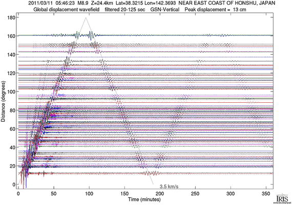
Figure 2-2
Seismograms
from around the world after the devastating Tohoku earthquake of March 2011 (magnitude 9). The lines show ground displacement at various seismographs ranging in distance from close to Japan (angular distance of 0 degrees) to the other side of the world from Japan (angular distance of 180 degrees). The horizontal axis is time after the earthquake occurs (in minutes). You can see the surface wave train travel around the world, back to Japan, and then repeat! In fact, the earth “rung like a bell” for hours after this event. Source:
http://ds.iris.edu/ds/nodes/dmc/specialevents/2011/03/11/tohoku-japan-earthquake/
.
Footnotes
1
This technique was popularized by Dr. JM Steim and has been implemented by the International Federation of Digital Seismograph Networks. The best description is in the SEED Reference Manual, “Standards for the Exchange of Earthquake Data,”
https://www.fdsn.org/seed_manual/SEEDManual_V2.4.pdf
. There is no published reference to Dr. Steim’s work.