Table of Contents for
Python Algorithms: Mastering Basic Algorithms in the Python Language, Second Edition
 Python Algorithms: Mastering Basic Algorithms in the Python Language, Second Edition
Published by
Apress, 2015
Python Algorithms: Mastering Basic Algorithms in the Python Language, Second Edition
Published by
Apress, 2015
- Cover
- Title
- Copyright
- Dedication
- Contents at a Glance
- Contents
- About the Author
- About the Technical Reviewer
- Acknowledgments
- Preface
- Chapter 1: Introduction
- Chapter 2: The Basics
- Chapter 3: Counting 101
- Chapter 4: Induction and Recursion … and Reduction
- Chapter 5: Traversal: The Skeleton Key of Algorithmics
- Chapter 6: Divide, Combine, and Conquer
- Chapter 7: Greed Is Good? Prove It!
- Chapter 8: Tangled Dependencies and Memoization
- Chapter 9: From A to B with Edsger and Friends
- Chapter 10: Matchings, Cuts, and Flows
- Chapter 11: Hard Problems and (Limited) Sloppiness
- Appendix A: Pedal to the Metal: Accelerating Python
- Appendix B: List of Problems and Algorithms
- Appendix C: Graph Terminology
- Appendix D: Hints for Exercises
- Index

Hard Problems and (Limited) Sloppiness
The best is the enemy of the good.
— Voltaire
This book is clearly about algorithmic problem solving. Until now, the focus has been on basic principles for algorithm design, as well as examples of important algorithms in many problem domains. Now, I’ll give you a peek at the flip side of algorithmics: hardness. Although it is certainly possible to find efficient algorithms for many important and interesting problems, the sad truth is that most problems are really hard. In fact, most are so hard that there’s little point in even trying to solve them. It then becomes important to recognize hardness, to show that a problem is intractable (or at least very likely so), and to know what alternatives there are to simply throwing your hands up.
There are three parts to this chapter. First, I’m going to explain the underlying ideas of one of the greatest unanswered questions in the world—and how it applies to you. Second, I’m going to build on these ideas and show you a bunch of monstrously difficult problems that you may very well encounter in one form or another. Finally, I’ll show you how following the wisdom of Voltaire, and relaxing your requirements a bit, can get you closer to your goals than might seem possible, given the rather depressing news in the first two parts of the chapter.
As you read the following, you may wonder where all the code has gone. Just to be clear, most of the chapter is about the kind of problems that are simply too hard. It is also about how you uncover that hardness for a given problem. This is important because it explores the outer boundaries of what our programs can realistically do, but it doesn’t really lead to any programming. Only in the last third of the chapter will I focus on (and give some code for) approximations and heuristics. These approaches will allow you to find usable solutions to problems that are too hard to solve optimally, efficiently, and in all generality. They achieve this by exploiting a loophole—the fact that in real life we may be content with a solution that is “good enough” along some or all of these three axes.
 Tip It might be tempting to skip ahead to the seemingly more meaty part of the chapter, where the specific problems and algorithms live. If you are to make sense of that, though, I strongly suggest giving the more abstract parts a go and at least skimming the chapter from the beginning to get an overview.
From Chapter 4, I’ve been discussing reductions every now and then. Mostly, I’ve been talking about reducing to a problem you know how to solve—either smaller instances of the problem you’re working on or a different problem entirely. That way, you’ve got a solution to this new, unknown problem as well, in effect proving that it’s easy (or, at least, that you can solve it). Near the end of Chapter 4, though, I introduced a different idea: reducing in the other direction to prove hardness. In Chapter 6, I used this idea to give a lower bound on the worst-case running time of any algorithm solving the convex hull problem. Now we’ve finally arrived at the point where this technique is completely at home. Defining complexity classes (and problem hardness) is, in fact, what reductions are normally used for in most textbooks. Before getting into that, though, I’d like to really hammer home how this kind of hardness proof works, at the fundamental level. The concept is pretty simple (although the proofs themselves certainly need not be), but for some reason, many people (myself included) keep getting it backward. Maybe—just maybe—the following little story can help you when you try to remember how it works.
Let’s say you’ve come to a small town where one of the main attractions is a pair of twin mountain peaks. The locals have affectionately called the two Castor and Pollux, after the twin brothers from Greek and Roman mythology. It is rumored that there’s a long-forgotten gold mine on the top of Pollux, but many an adventurer has been lost to the treacherous mountain. In fact, so many unsuccessful attempts have been made to reach the gold mine that the locals have come to believe it can’t be done. You decide to go for a walk and take a look for yourself.
After stocking up on donuts and coffee at a local roadhouse, you set off. After a relatively short walk, you get to a vantage point where you can see the mountains relatively clearly. From where you’re standing, you can see that Pollux looks like a really hellish climb—steep faces, deep ravines, and thorny brush all around it. Castor, on the other hand, looks like a climber’s dream. The sides slope gently, and it seems there are lots of handholds all the way to the top. You can’t be sure, but it seems like it might be a nice climb. Too bad the gold mine isn’t up there.
You decide to take a closer look and pull out your binoculars. That’s when you spot something odd. There seems to be a small tower on top of Castor, with a zip line down to the peak of Pollux. Immediately, you give up any plans you had to climb Castor. Why? (If you don’t immediately see it, it might be worth pondering for a bit.)1
Of course, we’ve seen the exact situation before, in the discussions of hardness in Chapters 4 and 6. The zip line makes it easy to get from Castor to Pollux, so if Castor were easy, someone would have found the gold mine already.2 It’s a simple contrapositive: If Castor were easy, Pollux would be too; Pollux is not easy, so Castor can’t be either. This is exactly what we do when we want to prove that a problem (Castor) is hard. We take something we know is hard (Pollux) and show that it’s easy to solve this hard problem using our new, unknown one (we uncover a zip line from Castor to Pollux).
As I’ve mentioned before, this isn’t so confusing in itself. It can be easy to confuse things when we start talking about it in terms of reductions, though. For example, is it obvious to you that we’re reducing Pollux to Castor here? The reduction is the zip line, which lets us use a solution to Castor as if it were a solution to Pollux. In other words, if you want to prove that problem X is hard, find some hard problem Y and reduce it to X.
Caution The zip line goes in the opposite direction of the reduction. It’s crucial that you don’t get this mixed up, or the whole idea falls apart. The term reduction here means basically “Oh, that’s easy, you just …” In other words, if you reduce A to B, you’re saying “You want to solve A? That’s easy, you just solve B.” Or in this case: “You want to scale Pollux? That’s easy, just scale Castor (and take the zip line).” In other words, we’ve reduced the scaling of Pollux to the scaling of Castor (and not the other way around).
A couple of things are worth noting here. First, we assume the zip line is easy to use. What if it wasn’t a zip line but a horizontal line that you had to balance across? This would be really hard—so it wouldn’t give us any information. For all we knew, people might easily get to the peak of Castor; they probably couldn’t reach the gold mine on Pollux anyway, so what do we know? The other is that reducing in the opposite direction tells us nothing either. A zip line from Pollux to Castor wouldn’t have impacted our estimate of Castor one bit. So, what if you could get to Castor from Pollux? You couldn’t get to the peak of Pollux anyway!
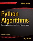
Consider the diagrams of Figure 11-1. The nodes represent problems, and the edges represent easy reductions (that is, they don’t matter, asymptotically). The thick line at the bottom is meant to illustrate “ground,” in the sense that unsolved problems are “up in the sky,” while solving them is equivalent to reducing them to nothing, or grounding them. The first image illustrates the case where an unknown problem u is reduced to a known, easy problem e. The fact that e is easy is represented by the fact that there’s an easy reduction from e to the ground. Linking u to e, therefore, gives us a path from u to the ground—a solution.
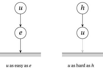
Figure 11-1. Two uses of reduction: reducing an unknown problem to an easy one or reducing a hard problem to an unknown one. In the latter case, the unknown problem must be as hard as the known one
Now look at the second image. Here, a known, hard problem is reduced to the unknown problem u. Can we have an edge from u to the ground (like the gray edge in the figure)? That would give us a path from h to the ground—but such a path cannot exist, or h wouldn’t be hard!
In the following, I’ll be using this basic idea not only to show that problems are hard but also to define some notions of hardness. As you may (or may not) have noticed, there is some ambiguity in the term hard here. It can basically have two different meanings:
- The problem is intractable—any algorithm solving it must be exponential.
- We don’t know whether the problem is intractable, but no one has ever been able to find a polynomial algorithm for it.
The first of these means that the problem is hard for a computer to solve, while the second means that it’s hard for people (and maybe computers as well). Take another look at the rightmost image in Figure 11-1. How would the two meaning of “hard” work here? Let’s take the first case: We know that h is intractable. It’s impossible to solve it efficiently. A solution to u (that is, a reduction to ground) would imply a solution to h, so no such solution can exist. Therefore, u must also be intractable.
The second case is a bit different—here the hardness involves a lack of knowledge. We don’t know if problem h is intractable, although we know that it seems difficult to find a solution. The core insight is still that if we reduce h to u, then u is at least as hard as h. If h is intractable, then so is u. Also, the fact that many people have tried to find a solution to h makes it seem less likely that we’ll succeed, which also means that it may be improbable that u is tractable. The more effort has been directed at solving h, the more astonishing it would be if u were tractable (because then so would h). This is, in fact, exactly the situation for a whole slew of practically important problems: We don’t know if they’re intractable, but most people are still highly convinced that they are. Let’s take a closer look at these rascal problems.
REDUCTION BY SUBPROBLEM
While the idea of showing hardness by using reductions can be a bit abstract and strange, there is one special case (or, in some ways, a different perspective) that can be easy to understand: if your problem has a hard subproblem, then the problem as a whole is (obviously) hard. In other words, if solving your problem means that you also have to solve a problem that is known to be hard, you’re basically out of luck. For example, if your boss asks you to create an antigravity hoverboard, you could probably do a lot of the work, such as crafting the board itself or painting on a nice pattern. However, actually solving the problem of circumventing gravity makes the whole endeavor doomed from the start.
So, how is this a reduction? It’s a reduction, because you can still use your problem to solve the hard subproblem. In other words, if you’re able to build an antigravity hoverboard, then your solution can (again, quite obviously) be used to circumvent gravity. The hard problem isn’t even really transformed, as in most reductions; it’s just embedded in a (rather irrelevant) context. Or consider the loglinear lower bound on the worst-case running time for general sorting. If you were to write a program that took in a set of objects, performed some operations on them, and then output information about the objects in sorted order, you probably couldn’t do any better than loglinear in the worst case.
But why “probably”? Because it depends on whether there’s a real reduction there. Could your program conceivably be used as a “sorting machine”? Would it be possible for me, if I could use your program as I wanted, to feed it objects that would let me sort any real numbers? If yes, then the bound holds. If no, then maybe it doesn’t. For example, maybe the sorting is based on integers that can be sorted using counting sort? Or maybe you actually create the sorting keys yourself, so the objects can be output in any order you please? The question of whether your problem is expressive enough—whether it can express the general sorting problem. This is, in fact, one of the key insights of this chapter: that problem hardness is a matter of expressiveness.
Not in Kansas Anymore?
As I wrote this chapter for the first edition, the excitement had only just started dying down around the Internet after a scientific paper was published online, claiming to prove to have solved the so-called P versus NP problem, concluding that P does not equal NP.3 Although the emerging consensus is that the proof is flawed, the paper created a tremendous interest—at least in computer science circles. Also, less credible papers with similar claims (or the converse, that P equals NP) keep popping up at regular intervals. Computer scientists and mathematicians have been working on this problem since the 1970s, and there’s even a million-dollar prize for the solution.4 Although much progress has been made in understanding the problem, no real solution seems forthcoming. Why is this so hard? And why is it so important? And what on Earth are P and NP?
The thing is, we don’t really know what kind of a world we’re living in. To use The Wizard of Oz as an analogy—we may think we’re living in Kansas, but if someone were to prove that P = NP, we’d most definitely not be in Kansas anymore. Rather, we’d be in some kind of wonderland on par with Oz, a world Russel Impagliazzo has christened Algorithmica.5 What’s so grand about Algorithmica, you say? In Algorithmica, to quote a well-known song, “You never change your socks, and little streams of alcohol come trickling down the rocks.” More seriously, life would be a lot less problematic. If you could state a mathematical problem, you could also solve it automatically. In fact, programmers no longer would have to tell the computer what to do—they’d only need to give a clear description of the desired output. Almost any kind of optimization would be trivial. On the other hand, cryptography would now be very hard because breaking codes would be so very, very easy.
The thing is, P and NP are seemingly very different beasts, although they’re both classes of problems. In fact, they’re classes of decision problems, problems that can be answered with yes or no. This could be a problem such as “Is there a path from s to t with a weight of at most w?” or “Is there a way of stuffing items in this knapsack that gives me a value of at least v?” The first class, P, is defined to consist of those problems we can solve in polynomial time (in the worst case). In other words, if you turn almost any of the problems we’ve looked at so far into a decision problem, the result would belong to P.
NP seems to have a much laxer definition6: It consists of any decision problems that can be solved in polynomial time by a “magic computer” called a nondeterministic Turing machine, or NTM. This is where the N in NP comes from—NP stands for “nondeterministically polynomial.” As far as we know, these nondeterministic machines are super-powerful. Basically, at any time where they need to make a choice, they can just guess, and by magic, they’ll always guess right. Sounds pretty awesome, right?
Consider the problem of finding the shortest path from s to t in a graph, for example. You already know quite a bit about how to do this with algorithms of the more … nonmagical kind. But what if you had an NTM? You’d just start in s and look at the neighbors. Which way should you go? Who knows—just take a guess. Because of the machine you’re using, you’ll always be right, so you’ll just magically walk along the shortest path with no detours. For such a problem as the shortest path in a DAG, for example, this might not seem like such a huge win. It’s a cute party trick, sure, but the running time would be linear either way.
But consider the first problem in Chapter 1: visiting all the towns of Sweden exactly once, as efficiently as possible. Remember how I said it took about 85 CPU-years to solve this problem with state-of-the-art technology a few years ago? If you had an NTM, you’d just need one computation step per town. Even if your machine were mechanical with a hand crank, it should finish the computation in a matter of seconds. This does seem pretty powerful, right? And magical?
Another way of describing NP (or, for that matter, nondeterministic computers) is to look at the difference between solving a problem and checking a solution. We already know what solving a problem means. If we are to check the solution to a decision problem, we’ll need more than a “yes” or “no”—we also require some kind of proof, or certificate (and this certificate is required to be of polynomial size). For example, if we want to know whether there is a path from s to t, a certificate might be the actual path. In other words, if you solved the problem and found that the answer was “yes,” you could use the certificate to convince me that this was true. To put it differently, if you managed to prove some mathematical statement, your proof could be the certificate.
The requirement, then, for a problem to belong to NP, is that I be able to check the certificate for any “yes” answers in polynomial time. A nondeterministic Turing machine can solve any such problem by simply guessing the certificate. Magic, right?
Well, maybe … You see, that’s the thing. We know that P is not magical—it’s full of problems we know very well how to solve. NP seems like a huge class of problems, and any machine that can solve all of them would be beyond this world. The thing is, in Algorithmica, there is such a thing as an NTM. Or, rather, our quite ordinary, humdrum computers (deterministic Turing machines) would turn out to be just as powerful. They had the magic in them all along! If P = NP, we could solve any (decision) problem that had a practical (verifiable) solution.
Meanwhile, Back in Kansas …
All right, Algorithmica is a magical world, and it would be totally awesome if we turned out to be living in it—but chances are, we’re not. In all likelihood, there is a very real difference between finding a proof and checking it—between solving a problem and simply guessing the right solution every time. So if we’re still in Kansas, why should we care about all of this?
Because it gives us a very useful notion of hardness. You see, we have a bunch of mean-spirited little beasties that form a class called NPC. This stands for “NP-complete,” and these are the hardest problems in all of NP. More precisely, each problem in NPC is at least as hard as every other problem in NP. We don’t know if they’re intractable, but if you were to solve just one of these tough-as-nails problems, you would automatically have transported us all to Algorithmica! Although the world population might rejoice at not having to change its socks anymore, this isn’t a very likely scenario (which I hope the previous section underscored). It would be utterly amazing but seems totally unfeasible.
Not only would it be earth-shatteringly weird, but given the enormous upsides and the monumental efforts that have been marshaled to break just a single one of these critters, the four decades of failure (so far) would seem to bolster our confidence in the wager that you’re not going to be the one to succeed. At least not anytime soon. In other words, the NP-complete problems might be intractable (hard for computers), but they’ve certainly been hard for humans so far.

NP-Complete. General solutions get you a 50% tip. (http://xkcd.com/287)
But how does this all work? Why would slaying a single NPC monster bring all of NP crashing down into P and send us tumbling into Algorithmica? Let’s return to our reduction diagrams. Take a look at Figure 11-2. Assume, for now, that all the nodes represent problems in NP (that is, at the moment we’re treating NP as “the whole world of problems”). The left image illustrates the idea of completeness. Inside a class of problems, a problem c is complete if all problems in that class can “easily” be reduced to c.7 In this case, the class we’re talking about is NP, and reductions are “easy” if they’re polynomial. In other words, a problem c is NP-complete if (1) c itself is in NP, and (2) every problem in NP can be reduced to c in polynomial time.
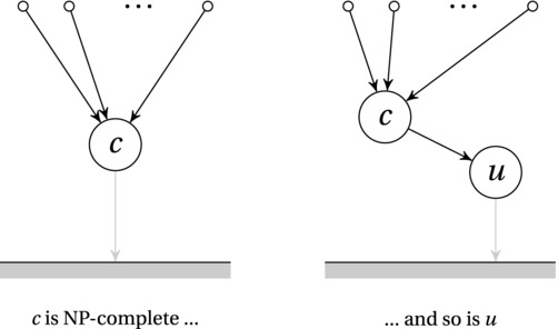
Figure 11-2. An NP-complete problem is a problem in NP that is at least as hard as all the others. That is, all the problems in NP can be reduced to it
The fact that every problem (in NP) can be reduced to these tough-nut problems means that they’re the hard core—if you can solve them, you can solve any problem in NP (and suddenly, we’re not in Kansas anymore). The figure should help make this clear: Solving c means adding a solid arrow from c to the ground (reducing it to nothing), which immediately gives us a path from every other problem in NP to the ground, via c.
We have now used reductions to define the toughest problems in NP, but we can extend this idea slightly. The right image in Figure 11-2 illustrates how we can use reductions transitively, for hardness proofs such as the ones we’ve been discussing before (like the one on the right in Figure 11-1, for example). We know that c is hard, so reducing it to u proves that u is hard. We already know how this works, but this figure illustrates a slightly more technical reason for why it is true in this case. By reducing c to u, we have now placed u in the same position that c was in originally. We already knew that every problem in NP could be reduced to c (meaning that it was NP-complete). Now we also know that every problem can be reduced to u, via c. In other words, u also satisfies the definition of NP-completeness—and, as illustrated, if we can solve it in polynomial time, we will have established that P = NP.
Now, so far I’ve only been talking about decision problems. The main reason for this is that it makes quite a few things in the formal reasoning (much of which I won’t cover here) a bit easier. Even so, these ideas are relevant for other kinds of problems, too, such as the many optimization problems we’ve been working with in this book (and will work with later in this chapter).
Consider, for example, the problem of finding the shortest tour of Sweden. Because it’s not a decision problem, it’s not in NP. Even so, it’s a very difficult problem (in the sense “hard for humans to solve” and “most likely intractable”), and just like anything in NP, it would suddenly be easy if we found ourselves in Algorithmica. Let’s consider these two points separately.
The term completeness is reserved for the hardest problems inside a class, so the NP-complete problems are the class bullies of NP. We can use the same hardness criterion for problems that might fall outside the class as well, though. That is, any problem that is at least as hard (determined by polynomial-time reduction) as any problem in NP, but that need not itself be in NP. Such problems are called NP-hard. This means that another definition of the class NPC, of NP-complete problems, is that it consists of all the NP-hard problems in NP. And, yes, finding the shortest route through a graph (such as through the towns of Sweden) is an NP-hard problem called the Traveling Salesman (or Salesrep) Problem, or often just TSP. I’ll get back to that problem a bit later.
About the other point: Why would an optimization problem such as this be easy if P = NP? There are some technicalities about how a certificate could be used to find the actual route, and so on, but let’s just focus on the difference between the yes-no nature of NP, and the numerical length we’re looking for in the TSP problem. To keep things simple, let’s say all edge weights are integers. Also, because P = NP, we can solve both the yes and no instances of our decision problems in polynomial time (see the sidebar “Asymmetry, Co-NP, and the Wonders of Algorithmica”). One way to proceed is then to use the decision problem as a black box and perform a binary search for the optimal answer.
For example, we can sum all the edge weights, and we get an upper limit C on the cost of the TSP tour, with 0 as a lower limit. We then tentatively guess that the minimum value is C/2 and solve the decision problem, “Is there a tour of length at most C/2?” We get a yes or a no in polynomial time and can then keep bisecting the upper or lower half of the value range. Exercise 11-1 asks you to show that the resulting algorithm is polynomial.
Tip This strategy of bisecting with a black box can be used in other circumstances as well, even outside the context of complexity classes. If you have an algorithm that lets you determine whether a parameter is large enough, you can bisect to find the right/optimal value, at the cost of a logarithmic factor. Quite cheap, really.
In other words, even though much of complexity theory focuses on decision problems, optimization problems aren’t all that different. In many contexts, you may hear people use the term NP-complete when what they really mean is NP-hard. Of course, you should be careful about getting things right, but whether you show a problem to be NP-hard or NP-complete is not all that crucial for the practical purpose of arguing its hardness. (Just make sure your reductions are in the right direction!)
ASYMMETRY, CO-NP, AND THE WONDERS OF ALGORITHMICA
The class of NP is defined asymmetrically. It consists of all decision problems whose yes instances can be solved in polynomial time with an NTM. Notice, however, that we don’t say anything about the no instances. So, for example, it’s quite clear that if there is a tour visiting each town in Sweden exactly once, an NTM would answer “yes” in a reasonable amount of time. If the answer is “no,” however, it may take its sweet time.
The intuition behind this asymmetry is quite accessible, really. The idea is that in order to answer “yes,” the NTM need only (by “magic”) find a single set of choices leading to a computation of that answer. In order to answer “no,” however, it needs to determine that no such computation exists. Although this does seem very different, we don’t really know if it is, though. You see, here we have another one of many “versus questions” in complexity theory: NP versus co-NP.
The class co-NP is the class of the complements of NP problems. For every “yes” answer, we now want “no,” and vice versa. If NP is truly asymmetric, then these two classes are different, although there is overlap between them. For example, all of P lies in their intersection, because both the yes and no instances in P can be solved in polynomial time with an NTM (and by a deterministic Turing machine, for that matter).
Now consider what would happen if an NP-complete problem FOO was found in the intersection of NP and co-NP. First of all, all problems in NP reduce to NPC, so this would mean that all of NP would be inside co-NP (because we could now deal with their complements, through FOO). Could there still be problems in co-NP outside of NP? Consider such a hypothetical problem, BAR. Its complement, co-BAR, would be in NP, right? But because NP was inside co-NP, co-BAR would also be in co-NP. That means that its complement, BAR, would be in NP. But, but, but … we assumed it to be outside of NP—a contradiction!
In other words, if we find a single NP-complete problem in the intersection of NP and co-NP, we’ll have shown that NP = co-NP, and the asymmetry has disappeared. As stated, all of P is in this intersection, so if P = NP, we’ll also have NP = co-NP. That means that in Algorithmica, NP is pleasantly symmetric.
Note that this conclusion is often used to argue that problems that are in the intersection of NP and co-NP are probably not NP-complete, because it is (strongly) believed that NP and co-NP are different. For example, no one has found a polynomial solution to the problem of factoring numbers, and this forms the basis of much of cryptography. Yet the problem is in both NP and co-NP, so most computer scientists believe that it’s not NP-complete.
But Where Do You Start? And Where Do You Go from There?
I hope the basic ideas are pretty clear now: The class NP consists of all decision problems whose “yes” answers can be verified in polynomial time. The class NPC consists of the hardest problems in NP; all problems in NP can be reduced to these in polynomial time. P is the set of problems in NP that we can solve in polynomial time. Because of the way the classes are defined, if there’s the least bit of overlap between P and NPC, we have P = NP = NPC. We’ve also established that if we have a polynomial-time reduction from an NP-complete problem to some other problem in NP, that second problem must also be NP-complete. (Naturally, all NP-complete problems can be reduced to each other in polynomial time; see Exercise 11-2.)
This has given us what seems to be a useful notion of hardness—but so far we haven’t even established that there exists such a thing as an NP-complete problem, let alone found one. How would we do that? Cook and Levin to the rescue!
In the early 1970s, Steven Cook proved that there is indeed such a problem, and a little later, Leonid Levin independently proved the same thing. They both showed that a problem called boolean satisfiability, or SAT, is NP-complete. This result has been named for them both and is now known as the Cook-Levin theorem. This theorem, which gives us our starting point, is quite advanced, and I can’t give you a full proof here, but I’ll try to outline the main idea. (A full proof is given by Garey and Johnson, for example; see the “References” section.)
The SAT problem takes a logical formula, such as (A or not B) and (B or C), and asks whether there is any way of making it true (that is, of satisfying it). In this case, of course, there is. For example, we could set A = B = True. To prove that this is NP-complete, consider an arbitrary problem FOO in NP and how you’d reduce it to SAT. The idea is to first construct an NTM that will solve FOO in polynomial time. This is possible by definition (because FOO is in NP). Then, for a given instance bar of FOO (that is, for a given input to the machine), you’d construct (in polynomial time) a logical formula (of polynomial size) expressing the following:
- The input to the machine was bar.
- The machine did its job correctly.
- The machine halts and answers “yes.”
The tricky part is how you’d express this using Boolean algebra, but once you do, it seems clear that the NTM is, in fact, simulated by the SAT problem given by this logical formula. If the formula is satisfiable—that is, if (and only if) we can make it true by assigning truth values to the various variables (representing, among other things, the magical choices made by the machine), then the answer to the original problem should be “yes.”
To recap, the Cook-Levin theorem says that SAT is NP-complete, and the proof basically gives you a way of simulating NTMs with SAT problems. This holds for the basic SAT problem and its close relative, Circuit-SAT, where we use a logical (digital) circuit, rather than a logical formula.
One important idea here is that all logical formulas can be written in what’s called conjunctive normal form (CNF), that is, as a conjunction (a sequence of ands) of clauses, where each clause is a sequence of ors. Each occurrence of a variable can be either of the form A or its negation, not A. The formulas may not be in CNF to begin with, but they can be transformed automatically (and efficiently). Consider, for example, the formula A and (B or (C and D)). It is entirely equivalent with this other formula, which is in CNF: A and (B or C) and (B or D).
Because any formula can be rewritten efficiently to a (not too large) CNF version, it should not come as a surprise that CNF-SAT is NP-complete. What’s interesting is that even if we restrict the number of variables per clause to k and get the so-called k-CNF-SAT (or simply k-SAT) problem, we can still show NP-completeness as long as k > 2. You’ll see that many NP-completeness proofs are based on the fact that 3-SAT is NP-complete.
IS 2-SAT NP-COMPLETE? WHO KNOWS …
When working with complexity classes, you need to be aware of special cases. For example, variations of the knapsack problem (or subset sum, which you’ll encounter in a bit) are used for encryption. The thing is, many cases of the knapsack problem are quite easy to solve. In fact, if the knapsack capacity is bounded by a polynomial (as a function of the item count), the problem is in P (see Exercise 11-3). If one is not careful when constructing the problem instances, the encryption can be quite easy to break.
We have a similar situation with k-SAT. For k ≥3, this problem is NP-complete. For k =2, though, it can be solved in polynomial time. Or consider the longest path problem. It’s NP-hard in general, but if you happen to know that your graph is a DAG, you can solve it in linear time. Even the shortest path problem is, in fact, NP-hard in the general case. The solution here is to assume the absence of negative cycles.
If you’re not working with encryption, this phenomenon is good news. It means that even if you’ve encountered a problem whose general form is NP-complete, it might be that the specific instances you need to deal with are in P. This is an example of what you might call the instability of hardness. Tweaking the requirements of your problem slightly can make a huge difference, making an intractable problem tractable, or even an undecidable problem (such as the halting problem) decidable. This is the reason why approximation algorithms (discussed later) are so useful.
Does this mean that 2-SAT is not NP-complete? Actually, no. Drawing this conclusion is an easy trap to fall into. This is true only if P ≠ NP because otherwise all problems in P are NP-complete. In other words, our NP-completeness proof fails for 2-SAT, and we can show it’s in P, but we do not know that it’s not in NPC.
Now we have a place to start: SAT and its close friends, Circuit SAT and 3-SAT. There are still lots of problems to examine, though, and replicating the feat of Cook and Levin seems a bit daunting. How, for example, would you show that every problem in NP could be solved by finding a tour through a set of towns?
This is where we (finally) get to start working with reductions. Let’s look at one of the rather simple NP-complete problems, that of finding a Hamilton cycle. I already touched upon this problem in Chapter 5 (in the sidebar “Island-Hopping in Kaliningrad”). The problem is to determine whether a graph with n nodes has a cycle of length n; that is, can you visit each node exactly once and return to your starting point, following the edges of the graph?
This doesn’t immediately look as expressive as the SAT problem—there we had access to the full language of propositional logic, after all—so encoding NTMs seems like a bit much. As you’ll see, it’s not. The Hamilton cycle problem is every bit as expressive as the SAT problem. What I mean by this is that there is a polynomial-time reduction from SAT to the Hamilton cycle problem. In other words, we can use the machinery of the Hamilton cycle problem to create a SAT solving machine!
I’ll walk you through the details, but before I do, I’d like to ask you to keep the big picture in the back of your mind: the general idea of what we’re doing is that we’re treating one problem as a sort of machine, and we’re almost programming that machine to solve a different problem. The reduction, then, is the metaphorical programming. With that in mind, let’s see how we can encode Boolean formulas as graphs so that a Hamilton cycle would represent satisfaction …
To keep things simple, let’s assume that the formula we want to satisfy is in CNF form. We can even assume 3-SAT (although that’s not really necessary). That means we have a series of clauses we need to satisfy, and in each of these, we need to satisfy at least one of the elements, which can be variables (such as A) or their negations (not A). Truth needs to be represented by paths and cycles, so let’s say we encode the truth value of each variable as a direction of a path.
This idea is illustrated in Figure 11-3. Each variable is represented by a single row of nodes, and these nodes are chained together with antiparallel edges so that we can move from left to right or from right to left. One direction (say, left to right) signifies that the variable is set to true, while the other direction means false. The number of nodes is immaterial, as long as we have enough.8
Figure 11-3. A single “row,” representing the variable A the Boolean expression we’re trying to satisfy. If the cycle passes through from left to right, the variable is true; otherwise, it’s false
Before we start trying to encode the actual formula, we want to force our machine to set each variable to exactly one of the two possible logical values. That is, we want to make sure that any Hamilton cycle will pass through each row (with the direction giving us the truth value). We also have to make sure the cycle is free to switch direction when going from one row to the next, so the variables can be assigned independently of each other. We can do this by connecting each row to the next with two edges, at the anchor points at either end (highlighted in Figure 11-3), as shown in Figure 11-4.
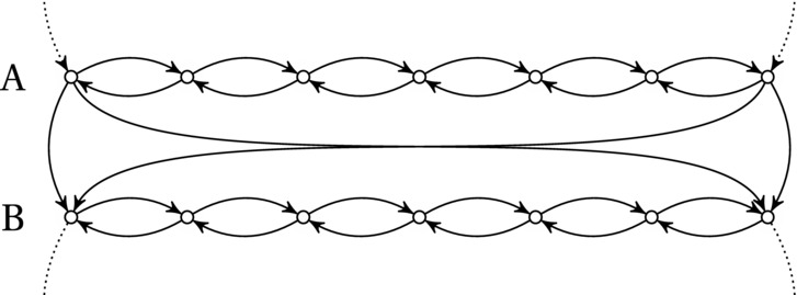
Figure 11-4. The rows are linked so the Hamilton cycle can maintain or switch its direction when going from one variable to the next, letting A and B be true or false, independently of each other
If we have only a set of rows connected as shown in Figure 11-4, there will be no Hamilton cycle in the graph. We can pass only from one row to the next and have no way of getting up again. The final touch to the basic row structure, then, is to add one source node s at the top (with edges to the left and right anchors of the first row) and a sink node t at the bottom (with edges from the left and right anchors of the last row) and then to add an edge from t to s.
Before moving on, you should convince yourself that this structure really does what we want it to. For k variables, the graph we have constructed so far will have 2k different Hamilton cycles, one for each possible assignment of truth values to the variables, with the truth values represented by the cycle going left or right in a given row.
Now that we’ve encoded the idea of assigning truth values to a set of logical variables in our Hamilton machine, we just need a way of encoding the actual formula involving these variables. We can do that by introducing a single node for each clause. A Hamilton cycle will then have to visit each of these exactly one time. The trick is to hook these clause nodes onto our existing rows to make use of the fact that the rows already encode truth values. We set things up so that the cycle can take a detour from the path, via the clause node, but only if it’s going in the right direction. So, for example, if we have the clause (A or not B), we’ll add a detour to the A row that requires the cycle to be going left to right, and we add another detour (via the same clause node) to the B row, but this time from right to left (because of the not). The only thing we need to watch out for is that no two detours can be linked to the rows in the same places—that’s why we need to have multiple nodes in each row, so we have enough for all the clauses. You can see how this would work for our example in Figure 11-5.
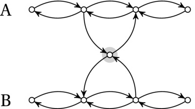
Figure 11-5. Encoding the clause (A or not B) using a clause node (highlighted), and adding detours requiring A to be true (left to right) and B to be false (right to left) in order to satisfy the clause (that is, visit the node)
After encoding the clauses in this way, each clause can be satisfied as long as at least one of its variables has the right truth value, letting it take a detour through the clause node. Because a Hamilton cycle must visit every node (including every clause node), the and-part of the formula is satisfied. In other words, the logical formula is satisfiable if and only if there is a Hamilton cycle in the graph we’ve constructed. This means that we have successfully reduced SAT (or, more specifically, CNF-SAT) to the Hamilton cycle problem, thereby proving the latter to be NP-complete! Now, was that so hard?
All right, so it was kind of hard. At least thinking of something like this yourself would be pretty challenging. Luckily, a lot of NP-complete problems are a lot more similar than SAT and the Hamilton cycle problem, as you’ll see in the following text.
A NEVERENDING STORY
There’s more to this story. There’s actually so much more to this story, you wouldn’t believe it. Complexity theory is a field of its own, with tons of results, not to mention complexity classes. (For a glimpse of the diversity of classes that are being studied, you could visit The Complexity Zoo, https://complexityzoo.uwaterloo.ca.)
One of the formative examples of the field is a problem that is much harder than the NP-complete ones: Alan Turing’s halting problem (mentioned in Chapter 4). It simply asks you to determine whether a given algorithm will terminate with a given input. To see why this is actually impossible, imagine you have a function halt that takes a function and an input as its parameters so that halt(A, X) will return true if A(X) terminates and false otherwise. Now, consider the following function:
def trouble(A):
while halt(A, A): pass
The call halt(A, A) determines whether A halts when applied to itself. Still comfortable with this? What happens if you evaluate trouble(trouble)? Basically, if it halts, it doesn’t, and if it doesn’t, it does … We have a paradox (or a contradiction), meaning that halt cannot possibly exist. The halting problem is undecidable. In other words, solving it is impossible.
But you think impossible is hard? As a great boxer once said, impossible is nothing. There is, in fact, such a thing as highly undecidable, or “very impossible.” For an entertaining introduction to these things, I recommend David Harel’s Computers Ltd: What They Really Can’t Do.
A Ménagerie of Monsters
In this section, I’ll give you a brief glimpse of a few of the thousands of known NP-complete problems. Note that the descriptions here serve two purposes at once. The first, and most obvious, purpose is to give you an overview of lots of hard problems so that you can more easily recognize (and prove) hardness in whatever problems you may come across in your programming. I could have given you that overview by simply listing (and briefly describing) the problems. However, I’d also like to give you some examples of how hardness proofs work, so I’m going to describe the relevant reductions throughout this section.
The problems in this section are mostly about selecting subsets. This is a kind of problem you can encounter in many settings. Perhaps you’re trying to choose which projects to finish within a certain budget? Or pack different-sized boxes into as few trucks as possible? Or perhaps you’re trying to fill a fixed set of trucks with a set of boxes that will give you as much profit as possible? Luckily, many of these problems have rather efficient solutions in practice (such as the pseudopolynomial solutions to the knapsack problems in Chapter 8 and the approximations discussed later in this chapter), but if you want a polynomial algorithm, you’re probably out of luck.9
Note Pseudopolynomial solutions are known for only some NP-hard problems. In fact, for many NP-hard problems, you can’t find a pseudopolynomial solution unless P = NP. Garey and Johnson call these NP-complete in the strong sense. (For more details, see Section 4.2 in their book, Computers and Intractability.)
The knapsack problem should be familiar by now. I discussed it with a focus on the fractional version in Chapter 7, and in Chapter 8 we constructed a pseudopolynomial solution using dynamic programming. In this section, I’ll have a look at both the knapsack problem itself and a few of its friends.
Let’s start with something seemingly simple,10 the so-called partition problem. It’s really innocent-looking—it’s just about equitable distribution. In its simplest form, the partition problem asks you to take a list of numbers (integers, say) and partition it into two lists with equal sums. Reducing SAT to the partition problem is a bit involved, so I’m just going to ask you to trust me on this one (or, rather, see the explanation of Garey and Johnson, for example).
Moving from the partition problem to others is easier, though. Because there’s seemingly so little complexity involved, using other problems to simulate the partition problem can be quite easy. Take the problem of bin packing, for example. Here we have a set of items with sizes in the range from 0 to k, and we want to pack them into bins of size k. Reducing from the partition problem is quite easy: We just set k to half the sum of the numbers. Now if the bin packing problem manages to cram the numbers into two bins, the answer to the partition problem is yes; otherwise, the answer is no. This means that the bin packing problem is NP-hard.
Another well-known problem that is simple to state is the so-called subset sum problem. Here you once again have a set of numbers, and you want to find a subset that sums to some given constant, k. Once again, finding a reduction is easy enough. For example, we can reduce from the partition problem, by (once again) setting k to half the sum of the numbers. A version of the subset sum problem locks k to zero—the problem is still NP-complete, though (Exercise 11-4).
Now, let’s look at the actual (integral, nonfractional) knapsack problem. Let’s deal with the 0-1 version first. We can reduce from the partition problem again, if we want, but I think it’s easier to reduce from subset sum. The knapsack problem can also be formulated as a decision problem, but let’s say we’re working with the same optimization version we’ve seen before: We want to maximize the sum of item values, while keeping the sum of item sizes below our capacity. Let each item be one of the numbers from the subset sum problem, and let both value and weight be equal to that number.
Now, the best possible answer we could get would be one where we match the knapsack capacity exactly. Just set the capacity to k, and the knapsack problem will give us the answer we seek: Whether we can fill up the knapsack completely is equivalent to whether we can find a sum of k.
To round up this section, I’ll just briefly touch upon one of the most obviously expressive problems out there: integer programming. This is a version of the technique of linear programming, where a linear function is optimized, under a set of linear constraints. In integer programming, though, you also require the variables to take on only integral values—which breaks all existing algorithms. It also means that you can reduce from all kinds of problems, with these knapsack-style ones as an obvious example. In fact, we can show that 0-1 integer programming, which is special case, is NP-hard. Just let each item of the knapsack problem be a variable, which can take on the value of 0 or 1. You then make two linear functions over these, with the values and weights as coefficients, respectively. You optimize the one based on the values and constrain the one based on the weights to be below the capacity. The result will then give you the optimal solution to the knapsack problem.11
What about the unbounded integral knapsack? In Chapter 8, I worked out a pseudopolynomial solution, but is it really NP-hard? It does seem rather closely related to the 0-1 knapsack, for sure, but the correspondence isn’t really close enough that a reduction is obvious. In fact, this is a good opportunity to try your hand at crafting a reduction—so I’m just going to direct you to Exercise 11-5.
Cliques and Colorings
Let’s move on from subsets of numbers to finding structures in graphs. Many of these problems are about conflicts. For example, you may be writing a scheduling software for a university, and you’re trying to minimize timing collisions involving teachers, students, classes, and auditoriums. Good luck with that one. Or perhaps you’re writing a compiler, and you want to minimize the number of registers used by finding out which variables can share a register? As before, you may find acceptable solutions in practice, but you may not be able to optimally solve large instances in general.
I have talked about bipartite graphs several times already—graphs whose nodes can be partitioned into two sets so that all edges are between the sets (that is, no edges connect nodes in the same set). Another way of viewing this is as a two-coloring, where you color every node as either black or white (for example), but you ensure that no neighbors have the same color. If this is possible, the graph is bipartite.
Now what if you’d like to see whether a graph is tripartite, that is, whether you can manage a three-coloring? As it turns out, that’s not so easy. (Of course, a k-coloring for k > 3 is no easier; see Exercise 11-6.) Reducing 3-SAT to three-coloring is, in fact, not so hard. It is, however, a bit involved (like the Hamilton cycle proof, earlier in this chapter), so I’m just going to give you an idea of how it works.
Basically, you build some specialized components, or widgets, just like the rows used in the Hamilton cycle proof. The idea here is to first create a triangle (three connected nodes), where one represents true, one false, and one is a so-called base node. For a variable A, you then create a triangle consisting of one node for A, one for not A, and the third being the base node. That way, if A gets the same color as the true node, then not A will get the color of the false node, and vice versa.
At this point, a widget is constructed for each clause, linking the nodes for either A or not A to other nodes, including the true and false nodes, so that the only way to find a three-coloring is if one of the variable nodes (of the form A or not A) gets the same color as the true node. (If you play around with it, you’ll probably find ways of doing this. If you want the full proof, it can be found in several algorithm books, such as the one by Kleinberg and Tardos; see “References” in Chapter 1.)
Now, given that k-coloring is NP-complete (for k > 2), so is finding the chromatic number of a graph—how many colors you need. If the chromatic number is less than or equal to k, the answer to the k-coloring problem is yes; otherwise, it is no. This kind of problem may seem abstract and pretty useless, but nothing could be further from the truth. This is an essential problem for cases where you need to determine certain kinds of resource needs, both for compilers and for parallel processing, for example.
Let’s take the problem of determining how many registers (a certain kind of efficient memory slots) a code segment needs. To do that, you need to figure out which variables will be used at the same time. The variables are nodes, and any conflicts are represented by edges. A conflict simply means that two variables are (or may be) used at the same time and therefore can’t share a register. Now, finding the smallest number of registers that can be used is equivalent to determining the chromatic number of this graph.
A close relative of the k-coloring is the so-called clique cover problem (also known as partitioning into cliques). A clique is, as you may recall, simply a complete graph, although the term is normally used when referring to a complete subgraph. In this case, we want to split a graph into cliques. In other words, we want to divide the nodes into several (nonoverlapping) sets so that within each set, every node is connected to every other. I’ll show you why this is NP-hard in a minute, but first, let’s have a closer look at cliques.
Simply determining whether a graph has a clique of a given size is NP-complete. Let’s say you’re analyzing a social network and you want to see whether there’s a group of k people, where every person is friends with every other. Not so easy … The optimization version, max-clique, is at least as hard, of course. The reduction from 3-SAT to the clique problem once again involves creating a simulation of logical variables and clauses. The idea here is to use three nodes for each clause (one for each literal, whether it be a variable or its negation) and then add edges between all nodes representing compatible literals, that is, those that can be true at the same time. (In other words, you add edges between all nodes except between a variable and its negation, such as A and not A.)
You do not, however, add edges inside a clause. That way, if you have k clauses and you’re looking for a clique of size k, you’re forcing at least one node from each clause to be in the clique. Such a clique would then represent a valid assignment of truth values to the variables, and you’d have solved 3-SAT by finding a clique. (Cormen et al. give a detailed proof; see “References” in Chapter 1.)
The clique problem has a very close relative—a yin to its yang, if you will—called the independent set problem. Here, the challenge is to find a set of k independent nodes (that is, nodes that don’t have any edges to each other). The optimization version is to find the largest independent set in the graph. This problem has applications to scheduling resources, just like graph coloring. For example, you might have some form of traffic system where various lanes in an intersection are said to be in conflict if they can’t be in use at the same time. You slap together a graph with edges representing conflicts, and the largest independent set will give you the largest number of lanes that can be in use at any one time. (More useful in this case, of course, would be to find a partition into independent sets; I’ll get back to that.)
Do you see the family resemblance to clique? Right. It’s exactly the same, except that instead of edges, we now want the absence of edges. To solve the independent set problem, we can simply solve the clique problem on the complement of the graph—where every edge has been removed and every missing edge has been added. (In other words, every truth value in the adjacency matrix has been inverted.) Similarly, we can solve the clique problem using the independent set problem—so we’ve reduced both ways.
Now let’s return to the idea of a clique cover. As I’m sure you can see, we might just as well look for an independent set cover in the complement graph (that is, a partitioning of the nodes into independent sets). The point of the problem is to find a cover consisting of k cliques (or independent sets), with the optimization version trying to minimize k. Notice that there are no conflicts (edges) inside an independent set, so all nodes in the same set can receive the same color. In other words, finding a k-clique-partition is essentially equivalent to finding a k-coloring, which we know is NP-complete. Equivalently, both optimization versions are NP-hard.
Another kind of cover is a vertex (or node) cover, which consists of a subset of the nodes in the graph and covers the edges. That is, each edge in the graph is incident to at least one node in the cover. The decision problem asks you to find a vertex cover consisting of at most k nodes. What we’ll see in a minute is that this happens exactly when the graph has an independent set consisting of at least n-k nodes, where n is the total number of nodes in the graph. This gives us a reduction that goes both ways, just like the one between cliques and independent sets.
The reduction is straightforward enough. Basically, a set of nodes is a vertex cover if and only if the remaining nodes form an independent set. Consider any pair of nodes that are not in the vertex cover. If there were an edge between them, it would not have been covered (a contradiction), so there cannot be an edge between them. Because this holds for any pair of nodes outside the cover, these nodes form an independent set. (A single node would work on its own, of course.)
The implication goes the other way as well. Let’s say you have an independent set—do you see why the remaining nodes must form a vertex cover? Of course, any edge not connected to the independent set will be covered by the remaining nodes. But what if an edge is connected to one of your independent nodes? Well, its other end can’t be in the independent set (those nodes aren’t connected), and that means that the edge is covered by an outside node. In other words, the vertex cover problem is NP-complete (or NP-hard, in its optimization version).
Finally, we have the set covering problem, which asks you to find a so-called set cover of size at most k (or, in the optimization version, to find the smallest one). Basically, you have a set S and another set F, consisting of subsets of S. The union of all the sets in F is equal to S. You’re trying to find a small subset of F that covers all the elements of S. To get an intuitive understanding of this, you can think of it in terms of nodes and edges. If S were the nodes of a graph, and F, the edges (that is, pairs of nodes), you’d be trying to find the smallest number of edges that would cover (be incident to) all the nodes.
Caution The example used here is the so-called edge cover problem. Although it’s a useful illustration of the set covering problem, you should not conclude that the edge cover problem is NP-complete. It can, in fact, be solved in polynomial time.
It should be easy enough to see that the set covering problem is NP-hard, because the vertex cover problem is basically a special case. Just let S be the edges of a graph and F consist of the neighbor sets for every node, and you’re done.
Paths and Circuits
This is our final group of beasties—and we’re drawing near to the problem that started the book. This material mainly has to do with navigating efficiently, when there are requirements on locations (or states) you have to pass through. For example, you might try to work out movement patterns for an industrial robot, or the layout of some kinds of electronic circuits. Once more you may have to settle for approximations or special cases. I’ve already shown how finding a Hamilton cycle in general is a daunting prospect. Now let’s see if we can shake out some other hard path and circuit-related problems from this knowledge.
First, let’s consider the issue of direction. The proof I gave that checking for Hamilton cycles was NP-complete was based on using a directed graph (and, thus, finding a directed cycle). What about the undirected case? It might seem we lose some information, and the earlier proof doesn’t hold here. However, with some widgetry, we can simulate direction with an undirected graph!
The idea is to split every node in the directed graph into three, basically replacing it by a length-two path. Imagine coloring the nodes: You color the original node blue, but you add a red in-node and a green out-node. All directed in-edges now become undirected edges linked to the red in-node, and the out-edges are linked to the green out-node. Clearly, if the original graph had a Hamilton cycle, the new one will as well. The challenge is getting the implication the other way—we need “if and only if” for the reduction to be valid.
Imagine that our new graph does have a Hamilton cycle. The node colors of this cycle would be either “… red, blue, green, red, blue, green …” or “… green, blue, red, green, blue, red …” In the first case, the blue nodes will represent a directed Hamilton cycle in the original graph, as they are entered only through their in-nodes (representing the original in-edges) and left through out-nodes. In the second case, the blue nodes will represent a reverse directed Hamilton cycle—which also tells us what we need to know (that is, that we have a usable directed Hamilton cycle in the other direction).
So, now we know that directed and undirected Hamilton cycles are basically equivalent (see Exercise 11-8). What about the so-called Hamilton path problem? This is similar to the cycle problem, except you’re no longer required to end up where you started. Seems like it might be a bit easier? Sorry. No dice. If you can find a Hamilton path, you can use that to find a Hamilton cycle. Let’s consider the directed case (see Exercise 11-9 for the undirected case). Take any node v with both in- and out-edges. (If there is no such node, there can be no Hamilton cycle.) Split it into two nodes, v and v’, keeping all in-edges pointing to v and all out-edges starting at v’. If the original graph had a Hamilton cycle, the transformed one will have a Hamilton path starting at v’ and ending at v (we’ve basically just snipped the cycle at v, making a path). Conversely, if the new graph has a Hamilton path, it must start at v’ (because it has no in-edges), and, similarly, it must end at v. By merging these nodes back together, we get a valid Hamilton cycle in the original graph.
Note The “Conversely …” part of the previous paragraph ensures we have implication in both directions. This is important, so that both “yes” and “no” answers are correct when using the reduction. This does not, however, mean that I have reduced in both directions.
Now, perhaps you’re starting to see the problem with the longest path problem, which I’ve mentioned a couple of times. The thing is, finding the longest path between two nodes will let you check for the presence of a Hamilton path! You might have to use every pair of nodes as end points in your search, but that’s just a quadratic factor—the reduction is still polynomial. As we’ve seen, whether the graph is directed or not doesn’t matter, and adding weights simply generalizes the problem. (See Exercise 11-11 for the acyclic case.)
What about the shortest path? In the general case, finding the shortest path is exactly equivalent to finding the longest path. You just need to negate all the edge weights. However, when we disallow negative cycles in the shortest path problem, that’s like disallowing positive cycles in the longest path problem. In both cases, our reductions break down (Exercise 11-12), and we no longer know whether these problems are NP-hard. (In fact, we strongly believe they’re not because we can solve them in polynomial time.)
Note When I say we disallow negative cycles, I mean in the graph. There’s no specific ban on negative cycles in the paths themselves because they are assumed to be simple paths and therefore cannot contain any cycles at all, negative or otherwise.
Now, finally, I’m getting to the great (or, by now, perhaps not so great) mystery of why it was so hard to find an optimal tour of Sweden. As mentioned, we’re dealing with the traveling salesman problem, or TSP. There are a few variations of this problem (most of which are also NP-hard), but I’ll start with the most straightforward one, where you have a weighted undirected graph, and you want to find a route through all the nodes, so that the weight sum of the route is as small as possible. In effect, what we’re trying to do is finding the cheapest Hamilton cycle—and if we’re able to find that, we’ve also determined that there is a Hamilton cycle. In other words, TSP is just as hard.
Travelling Salesman Problem. What’s the complexity class of the best linear programming cutting-plane techniques? I couldn’t find it anywhere. Man, the Garfield guy doesn’t have these problems … (http://xkcd.com/399)
But there’s another common version of TSP, where the graph is assumed to be complete. In a complete graph, there will always be a Hamilton cycle (if we have at least three nodes), so the reduction doesn’t really work anymore. What now? Actually, this isn’t as problematic as it might seem. We can reduce the previous TSP version to the case where the graph must be complete by setting the edge weights of the superfluous edges to some very large value. If it’s large enough (more than the sum of the other weights), we will find a route through the original edges, if possible.
The TSP problem might seem overly general for many real applications, though. It allows completely arbitrary edge weights, while many route planning tasks don’t require such flexibility. For example, planning a route through geographical locations or the movement of a robot arm requires only that we can represent distances in Euclidean space.12 This gives us a lot more information about the problem, which should make it easier to solve—right? Again, sorry. No. Showing that Euclidean TSP is NP-hard is a bit involved, but let’s look at a more general version, which is still a lot more specific than the general TSP: the metric TSP problem.
A metric is a distance function d(a,b), which measures the distance between two points, a and b. This need not be a straight-line, Euclidean distance, though. For example, when working out flight paths, you might want to measure distances along geodesics (curved lines along the earth’s surface), and when laying out a circuit board, you might want to measure horizontal and vertical distance separately, adding the two (resulting in so-called Manhattan distance or taxicab distance). There are plenty of other distances (or distance-like functions) that qualify as metrics. The requirements are that they be symmetric, non-negative real-valued functions that yield a distance of zero only from a point to itself. Also, they need to follow the triangular inequality: d(a,c) ≤ d(a,b) + d(b,c). This just means that the shortest distance between two points is given directly by the metric—you can’t find a shortcut by going through some other points.
Showing that this is still NP-hard isn’t too difficult. We can reduce from the Hamilton cycle problem. Because of the triangular inequality, our graph has to be complete.13 Still, we can let the original edges get a weight of one, and the added edges, a weight of, say, two (still doesn’t break things). The metric TSP problem will give us a minimum-weight Hamilton cycle of our metric graph. Because such a cycle always consists of the same number of edges (one per node), it will consist of the original (unit-weight) edges if and only if there is a Hamilton cycle in the original, arbitrary graph.
Even though the metric TSP problem is also NP-hard, you will see in the next section that it differs from the general TSP problem in a very important way: We have polynomial approximation algorithms for the metric case, while approximating general TSP is itself an NP-hard problem.
When the Going Gets Tough, the Smart Get Sloppy
As promised, after showing you that a lot of rather innocent-looking problems are actually unimaginably hard, I’m going to show you a way out: sloppiness. I mentioned earlier the idea of “the instability of hardness,” that even small tweaks to the problem requirements can take you from utterly horrible to pretty nice. There are many kinds of tweaks you can do—I’m going to cover only two. In this section, I’ll show you what happens if you allow a certain percentage of sloppiness in your search for optimality; in the next section, we’ll have a look at the “fingers crossed” school of algorithm design.
Let me first clarify the idea of approximation. Basically, we’ll be allowing the algorithm to find a solution that may not be optimal, but whose value is at most a given percentage off. More commonly, this percentage is given as a factor, or approximation ratio. For example, for a ratio of 2, a minimization algorithm would guarantee us a solution at most twice the optimum, while a maximization problem would give us one at least half the optimum.14 Let’s see how this works, by returning to a promise I made back in Chapter 7.
What I said was that the unbounded integer knapsack problem can be approximated to within a factor of two using greed. As for exact greedy algorithms, designing the solution here is trivial (just use the same greedy approach as for fractional knapsack); the problem is showing that it’s correct. How can it be that, if we keep adding the item type with the highest unit value (that is, value-to-weight ratio), we’re guaranteed to achieve at least half the optimum value? How on Earth can we know this when we have no idea what the optimum value is?
This is the crucial point of approximation algorithms. We don’t know the exact ratio of the approximation to the optimum—we give only a guarantee for how bad it can get. This means that if we get an estimate on how good the optimum can get, we can work with that instead of the actual optimum, and our answer will still be valid. Let’s consider the maximization case. If we know that the optimum will never be greater than A and we know our approximation will never be smaller than B, we can be certain that the ratio of the two will never be greater than A/B.15
For the unbounded knapsack, can you think of some upper limit to the value you can achieve? Well, we can’t get anything better than filling the knapsack to the brim with the item type with the highest unit value (sort of like an unbounded fractional solution). Such a solution might very well be impossible, but we certainly can’t do better. Let this optimistic bound be A.
Can we give a lower bound B for our approximation, or at least say something about the ratio A/B? Consider the first item you add. Let’s say it uses up more than half the capacity. This means we can’t add any more of this type, so we’re already worse off than the hypothetical A. But we did fill at least half the knapsack with the best item type, so even if we stop right now, we know that A/B is at most 2. If we manage to add more items, the situation can only improve.
What if the first item didn’t use more than half the capacity?16 Good news, everyone: We can add another item of the same kind! In fact, we can keep adding items of this kind until we’ve used at least half the capacity, ensuring that the bound on the approximation ratio still holds.
There are tons and tons of approximation algorithms out there—with plenty of books about this topic alone. If you want to learn more about the topic, I suggest getting one of those (both The Design of Approximation Algorithms by Williamson and Shmoys and Approximation Algorithms by Vijay V. Vazirany are excellent choices). I will show you one particularly pretty algorithm, though, for approximating the metric TSP problem.
What we’re going to do is, once again, to find some kind of invalid, optimistic solution and then tweak that until we get a valid (but probably not optimal) solution. More specifically, we’re going to aim for something (not necessarily a valid Hamilton cycle) that has a weight of at most twice the optimum solution and then tweak and repair that something using shortcuts (which the triangle inequality guarantees won’t make things worse), until we actually get a Hamilton cycle. That cycle will then also be at most twice the length of the optimum. Sounds like a plan, no?
What, though, would be only a few shortcuts away from a Hamilton cycle and yet be at most twice the length of the optimum solution? We can start with something simpler: What’s guaranteed to have a weight that is no greater than the shortest Hamilton cycle? Something we know how to find? A minimum spanning tree! Just think about it. A Hamilton cycle connects all nodes, and the absolutely cheapest way of connecting all nodes is using a minimum spanning tree.
A tree is not a cycle, though. The idea of the TSP problem is that we’re going to visit every node, walking from one to the next. We could certainly visit every node following the edges of a tree, as well. That’s exactly what Trémaux might do, if he were a salesman (see Chapter 5).17 In other words, we could follow the edges in a depth-first manner, backtracking to get to other nodes. This gives us a closed walk of the graph but not a cycle (because we’re revisiting nodes and edges). Consider the weight of this closed walk, though. We’re walking along each edge exactly twice, so it’s twice the weight of the spanning tree. Let this be our optimistic (yet invalid) solution.
The great thing about the metric case is that we can skip the backtracking and take shortcuts. Instead of going back along edges we’ve already seen, visiting nodes we’ve already passed through, we can simply make a beeline for the next unvisited node. Because of the triangular inequality, we’re guaranteed that this won’t degrade our solution, so we end up with an approximation ratio bound of two! (This algorithm is often called the “twice around the tree” algorithm, although you could argue that the name doesn’t really make that much sense because we’re going around the tree only once.)
Implementing this algorithm might not seem entirely straightforward. It kinda is, actually. Once we have our spanning tree, all we need is to traverse it and avoid visiting nodes more than once. Just reporting the nodes as they’re discovered during a DFS would actually give us the kind of solution we want. You can find an implementation of this algorithm in Listing 11-1. You can find the implementation of prim in Listing 7-5.
Listing 11-1. The “Twice Around the Tree” Algorithm, a 2-Approximation for Metric TSP
from collections import defaultdict

def mtsp(G, r):                                 # 2-approx for metric TSP
    T, C = defaultdict(list), []                # Tree and cycle
    for c, p in prim(G, r).items():             # Build a traversable MSP
        T[p].append(c)                          # Child is parent's neighbor
    def walk(r):                                # Recursive DFS
        C.append(r)                             # Preorder node collection
        for v in T[r]: walk(v)                  # Visit subtrees recursively
    walk(r)                                     # Traverse from the root
    return C                                    # At least half-optimal cycle
There is one way of improving this approximation algorithm that is conceptually simple but quite complicated in practice. It’s called Christofides’ algorithm, and the idea is that instead of walking the edges of the tree twice, it creates a min-cost matching among the odd-degree nodes of the spanning tree.18 This means that you can get a closed walk by following the edges of the tree once, and the edges of the matching once (and then fixing the solution by adding shortcuts, as before). We already know that the spanning tree is no worse than the optimum cycle. It can also be shown that the weight of the minimum matching is no greater than half the optimum cycle (Exercise 11-15), so in sum, this gives us a 1.5-approximation, the best bound known so far for this problem. The problem is that the algorithm for finding a min-cost matching is pretty convoluted (it’s certainly a lot worse than finding a min-cost bipartite matching, as discussed in Chapter 10), so I’m not going to go into details here.
Given that we can find a solution for the metric TSP problem that is a factor of 1.5 away from the optimum, even though the problem is NP-hard, it may be a bit surprising that finding such an approximation algorithm—or any approximation within a fixed factor of the optimum—is itself an NP-hard problem for TSP in general (even if the TSP graph is complete). This is, in fact, the case for several problems, which means that we can’t necessarily rely on approximation as a practical solution for all NP-hard optimization problems.
To see why approximating TSP is NP-hard, we do a reduction from the Hamilton cycle problem to the approximation. You have a graph, and you want to find out whether it has a Hamilton cycle. To get the complete graph for the TSP problem, we add any missing edges, but we make sure we give them huge edge weights. If our approximation ratio is k, we make sure these edge weights are greater than km, where m is the number of edges in the original graph. Then an optimum tour of the new graph would be at most m if we could find a Hamilton tour of the original, and if we included even one of the new edges, we’d have broken our approximation guarantee. That means that if (and only if) there were a Hamilton cycle in the original graph, the approximation algorithm for the new one would find it—meaning that the approximation is at least as hard (that is, NP-hard).
Desperately Seeking Solutions
We’ve looked at one way that hardness is unstable—sometimes finding near-optimal solutions can be vastly easier than finding optimal ones. There is another way of being sloppy, though. You can create an algorithm that is basically a brute-force solution but that uses guesswork to try to avoid as much computation as possible. With a little luck, if the instance you’re trying to solve isn’t one of the really hard ones, you may actually be able to find a solution pretty quickly! In other words, the sloppiness here is not about the quality of the solution but about the running time guarantees.
This is a bit like with quicksort, which has a quadratic worst-case running time but which is loglinear in the average case, with very low constant factors. Much of the reasoning about hard problems deals with what guarantees we can give about the worst-case performance, but in practice, that may not be all we care about. In fact, even if we’re not in Russel Impagliazzo’s fantasy world, Algorithmica, we may be in one of his other worlds, which he calls Heuristica. Here, NP-hard problems are still intractable in the worst case, but they’re tractable in the average case. And even if this isn’t the case, it certainly is the case that by using heuristic methods, we can often solve problems that might seem impossible.
There are plenty of methods in this vein. The A* algorithm discussed in Chapter 9, for example, can be used to search through a space of solutions in order to find a correct or optimal one. There are also such heuristic search techniques as artificial evolution and simulated annealing (see “If You’re Curious …” later in this chapter). In this section, though, I’ll show you a really cool and actually pretty simple idea, which can be applied to hard problems such as those discussed in this chapter but which can also serve as a quick-and-dirty way of solving any kind of algorithmic problem, even ones for which there are polynomial solutions. This could be useful either because you can’t think of a custom algorithm or because your custom algorithm is too slow.
The technique is called branch and bound and is particularly well-known in the field of artificial intelligence. There’s even a special version of it (called alpha-beta pruning) used in programs playing games. (For example, if you have a chess program, chances are there’s some branch and bound going on inside it.) In fact, branch and bound is one of the main tools for solving NP-hard problems, including such general and expressive ones as integer programming. Even though this awesome technique follows a very straightforward schema, it can be hard to implement in a completely general fashion. Chances are, if you’re going to use it, you’ll have to implement a version that is customized to your problem.
Branch and bound, or B&B, is based on gradually building solutions, sort of like a lot of greedy algorithms (see Chapter 7). In fact, which new building block to consider is often chosen greedily, resulting in so-called best-first branch and bound. However, instead of fully committing to this new building block (or this way of extending the solution), all possibilities are considered. At the core, we’re dealing with a brute-force solution. The thing that can make it all work, though, is that whole avenues of exploration can be pruned away, by reasoning about how promising (or, rather, unpromising) they are.
To make this more concrete, let’s consider a specific example. In fact, let’s revisit one we’ve worked with in several ways before, the 0-1 knapsack problem. In 1967, Peter J. Kolesar published the paper “A branch and bound algorithm for the knapsack problem,” where he describes exactly this approach. As he puts it, “A branch and bound algorithm proceeds by repeatedly partitioning the class of all feasible solutions into smaller and smaller subclasses in such a way that ultimately an optimal solution is obtained.” These “classes” are what we get by constructing partial solutions.
For example, if we decide to include item x in our knapsack, we have implicitly constructed the class of all solutions including x. There is, of course, also the complement of this class, all solutions that do not include x. We will need to examine both of these classes, unless we can somehow reach the conclusion that one of them cannot contain the optimum. You can picture this as a tree-shaped state space, a concept mentioned in Chapter 5. Each node is defined by two sets: the items that are included in the knapsack, and the items that are excluded from it. Any remaining items are as yet undetermined.
In the root of this (abstract, implicit) tree structure, no objects are included or excluded, so all are undetermined. To expand a node into two child nodes (the branching part), we decide on one of the undecided objects and include it to get one child and exclude it to get the other. If a node has no undecided items, it’s a leaf, and we can get no further.
It should be clear that if we explore this tree fully, we will examine every possible combination of included and excluded objects (a brute-force solution). The whole idea of branch and bound algorithms is to add pruning to our traversal (just like in bisection and search trees), so we visit as little as possible of the search space. As for approximation algorithms, we introduce upper and lower bounds. For a maximization problem, we use a lower bound on the optimum (based on what we’ve found so far) and use an upper bound on the solutions in any given subtree (based on some heuristic).19 In other words, we’re comparing a conservative estimate of the optimum with an optimistic estimate of what we can find in a given subtree. If the conservative bound is better than the optimistic bound on what a subtree contains, that subtree cannot hold the optimum, and so it is pruned (the bounding part).
In the basic case, the conservative bound for the optimum is simply the best value we’ve found so far. It can be extremely beneficial to have this bound be as high as possible when the B&B starts running, so we might want to spend some time on that first. (For example, if we were looking for a metric TSP tour, which is a minimization problem, we could set the initial upper bound to the result of our approximation algorithm.) To keep things simple for our knapsack example, though, let’s just keep track of the best solution, starting out with a value of zero. (Exercise 11-16 asks you to improve on this.)
The only remaining conundrum is how to find an upper bound for a partial solution (representing a subtree of the search space). If we don’t want to lose the actual solution, this bound has to be a true upper bound; we don’t want to exclude a subtree based on overly gloomy predictions. Then again, we shouldn’t be too optimistic (“This might have infinite value! Yay!”) because then we’d never get to exclude anything. In other words, we need to find an upper bound that is as tight (low) as we can make it. One possibility (and the one used by Kolesar) is to pretend we’re dealing with the fractional knapsack problem and then use the greedy algorithm on that. This solution can never be worse than the actual optimum we’re looking for (Exercise 11-17), and it turns out it’s a pretty tight bound for practical purposes.
You can see one possible implementation of the 0-1 knapsack B&B in Listing 11-2. To keep things simple, the code calculates only the value of the optimum solution. If you want the actual solution structure (which items are included), you’ll need to add some additional bookkeeping. As you can see, instead of explicitly managing two sets for each node (included and excluded items), only the weight and value sums of items included so far are used, with a counter (m) indicating which items have been considered (in order). Each node is a generator, which will (when prompted) generate any promising children.
Note The nonlocal keyword, which is used in Listing 11-2, lets you modify a variable in a surrounding scope, just like global lets you modify the global scope. However, this feature was new in Python 3.0. If you want similar functionality in earlier Pythons, simply replace the initial sol = 0 by sol = [0] and later access the value using the expression sol[0] instead of just sol. (For more information, see PEP 3104, available at http://legacy.python.org/dev/peps/pep-3104.)
And the Moral of the Story Is …
All right. This chapter may not be the easiest one in the book, and it may not be entirely obvious how to use some of the topics here in your day-to-day coding. To clarify the main points of the chapter, I thought I’d try to give you some advice on what to do when a monster problem crosses your path.
- First, follow the first two pieces of problem solving advice in Chapter 4. Are you sure you really understand the problem? Have you looked everywhere for a reduction (for example, do you know of any algorithms that seem even remotely relevant)?
- If you’re stumped, look again for reductions, but this time from some known NP-hard problems, rather than to problems you know how to solve. If you find one, at least you know the problem is hard, so there’s no reason to beat yourself up.
- Consider the last bit of problem solving advice from Chapter 4: Are there any extra assumptions you can exploit to make the problem less monstrous? The longest path problem is NP-hard in general, but in a DAG, you can solve it easily.
- Can you introduce some slack? If your solution needn’t be 100 percent optimal, perhaps there is an approximation algorithm you can use? You could either design one or research the literature on the subject. If you don’t need polynomial worst-case guarantees, perhaps something like branch and bound could work?
Listing 11-2. Solving the Knapsack Problem with the Branch and Bound Strategy
from __future__ import division
from heapq import heappush, heappop
from itertools import count

def bb_knapsack(w, v, c):
    sol = 0                                     # Solution so far
    n = len(w)                                  # Item count

    idxs = list(range(n))
    idxs.sort(key=lambda i: v[i]/w[i],          # Sort by descending unit cost
              reverse=True)

    def bound(sw, sv, m):                       # Greedy knapsack bound
        if m == n: return sv                    # No more items?
        objs = ((v[i], w[i]) for i in idxs[m:]) # Descending unit cost order
        for av, aw in objs:                     # Added value and weight
            if sw + aw > c: break               # Still room?
            sw += aw                            # Add wt to sum of wts
            sv += av                            # Add val to sum of vals
        return sv + (av/aw)*(c-sw)              # Add fraction of last item

    def node(sw, sv, m):                        # A node (generates children)
        nonlocal sol                            # "Global" inside bb_knapsack
        if sw > c: return                       # Weight sum too large? Done
        sol = max(sol, sv)                      # Otherwise: Update solution
        if m == n: return                       # No more objects? Return
        i = idxs[m]                             # Get the right index
        ch = [(sw, sv), (sw+w[i], sv+v[i])]     # Children: without/with m
        for sw, sv in ch:                       # Try both possibilities
            b = bound(sw, sv, m+1)              # Bound for m+1 items
            if b > sol:                         # Is the branch promising?
                yield b, node(sw, sv, m+1)      # Yield child w/bound

    num = count()                               # Helps avoid heap collisions
    Q = [(0, next(num), node(0, 0, 0))]         # Start with just the root
    while Q:                                    # Any nodes left?
        _, _, r = heappop(Q)                    # Get one
        for b, u in r:                          # Expand it ...
            heappush(Q, (b, next(num), u))      # ... and push the children

    return sol                                  # Return the solution
If all else fails, you could implement an algorithm that seems reasonable and then use experiments to see whether the results are good enough. For example, if you’re scheduling lectures to minimize course collisions for students (a kind of problem that’s easily NP-hard), you may not need a guarantee that the result will be optimal, as long as the results are good enough.20
Summary
This chapter has been about hard problems and some of the things you can do to deal with them. There are many classes of (seemingly) hard problems, but the most important one in this chapter is NPC, the class of NP-complete problems. NPC forms the hard core of NP, the class of decision problems whose solutions can be verified in polynomial time—basically every decision problem of any real practical use. Every problem in NP can be reduced to every problem in NPC (or to any so-called NP-hard problem) in polynomial time, meaning that if any NP-complete problem can be solved in polynomial time, every problem in NP can be, as well. Most computer scientists find this scenario highly unlikely, although no proof as yet exists either way.
The NP-complete and NP-hard problems are legion, and they crop up in many contexts. This chapter gave you a taste of these problems, including brief proof sketches for their hardness. The basic idea for such proofs is to rely on the Cook-Levin theorem, which says that the SAT problem is NP-complete, and then to reduce in polynomial time either from that, or from some other problem we have already shown to be NP-complete or NP-hard.
The strategies hinted at for actually dealing with these hard problems are based on controlled sloppiness. Approximation algorithms let you control precisely how far your answer will be from the optimum, while heuristic search methods such as branch and bound guarantee you an optimal solution but can take an unspecified amount of time to finish.
If You’re Curious …
There are lots of books out there that deal with computational complexity, approximation algorithms, and heuristic algorithms; see the “References” section for some ideas.
One area that I haven’t touched upon at all is that of so-called metaheuristics, a form of heuristic search that gives few guarantees but that can be surprisingly powerful. For example, there is artificial evolution, with so-called genetic programming, or GP, as one of its most well-known techniques. In GP, you maintain a virtual population of structures, usually interpreted as little computer programs (although they could be Hamilton cycles in the TSP problem, for example, or whatever structure you’d like to build). In each generation, you evaluate these individual (for example, computing their length when solving the TSP problem). The most promising ones are allowed to have offspring—new structures in the next generation, based on the parents, but with some random modifications (either simple mutation, or even combinations of several parent structures). Other metaheuristic methods are based on how melted materials behave when cooled down slowly (simulated annealing), how you might search for things when avoiding areas where you’ve recently looked (tabu search), or even how a swarm of insect-like solutions might move around in the state space (particle swarm optimization).
Exercises
11-1. We’ve seen several cases where the running time of an algorithm depends on one of the values in the input, rather than the actual size of the input (for example, the dynamic programming solution to the 0-1 knapsack problem). In these cases, the running time has been called pseudopolynomial, and it has been exponential as a function of problem size. Why is bisecting for a specific integer value an exception to this?
11-2. Why can every NP-complete problem be reduced to every other?
11-3. If the capacity of the knapsack problem is bounded by a function that is polynomial in the number of items, the problem is in P. Why?
11-4. Show that the subset sum problem is NP-complete even if the target sum, k, is fixed at zero.
11-5. Describe a polynomial-time reduction from the subset sum problem with positive integers to the unbounded knapsack problem. (This can be a bit challenging.)
11-6. Why is a four-coloring, or any k-coloring for k > 3, no easier than a three-coloring?
11-7. The general problem of isomorphism, finding out whether two graphs have the same structure (that is, whether they’re equal if you disregard the labels or identities of the nodes), is not known to be NP-complete. The related problem of subgraph isomorphism is, though. This problem asks you to determine whether one graph has a subgraph that is isomorphic to another. Show that this problem is NP-complete.
11-8. How would you simulate the undirected Hamilton cycle problem using the directed version?
11-9. How would you reduce the undirected Hamilton cycle problem (directed or undirected) to the undirected Hamilton path problem?
11-10. How would you reduce the Hamilton path problem to the Hamilton cycle problem?
11-11. Why don’t the proofs given in this section let us conclude that finding the longest path in a DAG is NP-complete? Where do the reductions break down?
11-12. Why haven’t we shown that the longest path problem without positive cycles is NP-complete?
11-13. In the greedy 2-approximation for the unbounded knapsack problem, why can we be certain that we can fill more than half the knapsack (assuming that at least some objects will fit in it)?
11-14. Let’s say you have a directed graph and you want to find the largest subgraph without cycles (the largest sub-DAG, so to speak). You’ll measure the size in the number of edges involved. You think the problem seems a bit challenging, though, so you’ve decided that you’ll settle for a 2-approximation. Describe such an approximation.
11-15. In Christofides’ algorithm, why is there a matching of the odd-degree nodes with a total weight equal to at most half that of the optimum Hamilton cycle?
11-16. Devise some improvement on the starting-value for lower bound on the optimum in the branch and bound solution for the 0-1 knapsack.
11-17. Why is the greedy fractional solution never worse than the actual optimum in 0-1 knapsack?
11-18. Consider the optimization problem MAX-3-SAT (or MAX-3-CNF-SAT), where you’re trying to make as many of the clauses in a 3-CNF formula true. This is clearly NP-hard (because it can be used to solve 3-SAT), but there is a curiously effective and oddly simple randomized approximation algorithm for it: Just flip a coin for each variable. Show that in the average case, this is an 8/7-approximation (assuming that no clause contains both a variable and its negation).
11-19. In Exercises 4-3 and 10-8, you started building a system for selecting friends to invite to a party. You have a numerical compatibility with each guest, and you want to select a subset that gives you a highest possible sum of compatibilities. Some guests would come only if certain others were present, and you managed to accommodate this constraint. You realize, however, that some of the guests will refuse to come if certain others are present. Show that solving the problem suddenly got a lot harder.
11-20. You’re writing a system for parallel processing that distributes batch jobs to different processors in order to get all the work done as quickly as possible. You have the processing times for n jobs, and you are to divide these among m identical processors so that the final completion time is minimized. Show that this is NP-hard, and describe and implement an algorithm that solves the problem with approximation ratio 2.
11-21. Use the branch and bound strategy and write a program that finds an optimal solution to the scheduling problem in Exercise 11-20.
References
Arora, S. and Barak, B. (2009). Computational Complexity: A Modern Approach. Cambridge University Press.
Crescenzi, G. A., Gambosi, G., Kann, V., Marchetti-Spaccamela, A., and Protasi, M. (1999). Complexity and Approximation: Combinatorial Optimization Problems and Their Approximability Properties. Springer. Appendix online: ftp://ftp.nada.kth.se/Theory/Viggo-Kann/compendium.pdf.
Garey, M. R. and Johnson, D. S. (2003). Computers and Intractability: A Guide to the Theory of NP-Completeness. W. H. Freeman and Company.
Goldreich, O. (2010). P, NP, and NP-Completeness: The Basics of Computational Complexity. Cambridge University Press.
Harel, D. (2000). Computers Ltd: What They Really Can’t Do. Oxford University Press.
Hemaspaandra, L. A. and Ogihara, M. (2002). The Complexity Theory Companion. Springer.
Hochbaum, D. S., editor (1997). Approximation Algorithms for NP-Hard Problems. PWS Publishing Company.
Impagliazzo, R. (1995). A personal view of average-case complexity. In Proceedings of the 10th Annual Structure in Complexity Theory Conference (SCT ’95), pages 134–147. http://cseweb.ucsd.edu/~russell/average.ps.
Kolesar, P. J. (1967). A branch and bound algorithm for the knapsack problem. Management Science, 13(9):723–735. http://www.jstor.org/pss/2628089.
Vazirani, V. V. (2010). Approximation Algorithms. Springer.
Williamson, D. P. and Shmoys, D. B. (2011). The Design of Approximation Algorithms. Cambridge University Press. http://www.designofapproxalgs.com.
___________________
1You can assume that getting down from Pollux is easy enough. Perhaps there’s a water slide? And that all of this was built before Pollux got so impregnable. Perhaps there was a rockslide?
2“An economics professor and a student were strolling through the campus. ‘Look,’ the student cried, ‘there’s a $100 bill on the path!’ ‘No, you are mistaken,’ the wiser head replied. ‘That cannot be. If there were actually a $100 bill, someone would have picked it up.’” (From Compensation, by G. T. Milkovich and J. M. Newman.)
3Vinay Deolalikar. P is not equal to NP. August 6, 2010.
4http://www.claymath.org/millennium-problems
5Actually, Impagliazzo’s definition of Algorithmica also permits some slightly different scenarios.
6Note the “seems to.” We don’t really know whether P = NP, so the definition might actually be equivalent.
7Although I don’t make a big fuss about it here, the fact that such problems exist is actually pretty weird.
8We need to stick with a polynomial number of nodes, of course.
9Both for this section and the following two, you might want to try to show that the examples in the initial paragraphs are, in fact, NP-hard.
10To make it easier to follow the arguments in these sections, I’ll generally progress (using reductions) from seemingly simple problems to more expressive ones. In reality, of course, they’re all just as expressive (and hard)—but some problems hide this better than others.
11This paragraph is probably easier to understand if you already know a little bit about linear programming. If you didn’t quite catch all of it, don’t worry—it’s not really essential.
12Unless we want to take relativity or the curvature of the earth into account ...
13Any infinite distances would break it, unless it was completely without edges or consisted of only two nodes.
14Note that we always divide the larger of the two (optimum and approximation) by the smaller.
15For the minimization case, just reverse the logic, and consider the ratio B/A.
16Notice the use of “proof by cases” here. It’s a really useful technique.
17I’m guessing he’d think of something better, though.
18You might want to verify for yourself that the number of odd-degree nodes in any graph is even.
19If you were minimizing, the bounds would, of course, be swapped.
20And if you want to get fancy, you could always research some of the many heuristic search methods originating in the field of artificial intelligence, such as genetic programming and tabu search. See the “If You’re Curious ...” section for more.