Python Algorithms: Mastering Basic Algorithms in the Python Language, Second Edition

APPENDIX C

Graph Terminology

He offered a bet that we could name any person among earth’s one and a half billion inhabitants and through at most five acquaintances, one of which he knew personally, he could link to the chosen one.

— Frigyes Karinthy, Láncszemek¹

The following presentation is loosely based on the first chapters of Graph Theory by Reinhard Diestel and Digraphs by Bang-Jensen and Gutin, and on the appendixes of Introduction to Algorithms by Cormen et al. (Note that the terminology and notation may differ between books; it is not completely standardized.) If you think it seems like there’s a lot to remember and understand, you probably needn’t worry. Yes, there may be many new words ahead, but most of the concepts are intuitive and straightforward, and their names usually make sense, making them easier to remember.

So … A graph is an abstract network, consisting of nodes (or vertices), connected by edges (or arcs). More formally, we define a graph as a pair of sets, G = (V, E), where the node set V is any finite set, and the edge set E is a set of (unordered) node pairs.² We call this a graph on V. We sometimes also write V(G) and E(G), to indicate which graph the sets belong to.³ Graphs are usually illustrated with network drawings, like those in Figure C-1 (just ignore the gray highlighting for now). For example, the graph called G₁ in Figure C-1 can be represented by the node set V = {a,b,c,d,e,f} and the edge set E = {{a,b},{b,c},{b,d},{d,e}}.

You don’t always have to be totally strict about distinguishing between the graph and its node and edge sets. For example, we might talk about a node u in a graph G, really meaning in V(G), or equivalently, an edge {u,v} in G, meaning in E(G).

Note It is common to use the sets V and E directly in asymptotic expressions, such as Θ(V +E ), to indicate linearity in the graph size. In these cases, the sets should be interpreted as their cardinalities (that is, sizes), and a more correct expression would be Θ(|V | + |E |), where | · | is the cardinality operator.

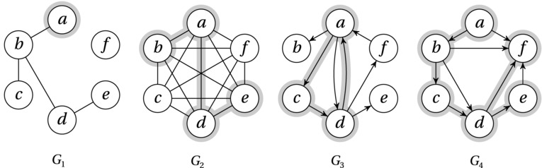
Figure C-1. Various types of graphs and digraphs

The basic graph definition gives us what is often called an undirected graph, which has a close relative: the directed graph, or digraph. The only difference is that the edges are no longer unordered pairs but ordered: An edge between nodes u and v is now either an edge (u,v) from u to v or an edge (v,u) from v to u. In other words, in a digraph G, E(G) is a relation over V(G). The graphs G₃ and G₄ in Figure C-1 are digraphs where the edge directions are indicated by arrowheads. Note that G₃ has what is called antiparallel edges between a and d, that is, edges going both ways. This is OK because (a,d) and (d,a) are different. Parallel edges, though (that is, the same edge, repeated) are not allowed—neither in graphs nor digraphs. (This follows from the fact that the edges form a set.) Note also that an undirected graph cannot have an edge between a node and itself, and even though this is possible in a digraph (so-called self-loops), the convention is to disallow it.

Note There are other relatives of the humble graph that do permit such things as parallel edges and self-loops. If we construct our network structure so that we can have multiple edges (that is, the edges now form a multiset ), and self-loops, we call it a (possibly directed) pseudograph. A pseudograph without self-loops is simply a multigraph. There are also more exotic versions, such as the hypergraph, where each edge can have multiple nodes.

Even though graphs and digraphs are quite different beasts, many of the principles and algorithms we deal with work just as well on either kind. Therefore, it is common to sometimes use the term graph in a more general sense, covering both directed and undirected graphs. Note also that in many contexts (such as when traversing or “moving around in” a graph), an undirected graph can be simulated by a directed one, by replacing each undirected edge with a pair of antiparallel directed edges. This is often done when actually implementing graphs as data structures (discussed in more detail in Chapter 2). If it is clear whether an edge is directed or undirected or if it doesn’t matter much, I’ll sometimes write uv instead of {u,v} or (u,v).

An edge is incident on its two nodes, called its end nodes. That is, uv is incident on u and v. If the edge is directed, we say that it leaves (or is incident from) u and that it enters (or is incident to) v. We call u and v its tail and head, respectively. If there is an edge uv in an undirected graph, the nodes u and v are adjacent and are called neighbors. The set of neighbors of a node v, also known as the neighborhood of v, is sometimes written as N(v). For example, the neighborhood N(b) of b in G₁ is {a,c,d}. If all nodes are pairwise adjacent, the graph is called complete (see G₂ in Figure C-1). For a directed graph, the edge uv means that v is adjacent to u, but the converse is true only if we also have an antiparallel edge vu. (In other words, the nodes adjacent to u are those we can “reach” from u by following the edges incident from it in the right direction.)

The number of (undirected) edges incident on a node v (that is, the size of N(v)) is called its degree, often written d(v). For example, in G₁ (Figure C-1), the node b has a degree of 3, while f has a degree of 0. (Zero-degree nodes are called isolated.) For directed graphs we can split this number into the in-degree (the number of incoming edges) and out-degree (the number of outgoing edges). We can also partition the neighborhood of a node into an in-neighborhood, sometimes called parents, and an out-neighborhood, or children.

One graph can be part of another. We say that a graph H = (W,F) is a subgraph of G = (V, E) or, conversely, that G is a supergraph of H, if W is a subset of V and F is a subset of E. That is, we can get H from G by (maybe) removing some nodes and edges. In Figure C-1, the highlighted nodes and edges indicate some example subgraphs that will be discussed in more detail in the following. If H is a subgraph of G, we often say that G contains H. We say that H spans G if W = V. That is, a spanning subgraph is one that covers all the nodes of the original graph (such as the one in graph G₄ in Figure C-1).

Paths are a special kind of graphs that are primarily of interest when they occur as subgraphs. A path is often identified by an sequence of (distinct) nodes, such as v₁, v₂, … , v_n, with edges (only) between pairs of successive nodes: E = {v₁v₂, v₂v₃, … , v_n–1v_n}. Note that in a directed graph, a path has to follow the directions of the edges; that is, all the edges in a path point forward. The length of a path is simply its edge count. We say that this is a path between v₁ to v_n (or, in the directed case, from v₁ to v_n). In the sample graph G₂, the highlighted subgraph is a path between b and e, for example, of length 3. If a path P₁ is a subgraph of another path P₂, we say that P₁ is a subpath of P₂. For example, the paths b, a, d and a, d, e in G₂ are both subpaths of b, a, d, e.

A close relative of the path is the cycle. A cycle is constructed by connecting the last node of a path to the first, as illustrated by the (directed) cycle through a, b, and c in G₃ (Figure C-1). The length of a cycle is also the number of edges it contains. Just like paths, cycles must follow the directions of the edges.

Note These definitions do not allow paths to cross themselves, that is, to contain cycles as subgraphs. A more general path-like notion, often called a walk, is simply an alternating sequence of nodes and edges (that is, not a graph in itself), which would allow nodes and edges to be visited multiple times and, in particular, would permit us to “walk in cycles.” The equivalent to a cycle is a closed walk, which starts and ends on the same node. To distinguish a path without cycles from a general walk, the term simple path is sometimes used.

A common generalization of the concepts discussed so far is the introduction of edge weights (or costs or lengths). Each edge e = uv is assigned a real number, w(e), sometimes written w(u,v), usually representing some form of cost associated with the edge. For example, if the nodes are geographic locations, the weights may represent driving distances in a road network. The weight w(G) of a graph G is simply the sum of w(e) for all edges e in G. We can then generalize the concept of path and cycle length to w(P) and w(C) for a path P and cycle C, respectively. The original definitions correspond to the case where each edge has a weight of 1. The distance between two nodes is the length of the shortest path between them. (Finding such shortest paths is dealt with extensively in the book, primarily in Chapter 9.)

A graph is connected if it contains a path between every pair of nodes. We say that a digraph is connected if the so-called underlying undirected graph (that is, the graph that results if we ignore edge directions) is connected. In Figure C-1, the only graph that is not connected is G₁. The maximal subgraphs of a graph that are connected are called its connected components. In Figure C-1, G₁ has two connected components, while the others have only one (each), because the graphs themselves are connected.

Note The term maximal, as it is used here, means that something cannot be extended and still have a given property. For example, a connected component is maximal in the sense that it is not a subgraph of a larger graph (one with more nodes or edges) that is also connected.

One family of graphs in particular is given a lot of attention, in computer science and elsewhere: graphs that do not contain cycles, or acyclic graphs. Acyclic graphs come in both directed and undirected variants, and these two versions have rather different properties. Let’s focus on the undirected kind first.

Another term for an undirected, acyclic graph is forest, and the connected components of a forest are called trees. In other words, a tree is a connected forest (that is, a forest consisting of a single connected component). For example, G₁ is a forest with two trees. In a tree, nodes with a degree of one are called leaves (or external nodes),⁴ while all others are called internal nodes. The larger tree in G₁, for example, has three leaves and two internal nodes. The smaller tree consists of only an internal node, although talking about leaves and internal nodes may not make much sense with fewer than three nodes.

Note Graphs with 0 or 1 nodes are called trivial and tend to make definitions trickier than necessary. In many cases, we simply ignore these cases, but sometimes it may be important to remember them. They can be quite useful as a starting point for induction, for example (covered in detail in Chapter 4).

Trees have several interesting and important properties, some of which are dealt with in relation to specific topics throughout the book. I’ll give you a few right here, though. Let T be an undirected graph with n nodes. Then the following statements are equivalent (Exercise 2-9 asks you to show that this is, indeed, the case):

T is a tree (that is, it is acyclic and connected).
T is acyclic and has n–1 edges.
T is connected and has n–1 edges.
Any two nodes are connected by exactly one path.
T is acyclic, but adding any new edge to it will create a cycle.
T is connected, but removing any edge yields two connected components.

In other words, any one of these statements of T, on its own, characterizes it as well as any of the others. If someone tells you that there is exactly one path between any pair of nodes in T, for example, you immediately know that it is connected and has n–1 edges and that it has no cycles.

Quite often, we anchor our tree by choosing a root node (or simply root). The result is called a rooted tree, as opposed to the free trees we’ve been looking at so far. (If it is clear from the context whether a tree has a root or not, I will simply use the unqualified term tree in both the rooted and free case.) Singling out a node like this lets us define the notions of up and down. Paradoxically, computer scientists (and graph theorists in general) tend to place the root at the top and the leaves at the bottom. (We probably should get out more …). For any node, up is in the direction of the root (along the single path between the node and the root). Down is then any other direction (automatically in the direction of the leaves). Note that in a rooted tree, the root is considered an internal node, not a leaf, even if it happens to have a degree of one.

Having properly oriented ourselves, we now define the depth of a node as its distance from the root, while its height is the length of longest downward path to any leaf. The height of the tree then is simply the height of the root. For example, consider the larger tree in G₁ in Figure C-1 and let a (highlighted) be the root. The height of the tree is then 3, while the depth of, say, c and d is 2. A level consists of all nodes that have the same depth. (In this case, level 0 consists of a, level 1 of b, level 2 of c and d, and level 3 of e.)

These directions also allow us to define other relationships, using rather intuitive terms from family trees (with the odd twist that we have only single parents). Your neighbor on the level above (that is, closer to the root) is your parent, while your neighbors on the level below are your children.⁵ (The root, of course, has no parent, and the leaves, no children.) More generally, any node you can reach by going upward is an ancestor, while any node you can reach by going down is a descendant. The tree spanning a node v and all its descendants is called the subtree rooted at v.

Note As opposed to subgraphs in general, the term subtree usually does not apply to all subgraphs that happen to be trees—especially not if we are talking about rooted trees.

Other similar terms generally have their obvious meanings. For example, siblings are nodes with a common parent. Sometimes siblings are ordered so that we can talk about the “first child” or “next sibling” of a node, for example. In this case, the tree is called an ordered tree.

As explained in Chapter 5, many algorithms are based on traversal, exploring graphs systematically, from some initial starting point (a start node). Although the way graphs are explored may differ, they have something in common. As long as they traverse the entire graph, they all give rise to spanning trees.⁶ (Spanning trees are simply spanning subgraphs that happen to be trees.) The spanning tree resulting from a traversal, called the traversal tree, is rooted at the starting node. The details of how this works will be revisited when dealing with the individual algorithms, but graph G₄ in Figure C-1 illustrates the concept. The highlighted subgraph is such a traversal tree, rooted at a. Note that all paths from a to the other nodes in the tree follow the edge directions; this is always the case for traversal trees in digraphs.

Note A digraph whose underlying graph is a rooted tree and where all the directed edges point away from the root (that is, all nodes can be reached by directed paths from the root) is called an arborescence, even though I’ll mostly talk about such graphs simply as trees. In other words, traversal in a digraph really gives you a traversal arborescence. The term oriented tree is used about both rooted (undirected) trees and arborescences because the edges of a rooted tree have an implicit direction away from the root.

Terminology fatigue setting in yet? Cheer up—only one graph concept left. As mentioned, directed graphs can be acyclic, just as undirected graphs can. The interesting thing is that these graphs don’t generally look much like forests of directed trees. Because the underlying undirected graph can be as cyclic as it wants, a directed acyclic graph, or DAG, can have an arbitrary structure (see Exercise 2-11), as long as the edges point in the right directions—that is, they are pointing so that no directed cycles exist. An example of this can be seen in sample graph G₄.

DAGs are quite natural as representations for dependencies because cyclic dependencies are generally impossible (or, at least, undesirable). For example, the nodes might be college courses, and an edge (u,v) would indicate that course u was a prerequisite for v. Sorting out such dependencies is the topic of the section on topological sorting in Chapter 5. DAGs also form the basis for the technique of dynamic programming, discussed in Chapter 8.

__________________

¹As quoted by Albert-László Barabási in his book Linked: TheNew Science of Networks (Basic Books, 2002).

²You probably didn’t even think of it as an issue, but you can assume that V and E don’t overlap.

³The functions would still be called V and E, even if we give the sets other names. For example, for a graph H = (W,F), we would have V(H) = W and E(H) = F.

⁴As explained later, though, the root is not considered a leaf. Also, for a graph consisting of only two connected nodes, calling them both leaves sometimes doesn’t make sense.

⁵Note that this is the same terminology as for the in- and out-neighborhoods in digraphs. The two concepts coincide once we start orienting the tree edges.

⁶This is true only if all nodes can be reached from the start node. Otherwise, the traversal may have to restart in several places, resulting in a spanning forest. Each component of the spanning forest will then have its own root.

Previous Chapter

Appendix B: List of Problems and Algorithms

Next Chapter

Appendix D: Hints for Exercises

Table of Contents for Python Algorithms: Mastering Basic Algorithms in the Python Language, Second Edition

Table of Contents for
Python Algorithms: Mastering Basic Algorithms in the Python Language, Second Edition