Table of Contents for
Python Algorithms: Mastering Basic Algorithms in the Python Language, Second Edition
 Python Algorithms: Mastering Basic Algorithms in the Python Language, Second Edition
Published by
Apress, 2015
Python Algorithms: Mastering Basic Algorithms in the Python Language, Second Edition
Published by
Apress, 2015
- Cover
- Title
- Copyright
- Dedication
- Contents at a Glance
- Contents
- About the Author
- About the Technical Reviewer
- Acknowledgments
- Preface
- Chapter 1: Introduction
- Chapter 2: The Basics
- Chapter 3: Counting 101
- Chapter 4: Induction and Recursion … and Reduction
- Chapter 5: Traversal: The Skeleton Key of Algorithmics
- Chapter 6: Divide, Combine, and Conquer
- Chapter 7: Greed Is Good? Prove It!
- Chapter 8: Tangled Dependencies and Memoization
- Chapter 9: From A to B with Edsger and Friends
- Chapter 10: Matchings, Cuts, and Flows
- Chapter 11: Hard Problems and (Limited) Sloppiness
- Appendix A: Pedal to the Metal: Accelerating Python
- Appendix B: List of Problems and Algorithms
- Appendix C: Graph Terminology
- Appendix D: Hints for Exercises
- Index

The Basics
Tracey: I didn’t know you were out there.
Zoe: Sort of the point. Stealth—you may have heard of it.
Tracey: I don’t think they covered that in basic.
— From “The Message,” episode 14 of Firefly
Before moving on to the mathematical techniques, algorithmic design principles, and classical algorithms that make up the bulk of this book, we need to go through some basic principles and techniques. When you start reading the following chapters, you should be clear on the meaning of phrases such as “directed, weighted graph without negative cycles” and “a running time of Θ(n lg n).” You should also have an idea of how to implement some fundamental structures in Python.
Luckily, these basic ideas aren’t at all hard to grasp. The main two topics of the chapter are asymptotic notation, which lets you focus on the essence of running times, and ways of representing trees and graphs in Python. There is also practical advice on timing your programs and avoiding some basic traps. First, though, let’s take a look at the abstract machines we algorists tend to use when describing the behavior of our algorithms.
Some Core Ideas in Computing
In the mid-1930s the English mathematician Alan Turing published a paper called “On computable numbers, with an application to the Entscheidungsproblem”1 and, in many ways, laid the groundwork for modern computer science. His abstract Turing machine has become a central concept in the theory of computation, in great part because it is intuitively easy to grasp. A Turing machine is a simple abstract device that can read from, write to, and move along an infinitely long strip of paper. The actual behavior of the machines varies. Each is a so-called finite state machine: It has a finite set of states (some of which indicate that it has finished), and every symbol it reads potentially triggers reading and/or writing and switching to a different state. You can think of this machinery as a set of rules. (“If I am in state 4 and see an X, I move one step to the left, write a Y, and switch to state 9.”) Although these machines may seem simple, they can, surprisingly enough, be used to implement any form of computation anyone has been able to dream up so far, and most computer scientists believe they encapsulate the very essence of what we think of as computing.
An algorithm is a procedure, consisting of a finite set of steps, possibly including loops and conditionals, that solves a given problem. A Turing machine is a formal description of exactly what problem an algorithm solves,2 and the formalism is often used when discussing which problems can be solved (either at all or in reasonable time, as discussed later in this chapter and in Chapter 11). For more fine-grained analysis of algorithmic efficiency, however, Turing machines are not usually the first choice. Instead of scrolling along a paper tape, we use a big chunk of memory that can be accessed directly. The resulting machine is commonly known as the random-access machine.
While the formalities of the random-access machine can get a bit complicated, we just need to know something about the limits of its capabilities so we don’t cheat in our algorithm analyses. The machine is an abstract, simplified version of a standard, single-processor computer, with the following properties:
- We don’t have access to any form of concurrent execution; the machine simply executes one instruction after the other.
- Standard, basic operations such as arithmetic, comparisons, and memory access all take constant (although possibly different) amounts of time. There are no more complicated basic operations such as sorting.
- One computer word (the size of a value that we can work with in constant time) is not unlimited but is big enough to address all the memory locations used to represent our problem, plus an extra percentage for our variables.
In some cases, we may need to be more specific, but this machine sketch should do for the moment.
We now have a bit of an intuition for what algorithms are, as well as the abstract hardware we’ll be running them on. The last piece of the puzzle is the notion of a problem. For our purposes, a problem is a relation between input and output. This is, in fact, much more precise than it might sound: A relation, in the mathematical sense, is a set of pairs—in our case, which outputs are acceptable for which inputs—and by specifying this relation, we’ve got our problem nailed down. For example, the problem of sorting may be specified as a relation between two sets, A and B, each consisting of sequences.3 Without describing how to perform the sorting (that would be the algorithm), we can specify which output sequences (elements of B) that would be acceptable, given an input sequence (an element of A). We would require that the result sequence consisted of the same elements as the input sequence and that the elements of the result sequence were in increasing order (each bigger than or equal to the previous). The elements of A here—that is, the inputs—are called problem instances; the relation itself is the actual problem.
To get our machine to work with a problem, we need to encode the input as zeros and ones. We won’t worry too much about the details here, but the idea is important, because the notion of running time complexity (as described in the next section) is based on knowing how big a problem instance is, and that size is simply the amount of memory needed to encode it. As you’ll see, the exact nature of this encoding usually won’t matter.
Asymptotic Notation
Remember the append versus insert example in Chapter 1? Somehow, adding items to the end of a list scaled better with the list size than inserting them at the front; see the nearby “Black Box” sidebar on list for an explanation. These built-in operations are both written in C, but assume for a minute that you reimplement list.append in pure Python; let’s say arbitrarily that the new version is 50 times slower than the original. Let’s also say you run your slow, pure-Python append-based version on a really slow machine, while the fast, optimized, insert-based version is run on a computer that is 1,000 times faster. Now the speed advantage of the insert version is a factor of 50,000. You compare the two implementations by inserting 100,000 numbers. What do you think happens?
Intuitively, it might seem obvious that the speedy solution should win, but its “speediness” is just a constant factor, and its running time grows faster than the “slower” one. For the example at hand, the Python-coded version running on the slower machine will, actually, finish in half the time of the other one. Let’s increase the problem size a bit, to 10 million numbers, for example. Now the Python version on the slow machine will be 2,000 times faster than the C version on the fast machine. That’s like the difference between running for about a minute and running almost a day and a half!
This distinction between constant factors (related to such things as general programming language performance and hardware speed, for example) and the growth of the running time, as problem sizes increase, is of vital importance in the study of algorithms. Our focus is on the big picture—the implementation-independent properties of a given way of solving a problem. We want to get rid of distracting details and get down to the core differences, but in order to do so, we need some formalism.
Python lists aren’t really lists in the traditional computer science sense of the word, and that explains the puzzle of why append is so much more efficient than insert. A classical list—a so-called linked list—is implemented as a series of nodes, each (except for the last) keeping a reference to the next. A simple implementation might look something like this:
class Node:
def __init__(self, value, next=None):
self.value = value
self.next = next
You construct a list by specifying all the nodes:
>>> L = Node("a", Node("b", Node("c", Node("d"))))
>>> L.next.next.value
'c'
This is a so-called singly linked list; each node in a doubly linked list would also keep a reference to the previous node.
The underlying implementation of Python’s list type is a bit different. Instead of several separate nodes referencing each other, a list is basically a single, contiguous slab of memory—what is usually known as an array. This leads to some important differences from linked lists. For example, while iterating over the contents of the list is equally efficient for both kinds (except for some overhead in the linked list), directly accessing an element at a given index is much more efficient in an array. This is because the position of the element can be calculated, and the right memory location can be accessed directly. In a linked list, however, one would have to traverse the list from the beginning.
The difference we’ve been bumping up against, though, has to do with insertion. In a linked list, once you know where you want to insert something, insertion is cheap; it takes roughly the same amount of time, no matter how many elements the list contains. That’s not the case with arrays: An insertion would have to move all elements that are to the right of the insertion point, possibly even moving all the elements to a larger array, if needed. A specific solution for appending is to use what’s often called a dynamic array, or vector.4 The idea is to allocate an array that is too big and then to reallocate it in linear time whenever it overflows. It might seem that this makes the append just as bad as the insert. In both cases, we risk having to move a large number of elements. The main difference is that it happens less often with the append. In fact, if we can ensure that we always move to an array that is bigger than the last by a fixed percentage (say 20 percent or even 100 percent), the average cost, amortized over many appends, is constant.
It’s Greek to Me!
Asymptotic notation has been in use (with some variations) since the late 19th century and is an essential tool in analyzing algorithms and data structures. The core idea is to represent the resource we’re analyzing (usually time but sometimes also memory) as a function, with the input size as its parameter. For example, we could have a program with a running time of T(n) = 2.4n + 7.
An important question arises immediately: What are the units here? It might seem trivial whether we measure the running time in seconds or milliseconds or whether we use bits or megabytes to represent problem size. The somewhat surprising answer, though, is that not only is it trivial, but it actually will not affect our results at all. We could measure time in Jovian years and problem size in kilograms (presumably the mass of the storage medium used), and it will not matter. This is because our original intention of ignoring implementation details carries over to these factors as well: The asymptotic notation ignores them all! (We do normally assume that the problem size is a positive integer, though.)
What we often end up doing is letting the running time be the number of times a certain basic operation is performed, while problem size is either the number of items handled (such as the number of integers to be sorted, for example) or, in some cases, the number of bits needed to encode the problem instance in some reasonable encoding.

Forgetting. Of course, the assert doesn’t work. (http://xkcd.com/379)
 Note Exactly how you encode your problems and solutions as bit patterns usually has little effect on the asymptotic running time, as long as you are reasonable. For example, avoid representing your numbers in the unary number system (1=1, 2=11, 3=111…).
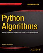
The asymptotic notation consists of a bunch of operators, written as Greek letters. The most important ones, and the only ones we’ll be using, are O (originally an omicron but now usually called “Big Oh”), Ω (omega), and Θ (theta). The definition for the O operator can be used as a foundation for the other two. The expression O(g), for some function g(n), represents a set of functions, and a function f(n) is in this set if it satisfies the following condition: There exists a natural number n0 and a positive constant c such that
f(n) ≤ cg(n)
for all n ≥ n0. In other words, if we’re allowed to tweak the constant c (for example, by running the algorithms on machines of different speeds), the function g will eventually (that is, at n0) grow bigger than f. See Figure 2-1 for an example.
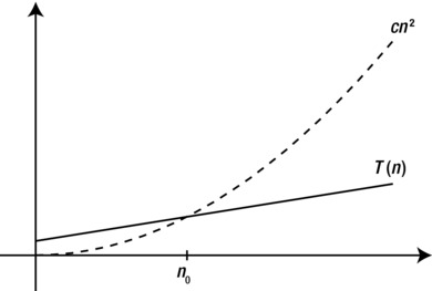
Figure 2-1. For values of n greater than n0, T(n) is less than cn2, so T(n) is O(n2)
This is a fairly straightforward and understandable definition, although it may seem a bit foreign at first. Basically, O(g) is the set of functions that do not grow faster than g. For example, the function n2 is in the set O(n2), or, in set notation, n2 ∈ O(n2). We often simply say that n2 is O(n2).
The fact that n2 does not grow faster than itself is not particularly interesting. More useful, perhaps, is the fact that neither 2.4n2 + 7 nor the linear function n does. That is, we have both
2.4n2 + 7 ∈ O(n2)
and
n ∈ O(n2).
The first example shows us that we are now able to represent a function without all its bells and whistles; we can drop the 2.4 and the 7 and simply express the function as O(n2), which gives us just the information we need. The second shows us that O can be used to express loose limits as well: Any function that is better (that is, doesn’t grow faster) than g can be found in O(g).
How does this relate to our original example? Well, the thing is, even though we can’t be sure of the details (after all, they depend on both the Python version and the hardware you’re using), we can describe the operations asymptotically: The running time of appending n numbers to a Python list is O(n), while inserting n numbers at its beginning is O(n2).
The other two, Ω and Θ, are just variations of O. Ω is its complete opposite: A function f is in Ω(g) if it satisfies the following condition: There exists a natural number n0 and a positive constant c such that
f(n) ≥ cg(n)
for all n ≥ n0. So, where O forms a so-called asymptotic upper bound, Ω forms an asymptotic lower bound.
Note Our first two asymptotic operators, O and Ω, are each other’s inverses: If f is O(g), then g is Ω(f). Exercise 2-3 asks you to show this.
The sets formed by Θ are simply intersections of the other two, that is, Θ(g) = O(g) ∩ Ω(g). In other words, a function f is in Θ(g) if it satisfies the following condition: There exists a natural number n0 and two positive constants c1 and c2 such that
c1g(n) ≤ f(n) ≤ c2g(n)
for all n ≥ n0. This means that f and g have the same asymptotic growth. For example, 3n2 + 2 is Θ(n2), but we could just as well write that n2 is Θ(3n2 + 2). By supplying an upper bound and a lower bound at the same time, the Θ operator is the most informative of the three, and I will use it when possible.
Rules of the Road
While the definitions of the asymptotic operators can be a bit tough to use directly, they actually lead to some of the simplest math ever. You can drop all multiplicative and additive constants, as well as all other “small parts” of your function, which simplifies things a lot.
As a first step in juggling these asymptotic expressions, let’s take a look at some typical asymptotic classes, or orders. Table 2-1 lists some of these, along with their names and some typical algorithms with these asymptotic running times, also sometimes called running-time complexities. (If your math is a little rusty, you could take a look at the sidebar “A Quick Math Refresher” later in the chapter.) An important feature of this table is that the complexities have been ordered so that each row dominates the previous one: If f is found higher in the table than g, then f is O(g).5
Table 2-1. Common Examples of Asymptotic Running Times
Complexity |
Name |
Examples, Comments |
|---|---|---|
Θ(1) |
Constant |
Hash table lookup and modification (see “Black Box” sidebar on dict). |
Θ(lg n) |
Logarithmic |
|
Θ(n) |
Linear |
Iterating over a list. |
Θ(n lg n) |
Loglinear |
Optimal sorting of arbitrary values (see Chapter 6). Same as Θ(lg n!). |
Θ(n2) |
Quadratic |
Comparing n objects to each other (see Chapter 3). |
Θ(n3) |
Cubic |
Floyd and Warshall’s algorithms (see Chapters 8 and 9). |
O(nk) |
Polynomial |
k nested for loops over n (if k is a positive integer). For any constant k > 0. |
Ω(kn) |
Exponential |
Producing every subset of n items (k = 2; see Chapter 3). Any k > 1. |
Θ(n!) |
Factorial |
Producing every ordering of n values. |
Note Actually, the relationship is even stricter: f is o(g), where the “Little Oh” is a stricter version if “Big Oh.” Intuitively, instead of “doesn’t grow faster than,” it means “grows slower than.” Formally, it states that f(n)/g(n) converges to zero as n grows to infinity. You don’t really need to worry about this, though.
Any polynomial (that is, with any power k > 0, even a fractional one) dominates any logarithm (that is, with any base), and any exponential (with any base k > 1) dominates any polynomial (see Exercises 2-5 and 2-6). Actually, all logarithms are asymptotically equivalent—they differ only by constant factors (see Exercise 2-4). Polynomials and exponentials, however, have different asymptotic growth depending on their exponents or bases, respectively. So, n5 grows faster than n4, and 5n grows faster than 4n.
The table primarily uses Θ notation, but the terms polynomial and exponential are a bit special, because of the role they play in separating tractable (“solvable”) problems from intractable (“unsolvable”) ones, as discussed in Chapter 11. Basically, an algorithm with a polynomial running time is considered feasible, while an exponential one is generally useless. Although this isn’t entirely true in practice, (Θ(n100) is no more practically useful than Θ(2n)); it is, in many cases, a useful distinction.6 Because of this division, any running time in O(nk), for any k > 0, is called polynomial, even though the limit may not be tight. For example, even though binary search (explained in the “Black Box” sidebar on bisect in Chapter 6) has a running time of Θ(lg n), it is still said to be a polynomial-time (or just polynomial) algorithm. Conversely, any running time in Ω(kn)—even one that is, say, Θ(n!)—is said to be exponential.
Now that we have an overview of some important orders of growth, we can formulate two simple rules:
- In a sum, only the dominating summand matters.
For example, Θ(n2 + n3 + 42) = Θ(n3).
- In a product, constant factors don’t matter.
For example, Θ(4.2n lg n) = Θ(n lg n).
In general, we try to keep the asymptotic expressions as simple as possible, eliminating as many unnecessary parts as we can. For O and Ω, there is a third principle we usually follow:
- Keep your upper or lower limits tight.
In other words, we try to make the upper limits low and the lower limits high. For example, although n2 might technically be O(n3), we usually prefer the tighter limit, O(n2). In most cases, though, the best thing is to simply use Θ.
A practice that can make asymptotic expressions even more useful is that of using them instead of actual values, in arithmetic expressions. Although this is technically incorrect (each asymptotic expression yields a set of functions, after all), it is quite common. For example, Θ(n2) + Θ(n3) simply means f + g, for some (unknown) functions f and g, where f is Θ(n2) and g is Θ(n3). Even though we cannot find the exact sum f + g, because we don’t know the exact functions, we can find the asymptotic expression to cover it, as illustrated by the following two “bonus rules:”
- Θ(f) + Θ(g) = Θ(f + g)
- Θ(f) · Θ(g) = Θ(f · g)
Exercise 2-8 asks you to show that these are correct.
Taking the Asymptotics for a Spin
Let’s take a look at some simple programs and see whether we can determine their asymptotic running times. To begin with, let’s consider programs where the (asymptotic) running time varies only with the problem size, not the specifics of the instance in question. (The next section deals with what happens if the actual contents of the instances matter to the running time.) This means, for example, that if statements are rather irrelevant for now. What’s important is loops, in addition to straightforward code blocks. Function calls don’t really complicate things; just calculate the complexity for the call and insert it at the right place.
Note There is one situation where function calls can trip us up: when the function is recursive. This case is dealt with in Chapters 3 and 4.
The loop-free case is simple: we are executing one statement before another, so their complexities are added. Let’s say, for example, that we know that for a list of size n, a call to append is Θ(1), while a call to insert at position 0 is Θ(n). Consider the following little two-line program fragment, where nums is a list of size n:
nums.append(1)
nums.insert(0,2)
We know that the line first takes constant time. At the time we get to the second line, the list size has changed and is now n + 1. This means that the complexity of the second line is Θ(n + 1), which is the same as Θ(n). Thus, the total running time is the sum of the two complexities, Θ(1) + Θ(n) = Θ(n).
Now, let’s consider some simple loops. Here’s a plain for loop over a sequence with n elements (numbers, say; for example, seq = range(n)):8
s = 0
for x in seq:
    s += x
This is a straightforward implementation of what the sum function does: It iterates over seq and adds the elements to the starting value in s. This performs a single constant-time operation (s += x) for each of the n elements of seq, which means that its running time is linear, or Θ(n). Note that the constant-time initialization (s = 0) is dominated by the loop here.
The same logic applies to the “camouflaged” loops we find in list (or set or dict) comprehensions and generator expressions, for example. The following list comprehension also has a linear running-time complexity:
squares = [x**2 for x in seq]
Several built-in functions and methods also have “hidden” loops in them. This generally applies to any function or method that deals with every element of a container, such as sum or map, for example.
Things get a little bit (but not a lot) trickier when we start nesting loops. Let’s say we want to sum up all possible products of the elements in seq; here’s an example:
s = 0
for x in seq:
    for y in seq:
        s += x*y
One thing worth noting about this implementation is that each product will be added twice. If 42 and 333 are both in seq, for example, we’ll add both 42*333 and 333*42. That doesn’t really affect the running time; it’s just a constant factor.
What’s the running time now? The basic rule is easy: The complexities of code blocks executed one after the other are just added. The complexities of nested loops are multiplied. The reasoning is simple: For each round of the outer loop, the inner one is executed in full. In this case, that means “linear times linear,” which is quadratic. In other words, the running time is Θ(n·n) = Θ(n2). Actually, this multiplication rule means that for further levels of nesting, we will just increment the power (that is, the exponent). Three nested linear loops give us Θ(n3), four give us Θ(n4), and so forth.
The sequential and nested cases can be mixed, of course. Consider the following slight extension:
s = 0
for x in seq:
    for y in seq:
        s += x*y
    for z in seq:
        for w in seq:
            s += x-w
It may not be entirely clear what we’re computing here (I certainly have no idea), but we should still be able to find the running time, using our rules. The z-loop is run for a linear number of iterations, and it contains a linear loop, so the total complexity there is quadratic, or Θ(n2). The y-loop is clearly Θ(n). This means that the code block inside the x-loop is Θ(n + n2). This entire block is executed for each round of the x-loop, which is run n times. We use our multiplication rule and get Θ(n(n + n2)) = Θ(n2 + n3) = Θ(n3), that is, cubic. We could arrive at this conclusion even more easily by noting that the y-loop is dominated by the z-loop and can be ignored, giving the inner block a quadratic running time. “Quadratic times linear” gives us cubic.
The loops need not all be repeated Θ(n) times, of course. Let’s say we have two sequences, seq1 and seq2, where seq1 contains n elements and seq2 contains m elements. The following code will then have a running time of Θ(nm).
s = 0
for x in seq1:
    for y in seq2:
        s += x*y
In fact, the inner loop need not even be executed the same number of times for each iteration of the outer loop. This is where things can get a bit fiddly. Instead of just multiplying two iteration counts, such as n and m in the previous example, we now have to sum the iteration counts of the inner loop. What that means should be clear in the following example:
seq1 = [[0, 1], [2], [3, 4, 5]]
s = 0
for seq2 in seq1:
    for x in seq2:
        s += x
The statement s += x is now performed 2 + 1 + 3 = 6 times. The length of seq2 gives us the running time of the inner loop, but because it varies, we cannot simply multiply it by the iteration count of the outer loop. A more realistic example is the following, which revisits our original example—multiplying every combination of elements from a sequence:
s = 0
n = len(seq)
for i in range(n-1):
    for j in range(i+1, n):
        s += seq[i] * seq[j]
To avoid multiplying objects with themselves or adding the same product twice, the outer loop now avoids the last item, and the inner loop iterates over the items only after the one currently considered by the outer one. This is actually a lot less confusing than it might seem, but finding the complexity here requires a little bit more care. This is one of the important cases of counting that is covered in the next chapter.9
Three Important Cases
Until now, we have assumed that the running time is completely deterministic and dependent only on input size, not on the actual contents of the input. That is not particularly realistic, however. For example, if you were to construct a sorting algorithm, you might start like this:
def sort_w_check(seq):
    n = len(seq)
    for i in range(n-1):
        if seq[i] > seq[i+1]:
            break
    else:
        return
    ...
A check is performed before getting into the actual sorting: If the sequence is already sorted, the function simply returns.
Note The optional else clause on a loop in Python is executed if the loop has not been ended prematurely by a break statement.
This means that no matter how inefficient our main sorting is, the running time will always be linear if the sequence is already sorted. No sorting algorithm can achieve linear running time in general, meaning that this “best-case scenario” is an anomaly—and all of a sudden, we can’t reliably predict the running time anymore. The solution to this quandary is to be more specific. Instead of talking about a problem in general, we can specify the input more narrowly, and we often talk about one of three important cases:
- The best case. This is the running time you get when the input is optimally suited to your algorithm. For example, if the input sequence to sort_w_check were sorted, we would get the best-case running time, which would be linear.
- The worst case. This is usually the most useful case—the worst possible running time. This is useful because we normally want to be able to give some guarantees about the efficiency of our algorithm, and this is the best guarantee we can give in general.
- The average case. This is a tricky one, and I’ll avoid it most of the time, but in some cases it can be useful. Simply put, it’s the expected value of the running time, for random input, with a given probability distribution.
In many of the algorithms we’ll be working with, these three cases have the same complexity. When they don’t, we’ll often be working with the worst case. Unless this is stated explicitly, however, no assumptions can be made about which case is being studied. In fact, we may not be restricting ourselves to a single kind of input at all. What if, for example, we wanted to describe the running time of sort_w_check in general? This is still possible, but we can’t be quite as precise.
Let’s say the main sorting algorithm we’re using after the check is loglinear; that is, it has a running time of Θ(n lg n)). This is typical and, in fact, optimal in the general case for sorting algorithms. The best-case running time of our algorithm is then Θ(n), when the check uncovers a sorted sequence, and the worst-case running time is Θ(n lg n). If we want to give a description of the running time in general, however—for any kind of input—we cannot use the Θ notation at all. There is no single function describing the running time; different types of inputs have different running time functions, and these have different asymptotic complexity, meaning we can’t sum them up in a single Θ expression.
The solution? Instead of the “twin bounds” of Θ, we supply only an upper or lower limit, using O or Ω. We can, for example, say that sort_w_check has a running time of O(n lg n). This covers both the best and worst cases. Similarly, we could say it has a running time of Ω(n). Note that these limits are as tight as we can make them.
Note It is perfectly acceptable to use either of our asymptotic operators to describe either of the three cases discussed here. We could very well say that the worst-case running time of sort_w_check is Ω(n lg n), for example, or that the best case is O(n).
Empirical Evaluation of Algorithms
The main focus of this book is algorithm design and its close relative, algorithm analysis. There is, however, another important discipline of algorithmics that can be of vital importance when building real-world systems, and that is algorithm engineering, the art of efficiently implementing algorithms. In a way, algorithm design can be seen as a way of achieving low asymptotic running time by designing efficient algorithms, while algorithm engineering is focused on reducing the hidden constants in that asymptotic complexity.
Although I may offer some tips on algorithm engineering in Python here and there, it can be hard to predict exactly which tweaks and hacks will give you the best performance for the specific problems you’re working on—or, indeed, for your hardware or version of Python. These are exactly the kind of quirks asymptotics are designed to avoid. And in some cases, such tweaks and hacks may not be needed at all, because your program may be fast enough as it is. The most useful thing you can do in many cases is simply to try and see. If you have a tweak you think will improve your program, try it! Implement the tweak, and run some experiments. Is there an improvement? And if the tweak makes your code less readable and the improvement is small, is it really worth it?
Note This section is about evaluating your programs, not on the engineering itself. For some hints on speeding up Python programs, see Appendix A.
While there are theoretical aspects of so-called experimental algorithmics—that is, experimentally evaluating algorithms and their implementations—that are beyond the scope of this book, I’ll give you some practical starting tips that should get you pretty far.
Tip 1 If possible, don’t worry about it.
Worrying about asymptotic complexity can be important. Sometimes, it’s the difference between a solution and what is, in practice, a nonsolution. Constant factors in the running time, however, are often not all that critical. Try a straightforward implementation of your algorithm first and see whether that’s good enough. Actually, you might even try a naïve algorithm first; to quote programming guru Ken Thompson, “When in doubt, use brute force.” Brute force, in algorithmics, generally refers to a straightforward approach that just tries every possible solution, running time be damned! If it works, it works.
Tip 2 For timing things, use timeit.
The timeit module is designed to perform relatively reliable timings. Although getting truly trustworthy results, such as those you’d publish in a scientific paper, is a lot of work, timeit can help you get “good enough in practice” timings easily. Here’s an example:
>>> import timeit
>>> timeit.timeit("x = 2 + 2")
0.034976959228515625
>>> timeit.timeit("x = sum(range(10))")
0.92387008666992188
The actual timing values you get will quite certainly not be exactly like mine. If you want to time a function (which could, for example, be a test function wrapping parts of your code), it may be even easier to use timeit from the shell command line, using the -m switch:
$ python -m timeit -s"import mymodule as m" "m.myfunction()"
There is one thing you should be careful about when using timeit. Avoid side effects that will affect repeated execution. The timeit function will run your code multiple times for increased precision, and if earlier executions affect later runs, you are probably in trouble. For example, if you time something like mylist.sort(), the list would get sorted only the first time. The other thousands of times the statement is run, the list will already be sorted, making your timings unrealistically low. The same caution would apply to anything involving generators or iterators that could be exhausted, for example. You can find more details on this module and how it works in the standard library documentation.10
Tip 3 To find bottlenecks, use a profiler.
It is a common practice to guess which part of your program needs optimization. Such guesses are quite often wrong. Instead of guessing wildly, let a profiler find out for you! Python comes with a few profiler variants, but the recommended one is cProfile. It’s as easy to use as timeit but gives more detailed information about where the execution time is spent. If your main function is main, you can use the profiler to run your program as follows:
import cProfile
cProfile.run('main()')
This should print out timing results about the various functions in your program. If the cProfile module isn’t available on your system, use profile instead. Again, more information is available in the library reference. If you’re not so interested in the details of your implementation but just want to empirically examine the behavior of your algorithm on a given problem instance, the trace module in the standard library can be useful—it can be used to count the number of times each statement is executed. You could even visualize the calls of your code using a tool such as Python Call Graph.11
Tip 4 Plot your results.
Visualization can be a great tool when figuring things out. Two common plots for looking at performance are graphs,12 for example of problem size versus running time, and box plots, showing the distribution of running times. See 1Figure 2-2 for examples of these. A great package for plotting things with Python is matplotlib (available from http://matplotlib.org).
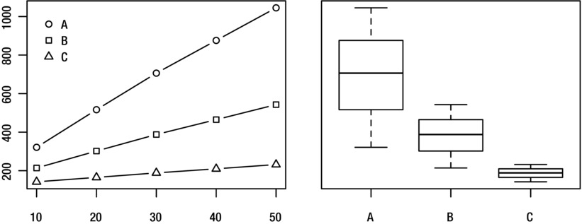
Figure 2-2. Visualizing running times for programs A, B, and C and problem sizes 10–50
Tip 5 Be careful when drawing conclusions based on timing comparisons.
This tip is a bit vague, but that’s because there are so many pitfalls when drawing conclusions about which way is better, based on timing experiments. First, any differences you observe may be because of random variations. If you’re using a tool such as timeit, this is less of a risk, because it repeats the statement to be timed many times (and even runs the whole experiment multiple times, keeping the best run). Still, there will be random variations, and if the difference between two implementations isn’t greater than what can be expected from this randomness, you can’t really conclude that they’re different. (You can’t conclude that they aren’t, either.)
Note If you need to draw a conclusion when it’s a close call, you can use the statistical technique of hypothesis testing. However, for practical purposes, if the difference is so small you’re not sure, it probably doesn’t matter which implementation you choose, so go with your favorite.
This problem is compounded if you’re comparing more than two implementations. The number of pairs to compare increases quadratically with the number of versions, as explained in Chapter 3, drastically increasing the chance that at least two of the versions will appear freakishly different, just by chance. (This is what’s called the problem of multiple comparisons.) There are statistical solutions to this problem, but the easiest practical way around it is to repeat the experiment with the two implementations in question. Maybe even a couple of times. Do they still look different?
Second, there are issues when comparing averages. At least, you should stick to comparing averages of actual timings. A common practice to get more meaningful numbers when performing timing experiments is to normalize the running time of each program, dividing it by the running time of some standard, simple algorithm. This can indeed be useful but can in some cases make your results less than meaningful. See the paper “How not to lie with statistics: The correct way to summarize benchmark results” by Fleming and Wallace for a few pointers. For some other perspectives, you could read Bast and Weber’s “Don’t compare averages,” or the more recent paper by Citron et al., “The harmonic or geometric mean: does it really matter?”
Third, your conclusions may not generalize. Similar experiments run on other problem instances or other hardware, for example, might yield different results. If others are to interpret or reproduce your experiments, it’s important that you thoroughly document how you performed them.
Tip 6 Be careful when drawing conclusions about asymptotics from experiments.
If you want to say something conclusively about the asymptotic behavior of an algorithm, you need to analyze it, as described earlier in this chapter. Experiments can give you hints, but they are by their nature finite, and asymptotics deal with what happens for arbitrarily large data sizes. On the other hand, unless you’re working in theoretical computer science, the purpose of asymptotic analysis is to say something about the behavior of the algorithm when implemented and run on actual problem instances, meaning that experiments should be relevant.
Suppose you suspect that an algorithm has a quadratic running time complexity, but you’re unable to conclusively prove it. Can you use experiments to support your claim? As explained, experiments (and algorithm engineering) deal mainly with constant factors, but there is a way. The main problem is that your hypothesis isn’t really testable through experiments. If you claim that the algorithm is, say, O(n2), no data can confirm or refute this. However, if you make your hypothesis more specific, it becomes testable. You might, for example, based on some preliminary results, believe that the running time will never exceed 0.24n2 + 0.1n + 0.03 seconds in your setup. Perhaps more realistically, your hypothesis might involve the number of times a given operation is performed, which you can test with the trace module. This is a testable—or, more specifically, refutable—hypothesis. If you run lots of experiments and you aren’t able to find any counter-examples, that supports your hypothesis to some extent. The neat thing is that, indirectly, you’re also supporting the claim that the algorithm is O(n2).
Implementing Graphs and Trees
The first example in Chapter 1, where we wanted to navigate Sweden and China, was typical of problems that can expressed in one of the most powerful frameworks in algorithmics—that of graphs. In many cases, if you can formulate what you’re working on as a graph problem, you’re at least halfway to a solution. And if your problem instances are in some form expressible as trees, you stand a good chance of having a really efficient solution.
Graphs can represent all kinds of structures and systems, from transportation networks to communication networks and from protein interactions in cell nuclei to human interactions online. You can increase their expressiveness by adding extra data such as weights or distances, making it possible to represent such diverse problems as playing chess or matching a set of people to as many jobs, with the best possible use of their abilities. Trees are just a special kind of graphs, so most algorithms and representations for graphs will work for them as well. However, because of their special properties (they are connected and have no cycles), some specialized and quite simple versions of both the representations and algorithms are possible. There are plenty of practical structures, such as XML documents or directory hierarchies, that can be represented as trees,13 so this “special case” is actually quite general.
If your memory of graph nomenclature is a bit rusty or if this is all new to you, take a look at Appendix C. Here are the highlights in a nutshell:
- A graph G = (V, E) consists of a set of nodes, V, and edges between them, E. If the edges have a direction, we say the graph is directed.
- Nodes with an edge between them are adjacent. The edge is then incident to both. The nodes that are adjacent to v are the neighbors of v. The degree of a node is the number of edges incident to it.
- A subgraph of G = (V, E) consists of a subset of V and a subset of E. A path in G is a subgraph where the edges connect the nodes in a sequence, without revisiting any node. A cycle is like a path, except that the last edge links the last node to the first.
- If we associate a weight with each edge in G, we say that G is a weighted graph. The length of a path or cycle is the sum of its edge weights, or, for unweighted graphs, simply the number of edges.
- A forest is a cycle-free graph, and a connected forest is a tree. In other words, a forest consists of one or more trees.
While phrasing your problem in graph terminology gets you far, if you want to implement a solution, you need to represent the graphs as data structures somehow. This, in fact, applies even if you just want to design an algorithm, because you must know what the running times of different operations on your graph representation will be. In some cases, the graph will already be present in your code or data, and no separate structure will be needed. For example, if you’re writing a web crawler, automatically collecting information about web sites by following links, the graph is the Web itself. If you have a Person class with a friends attribute, which is a list of other Person instances, then your object model itself is a graph on which you can run various graph algorithms. There are, however, specialized ways of implementing graphs.
In abstract terms, what we are generally looking for is a way of implementing the neighborhood function, N(v), so that N[v] is some form of container (or, in some cases, merely an iterable object) of the neighbors of v. Like so many other books on the subject, I will focus on the two most well-known representations, adjacency lists and adjacency matrices, because they are highly useful and general. For a discussion of alternatives, see the section “A Multitude of Representations” later in this chapter.
BLACK BOX: DICT AND SET
One technique covered in detail in most algorithm books, and usually taken for granted by Python programmers, is hashing. Hashing involves computing some often seemingly random integer value from an arbitrary object. This value can then be used, for example, as an index into an array (subject to some adjustments to make it fit the index range).
The standard hashing mechanism in Python is available through the hash function, which calls the __hash__ method of an object:
>>> hash(42)
42
>>> hash("Hello, world!")
-1886531940
This is the mechanism that is used in dictionaries, which are implemented using so-called hash tables. Sets are implemented using the same mechanism. The important thing is that the hash value can be constructed in essentially constant time. It’s constant with respect to the hash table size but linear as a function of the size of the object being hashed. If the array that is used behind the scenes is large enough, accessing it using a hash value is also Θ(1) in the average case. The worst-case behavior is Θ(n), unless we know the values beforehand and can write a custom hash function. Still, hashing is extremely efficient in practice.
What this means to us is that accessing elements of a dict or set can be assumed to take constant expected time, which makes them highly useful building blocks for more complex structures and algorithms.
Note that the hash function is specifically used for use in hash tables. For other uses of hashing, such as in cryptography, there is the standard library module hashlib.
Adjacency Lists and the Like
One of the most intuitive ways of implementing graphs is using adjacency lists. Basically, for each node, we can access a list (or set or other container or iterable) of its neighbors. Let’s take the simplest way of implementing this, assuming we have n nodes, numbered 0 . . . n–1.
Note Nodes can be any objects, of course, or have arbitrary labels or names. Using integers in the range 0 . . . n–1 can make many implementations easier, though, because the node numbers can easily be used as indices.
Each adjacency (or neighbor) list is then just a list of such numbers, and we can place the lists themselves into a main list of size n, indexable by the node numbers. Usually, the ordering of these lists is arbitrary, so we’re really talking about using lists to implement adjacency sets. The term list in this context is primarily historical. In Python we’re lucky enough to have a separate set type, which in many cases is a more natural choice.
For an example that will be used to illustrate the various graph representations, see Figure 2-3.
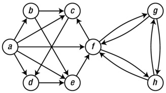
Figure 2-3. A sample graph used to illustrate various graph representations
Tip For tools to help you visualize your own graphs, see the sidebar “Graph Libraries” later in this chapter.
To begin with, assume that we have numbered the nodes, that is, a = 0, b = 1, and so forth. The graph can then be represented in a straightforward manner, as shown in Listing 2-1. Just as a convenience, I have assigned the node numbers to variables with the same names as the node labels in the figure. You can, of course, just work with the numbers directly. Which adjacency set belongs to which node is indicated by the comments. If you want, take a minute to confirm that the representation does, indeed, correspond to the figure.
Listing 2-1. A Straightforward Adjacency Set Representation
a, b, c, d, e, f, g, h = range(8)
N = [
    {b, c, d, e, f},    # a
    {c, e},             # b
    {d},                # c
    {e},                # d
    {f},                # e
    {c, g, h},          # f
    {f, h},             # g
    {f, g}              # h
]
Note In Python versions prior to 2.7 (or 3.0), you would write set literals as set([1, 2, 3]) rather than {1, 2, 3}. Note that an empty set is still written set() because {} is an empty dict.
The name N has been used here to correspond with the N function discussed earlier. In graph theory, N(v) represents the set of v’s neighbors. Similarly, in our code, N[v] is now a set of v’s neighbors. Assuming you have defined N as earlier in an interactive interpreter, you can now play around with the graph:
>>> b in N[a]  # Neighborhood membership
True
>>> len(N[f])  # Degree
3
Tip If you have some code in a source file, such as the graph definition in Listing 2-1, and you want to explore it interactively as in the previous example, you can run python with the -i switch, like this:
python -i listing_2_1.py
This will run the source file and start an interactive interpreter that continues where the source file left of, with any global definitions available for your experimentation.
Another possible representation, which can have a bit less overhead in some cases, is to replace the adjacency sets with actual adjacency lists. For an example of this, see Listing 2-2. The same operations are now available, except that membership checking is now Θ(n). This is a significant slowdown, but that is a problem only if you actually need it, of course. (If all your algorithm does is iterate over neighbors, using set objects would not only be pointless; the overhead would actually be detrimental to the constant factors of your implementation.)
Listing 2-2. Adjacency Lists
a, b, c, d, e, f, g, h = range(8)
N = [
    [b, c, d, e, f],    # a
    [c, e],             # b
    [d],                # c
    [e],                # d
    [f],                # e
    [c, g, h],          # f
    [f, h],             # g
    [f, g]              # h
]
It might be argued that this representation is really a collection of adjacency arrays, rather than adjacency lists in the classical sense, because Python’s list type is really a dynamic array behind the covers; see earlier “Black Box” sidebar about list. If you wanted, you could implement a linked list type and use that, rather than a Python list. That would allow you asymptotically cheaper inserts at arbitrary points in each list, but this is an operation you probably will not need, because you can just as easily append new neighbors at the end. The advantage of using list is that it is a well-tuned, fast data structure, as opposed to any list structure you could implement in pure Python.
A recurring theme when working with graphs is that the best representation depends on what you need to do with your graph. For example, using adjacency lists (or arrays) keeps the overhead low and lets you efficiently iterate over N(v) for any node v. However, checking whether u and v are neighbors is linear in the minimum of their degrees, which can be problematic if the graph is dense, that is, if it has many edges. In these cases, adjacency sets may be the way to go.
Tip We’ve also seen that deleting objects from the middle of a Python list is costly. Deleting from the end of a list takes constant time, though. If you don’t care about the order of the neighbors, you can delete arbitrary neighbors in constant time by overwriting them with the one that is currently last in the adjacency list, before calling the pop method.
A slight variation on this would be to represent the neighbor sets as sorted lists. If you aren’t modifying the lists much, you can keep them sorted and use bisection (see the “Black Box” sidebar on bisect in Chapter 6) to check for membership, which might lead to slightly less overhead in terms of memory use and iteration time but would lead to a membership check complexity of Θ(lg k), where k is the number of neighbors for the given node. (This is still very low. In practice, though, using the built-in set type is a lot less hassle.)
Yet another minor tweak on this idea is to use dicts instead of sets or lists. The neighbors would then be keys in this dict, and you’d be free to associate each neighbor (or out-edge) with some extra value, such as an edge weight. How this might look is shown in Listing 2-3, with arbitrary edge weights added.
Listing 2-3. Adjacency dicts with Edge Weights
a, b, c, d, e, f, g, h = range(8)
N = [
    {b:2, c:1, d:3, e:9, f:4},    # a
    {c:4, e:3},                   # b
    {d:8},                        # c
    {e:7},                        # d
    {f:5},                        # e
    {c:2, g:2, h:2},              # f
    {f:1, h:6},                   # g
    {f:9, g:8}                    # h
]
The adjacency dict version can be used just like the others, with the additional edge weight functionality:
>>> b in N[a]  # Neighborhood membership
True
>>> len(N[f])  # Degree
3
>>> N[a][b]    # Edge weight for (a, b)
2
If you want, you can use adjacency dicts even if you don’t have any useful edge weights or the like, of course (using, perhaps, None, or some other placeholder instead). This would give you the main advantages of the adjacency sets, but it would also work with very, very old versions of Python, which don’t have the set type.14
Until now, the main collection containing our adjacency structures—be they lists, sets, or dicts—has been a list, indexed by the node number. A more flexible approach, allowing us to use arbitrary, hashable, node labels, is to use a dict as this main structure.15 Listing 2-4 shows what a dict containing adjacency sets would look like. Note that nodes are now represented by characters.
Listing 2-4. A dict with Adjacency Sets
N = {
    'a': set('bcdef'),
    'b': set('ce'),
    'c': set('d'),
    'd': set('e'),
    'e': set('f'),
    'f': set('cgh'),
    'g': set('fh'),
    'h': set('fg')
}
Note If you drop the set constructor in Listing 2-4, you end up with adjacency strings, which would work as well, as immutable adjacency lists of characters, with slightly lower overhead. It’s a seemingly silly representation, but as I’ve said before, it depends on the rest of your program. Where are you getting the graph data from? Is it already in the form of text, for example? How are you going to use it?
Adjacency Matrices
The other common form of graph representation is the adjacency matrix. The main difference is the following: Instead of listing all neighbors for each node, we have a row (an array) with one position for each possible neighbor (that is, one for each node in the graph), and store a value, such as True or False, indicating whether that node is indeed a neighbor. Again, the simplest implementation is achieved using nested lists, as shown in Listing 2-5. Note that this, again, requires the nodes to be numbered from 0 to V–1. The truth values used are 1 and 0 (rather than True and False), simply to make the matrix more readable.
Listing 2-5. An Adjacency Matrix, Implemented with Nested Lists
a, b, c, d, e, f, g, h = range(8)

#     a b c d e f g h

N = [[0,1,1,1,1,1,0,0], # a
     [0,0,1,0,1,0,0,0], # b
     [0,0,0,1,0,0,0,0], # c
     [0,0,0,0,1,0,0,0], # d
     [0,0,0,0,0,1,0,0], # e
     [0,0,1,0,0,0,1,1], # f
     [0,0,0,0,0,1,0,1], # g
     [0,0,0,0,0,1,1,0]] # h
The way we’d use this is slightly different from the adjacency lists/sets. Instead of checking whether b is in N[a], you would check whether the matrix cell N[a][b] is true. Also, you can no longer use len(N[a]) to find the number of neighbors, because all rows are of equal length. Instead, use sum:
>>> N[a][b]    # Neighborhood membership
1
>>> sum(N[f])  # Degree
3
Adjacency matrices have some useful properties that are worth knowing about. First, as long as we aren’t allowing self-loops (that is, we’re not working with pseudographs), the diagonal is all false. Also, we often implement undirected graphs by adding edges in both directions to our representation. This means that the adjacency matrix for an undirected graph will be symmetric.
Extending adjacency matrices to allow for edge weights is trivial: Instead of storing truth values, simply store the weights. For an edge (u, v), let N[u][v] be the edge weight w(u, v) instead of True. Often, for practical reasons, we let nonexistent edges get an infinite weight. This is to guarantee that they will not be included in, say, shortest paths, as long as we can find a path along existent edges. It isn’t necessarily obvious how to represent infinity, but we do have some options.
One possibility is to use an illegal weight value, such as None, or -1 if all weights are known to be non-negative. Perhaps more useful in many cases is using a really large value. For integral weights, you could use sys.maxint, even though it’s not guaranteed to be the greatest possible value (long ints can be greater). There is, however, one value that is designed to represent infinity among floats: inf. It’s not available directly under that name in Python, but you can get it with the expression float('inf').16
Listing 2-6 shows what a weight matrix, implemented with nested lists, might look like. I’m using the same weights as I did in Listing 2-3, with inf = float('inf'). Note that the diagonal is still all zero, because even though we have no self-loops, weights are often interpreted as a form of distance, and the distance from a node to itself is customarily zero.
Listing 2-6. A Weight Matrix with Infinite Weight for Missing Edges
a, b, c, d, e, f, g, h = range(8)
inf = float('inf')

#       a    b    c    d    e    f    g    h

W = [[  0,   2,   1,   3,   9,   4, inf, inf], # a
     [inf,   0,   4, inf,   3, inf, inf, inf], # b
     [inf, inf,   0,   8, inf, inf, inf, inf], # c
     [inf, inf, inf,   0,   7, inf, inf, inf], # d
     [inf, inf, inf, inf,   0,   5, inf, inf], # e
     [inf, inf,   2, inf, inf,   0,   2,   2], # f
     [inf, inf, inf, inf, inf,   1,   0,   6], # g
     [inf, inf, inf, inf, inf,   9,   8,   0]] # h
Weight matrices make it easy to access edge weights, of course, but membership checking and finding the degree of a node, for example, or even iterating over neighbors must be done a bit differently now. You need to take the infinity value into account. Here’s an example:
>>> W[a][b] < inf   # Neighborhood membership
True
>>> W[c][e] < inf   # Neighborhood membership
False
>>> sum(1 for w in W[a] if w < inf) - 1  # Degree
5
Note that 1 is subtracted from the degree sum because we don’t want to count the diagonal. The degree calculation here is Θ(n), whereas both membership and degree could easily be found in constant time with the proper structure. Again, you should always keep in mind how you are going to use your graph and represent it accordingly.
SPECIAL-PURPOSE ARRAYS WITH NUMPY
The NumPy library has a lot of functionality related to multidimensional arrays. We don’t really need much of that for graph representation, but the NumPy array type is quite useful, for example, for implementing adjacency or weight matrices.
Where an empty list-based weight or adjacency matrix for n nodes is created, for example, like this
>>> N = [[0]*10 for i in range(10)]
in NumPy, you can use the zeros function:
>>> import numpy as np
>>> N = np.zeros([10,10])
The individual elements can then be accessed using comma-separated indices, as in A[u,v]. To access the neighbors of a given node, you use a single index, as in A[u].
If you have a relatively sparse graph, with only a small portion of the matrix filled in, you could save quite a bit of memory by using an even more specialized form of sparse matrix, available as part of the SciPy distribution, in the scipy.sparse module.
The NumPy package is available from http://www.numpy.org. You can get SciPy from http://www.scipy.org.
Note that you need to get a version of NumPy that will work with your Python version. If the most recent release of NumPy has not yet “caught up” with the Python version you want to use, you can compile and install directly from the source repository.
You can find more information about how to download, compile, and install NumPy, as well as detailed documentation on its use, on the web site.
Implementing Trees
Any general graph representation can certainly be used to represent trees because trees are simply a special kind of graph. However, trees play an important role on their own in algorithmics, and many special-purpose tree structures have been proposed. Most tree algorithms (even operations on search trees, discussed in Chapter 6) can be understood in terms of general graph ideas, but the specialized tree structures can make them easier to implement.
It is easiest to specialize the representation of rooted trees, where each edge is pointed downward, away from the root. Such trees often represent hierarchical partitionings of a data set, where the root represents all the objects (which are, perhaps, kept in the leaf nodes), while each internal node represents the objects found as leaves in the tree rooted at that node. You can even use this intuition directly, making each subtree a list containing its child subtrees. Consider the simple tree shown in Figure 2-4.
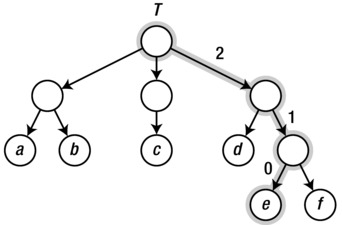
Figure 2-4. A sample tree with a highlighted path from the root to a leaf
We could represent that tree with lists of lists, like this:
>>> T = [["a", "b"], ["c"], ["d", ["e", "f"]]]
>>> T[0][1]
'b'
>>> T[2][1][0]
'e'
Each list is, in a way, a neighbor (or child) list of the anonymous internal nodes. In the second example, we access the third child of the root, the second child of that child, and finally the first child of that (path highlighted in the figure).
In some cases, we may know the maximum number of children allowed in any internal node. For example, a binary tree is one where each internal node has a maximum of two children. We can then use other representations, even objects with an attribute for each child, as shown in Listing 2-7.
Listing 2-7. A Binary Tree Class
class Tree:
    def __init__(self, left, right):
        self.left = left
        self.right = right
You can use the Tree class like this:
>>> t = Tree(Tree("a", "b"), Tree("c", "d"))
>>> t.right.left
'c'
You can, for example, use None to indicate missing children, such as when a node has only one child. You are, of course, free to combine techniques such as these to your heart’s content (for example, using a child list or child set in each node instance).
A common way of implementing trees, especially in languages that don’t have built-in lists, is the “first child, next sibling” representation. Here, each tree node has two “pointers,” or attributes referencing other nodes, just like in the binary tree case. However, the first of these refers to the first child of the node, while the second refers to its next sibling, as the name implies. In other words, each tree node refers to a linked list of siblings (its children), and each of these siblings refers to a linked list of its own. (See the “Black Box” sidebar on list, earlier in this chapter, for a brief introduction to linked lists.) Thus, a slight modification of the binary tree in Listing 2-7 gives us a multiway tree, as shown in Listing 2-8.
Listing 2-8. A Multiway Tree Class
class Tree:
    def __init__(self, kids, next=None):
        self.kids = self.val = kids
        self.next = next
The separate val attribute here is just to have a more descriptive name when supplying a value, such as 'c', instead of a child node. Feel free to adjust this as you want, of course. Here’s an example of how you can access this structure:
>>> t = Tree(Tree("a", Tree("b", Tree("c", Tree("d")))))
>>> t.kids.next.next.val
'c'
And here’s what that tree looks like:
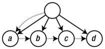
The kids and next attributes are drawn as dotted arrows, while the implicit edges of the trees are drawn solid. Note that I’ve cheated a bit and not drawn separate nodes for the strings "a", "b", and so on; instead, I’ve treated them as labels on their parent nodes. In a more sophisticated tree structure, you might have a separate value field in addition to kids, instead of using one attribute for both purposes.
Normally, you’d probably use more elaborate code (involving loops or recursion) to traverse the tree structure than the hard-coded path in this example. You’ll find more on that in Chapter 5. In Chapter 6, you’ll also see some discussion about multiway trees and tree balancing.
THE BUNCH PATTERN
When prototyping or even finalizing data structures such as trees, it can be useful to have a flexible class that will allow you to specify arbitrary attributes in the constructor. In these cases, the Bunch pattern (named by Alex Martelli in the Python Cookbook) can come in handy. There are many ways of implementing it, but the gist of it is the following:
class Bunch(dict):
def __init__(self, *args, **kwds):
super(Bunch, self).__init__(*args, **kwds)
self.__dict__ = self
There are several useful aspects to this pattern. First, it lets you create and set arbitrary attributes by supplying them as command-line arguments:
>>> x = Bunch(name="Jayne Cobb", position="Public Relations")
>>> x.name
'Jayne Cobb'
Second, by subclassing dict, you get lots of functionality for free, such as iterating over the keys/attributes or easily checking whether an attribute is present. Here’s an example:
>>> T = Bunch
>>> t = T(left=T(left="a", right="b"), right=T(left="c"))
>>> t.left
{'right': 'b', 'left': 'a'}
>>> t.left.right
'b'
>>> t['left']['right']
'b'
>>> "left" in t.right
True
>>> "right" in t.right
False
This pattern isn’t useful only when building trees, of course. You could use it for any situation where you’d want a flexible object whose attributes you could set in the constructor.
A Multitude of Representations
Even though there are a host of graph representations in use, most students of algorithms learn only the two types covered (with variations) so far in this chapter. Jeremy P. Spinrad writes, in his book Efficient Graph Representations, that most introductory texts are “particularly irritating” to him as a researcher in computer representations of graphs. Their formal definitions of the most well-known representations (adjacency matrices and adjacency lists) are mostly adequate, but the more general explanations are often faulty. He presents, based on misstatements from several texts, the following strawman’s17 comments on graph representations:
There are two methods for representing a graph in a computer: adjacency matrices and adjacency lists. It is faster to work with adjacency matrices, but they use more space than adjacency lists, so you will choose one or the other depending on which resource is more important to you.
These statements are problematic in several ways, as Spinrad points out. First, there are many interesting ways of representing graphs, not just the two listed here. For example, there are edge lists (or edge sets), which are simply lists containing all edges as node pairs (or even special edge objects); there are incidence matrices, indicating which edges are incident on which nodes (useful for multigraphs); and there are specialized methods for graph types such as trees (described earlier) and interval graphs (not discussed here). Take a look at Spinrad’s book for more representations than you will probably ever need. Second, the idea of space/time trade-off is quite misleading: There are problems that can be solved faster with adjacency lists than with adjacency arrays, and for random graphs, adjacency lists can actually use more space than adjacency matrices.
Rather than relying on simple, generalized statements such as the previous strawman’s comments, you should consider the specifics of your problem. The main criterion would probably be the asymptotic performance for what you’re doing. For example, looking up the edge (u, v) in an adjacency matrix is Θ(1), while iterating over u’s neighbors is Θ(n); in an adjacency list representation, both operations will be Θ(d(u)), that is, on the order of the number of neighbors the node has. If the asymptotic complexity of your algorithm is the same regardless of representation, you could perform some empirical tests, as discussed earlier in this chapter. Or, in many cases, you should simply choose the representation that makes your code clear and easily maintainable.
An important type of graph implementation not discussed so far is more of a nonrepresentation: Many problems have an inherent graphical structure—perhaps even a tree structure—and we can apply graph (or tree) algorithms to them without explicitly constructing a representation. In some cases, this happens when the representation is external to our program. For example, when parsing XML documents or traversing directories in the file system, the tree structures are just there, with existing APIs. In other cases, we are constructing the graph ourselves, but it is implicit. For example, if you want to find the most efficient solution to a given configuration of Rubik’s Cube, you could define a cube state, as well as operators for modifying that state. Even though you don’t explicitly instantiate and store all possible configurations, the possible states form an implicit graph (or node set), with the change operators as edges. You could then use an algorithm such as A* or Bidirectional Dijkstra (both discussed in Chapter 9) to find the shortest path to the solved state. In such cases, the neighborhood function N(v) would compute the neighbors on the fly, possibly returning them as a collection or some other form of iterable object.
The final kind of graph I’ll touch upon in this chapter is the subproblem graph. This is a rather deep concept that I’ll revisit several times, when discussing different algorithmic techniques. In short, most problems can be decomposed into subproblems: smaller problems that often have quite similar structure. These form the nodes of the subproblem graph, and the dependencies (that is, which subproblems depend on which) form the edges. Although we rarely apply graph algorithms directly to such subproblem graphs (they are more of a conceptual or mental tool), they do offer significant insights into such techniques as divide and conquer (Chapter 6) and dynamic programming (Chapter 8).
GRAPH LIBRARIES
The basic representation techniques described in this chapter will probably be enough for most of your graph algorithm coding, especially with some customization. However, there are some advanced operations and manipulations that can be tricky to implement, such as temporarily hiding or combining nodes, for example. There are third-party libraries out there that take care of some of these things, and several of them are even implemented as C extensions, potentially leading to a performance increase as a bonus. They can also be quite convenient to work with, and some of them have several graph algorithms available out of the box. While a quick web search will probably turn up the most actively supported graph libraries, here are a few to get you started:
- NetworkX: http://networkx.lanl.gov
- python-graph: http://code.google.com/p/python-graph
- Graphine: https://gitorious.org/graphine/pages/Home
- Graph-tool: http://graph-tool.skewed.de
There is also Pygr, a graph database (https://github.com/cjlee112/pygr); Gato, a graph animation toolbox (http://gato.sourceforge.net); and PADS, a collection of graph algorithms (http://www.ics.uci.edu/~eppstein/PADS).
While algorists generally work at a rather abstract level, actually implementing your algorithms takes some care. When programming, you’re bound to rely on components that you did not write yourself, and relying on such “black boxes” without any idea of their contents is a risky business. Throughout this book, you’ll find sidebars marked “Black Box,” briefly discussing various algorithms available as part of Python, either built into the language or found in the standard library. I’ve included these because I think they’re instructive; they tell you something about how Python works, and they give you glimpses of a few more basic algorithms.
However, these are not the only black boxes you’ll encounter. Not by a long shot. Both Python and the machinery it rests on use many mechanisms that can trip you up if you’re not careful. In general, the more important your program, the more you should mistrust such black boxes and seek to find out what’s going on under the covers. I’ll show you two traps to be aware of in the following sections, but if you take nothing else away from this section, remember the following:
- When performance is important, rely on actual profiling rather than intuition. You may have hidden bottlenecks, and they may be nowhere near where you suspect they are.
- When correctness is critical, the best thing you can do is calculate your answer more than once, using separate implementations, preferably written by separate programmers.
The latter principle of redundancy is used in many performance-critical systems and is also one of the key pieces of advice given by Foreman S. Acton in his book Real Computing Made Real, on preventing calculating errors in scientific and engineering software. Of course, in every scenario, you have to weigh the costs of correctness and performance against their value. For example, as I said before, if your program is fast enough, there’s no need to optimize it.
The following two sections deal with two rather different topics. The first is about hidden performance traps: operations that seem innocent enough but that can turn a linear operation into a quadratic one. The second is about a topic that is not often discussed in algorithm books, but it is important to be aware of, that is, the many traps of computing with floating-point numbers.
Hidden Squares
Consider the following two ways of looking for an element in a list:
>>> from random import randrange
>>> L = [randrange(10000) for i in range(1000)]
>>> 42 in L
False
>>> S = set(L)
>>> 42 in S
False
They’re both pretty fast, and it might seem pointless to create a set from the list—unnecessary work, right? Well, it depends. If you’re going to do many membership checks, it might pay off, because membership checks are linear for lists and constant for sets. What if, for example, you were to gradually add values to a collection and for each step check whether the value was already added? This is a situation you’ll encounter repeatedly throughout the book. Using a list would give you quadratic running time, whereas using a set would be linear. That’s a huge difference. The lesson is that it’s important to pick the right built-in data structure for the job.
The same holds for the example discussed earlier, about using a deque rather than inserting objects at the beginning of a list. But there are some examples that are less obvious that can cause just as many problems. Take, for example, the following “obvious” way of gradually building a string, from a source that provides us with the pieces:
>>> s = ""
>>> for chunk in string_producer():
...     s += chunk
It works, and because of some really clever optimizations in Python, it actually works pretty well, up to a certain size—but then the optimizations break down, and you run smack into quadratic growth. The problem is that (without the optimizations) you need to create a new string for every += operation, copying the contents of the previous one. You’ll see a detailed discussion of why this sort of thing is quadratic in the next chapter, but for now, just be aware that this is risky business. A better solution would be the following:
>>> chunks = []
>>> for chunk in string_producer():
...     chunks.append(chunk)
...
>>> s = ''.join(chunks)
You could even simplify this further like so:
>>> s = ''.join(string_producer())
This version is efficient for the same reason that the earlier append examples were. Appending allows you to overallocate with a percentage so that the available space grows exponentially, and the append cost is constant when averaged (amortized) over all the operations.
There are, however, quadratic running times that manage to hide even better than this. Consider the following solution, for example:
>>> s = sum(string_producer(), '')
Traceback (most recent call last):
   ...
TypeError: sum() can't sum strings [use ''.join(seq) instead]
Python complains and asks you to use ''.join() instead (and rightly so). But what if you’re using lists?
>>> lists = [[1, 2], [3, 4, 5], [6]]
>>> sum(lists, [])
[1, 2, 3, 4, 5, 6]
This works, and it even looks rather elegant, but it really isn’t. You see, under the covers, the sum function doesn’t know all too much about what you’re summing, and it has to do one addition after another. That way, you’re right back at the quadratic running time of the += example for strings. Here’s a better way:
>>> res = []
>>> for lst in lists:
...    res.extend(lst)
Just try timing both versions. As long as lists is pretty short, there won’t be much difference, but it shouldn’t take long before the sum version is thoroughly beaten.
The Trouble with Floats
Most real numbers have no exact finite representation. The marvelous invention of floating-point numbers makes it seem like they do, though, and even though they give us a lot of computing power, they can also trip us up. Big time. In the second volume of The Art of Computer Programming, Knuth says, “Floating point computation is by nature inexact, and programmers can easily misuse it so that the computed answers consist almost entirely of ‘noise.’”18
Python is pretty good at hiding these issues from you, which can be a good thing if you’re seeking reassurance, but it may not help you figure out what’s really going on. For example, in current version of Python, you’ll get the following reasonable behavior:
>>> 0.1
0.1
It certainly looks like the number 0.1 is represented exactly. Unless you know better, it would probably surprise you to learn that it’s not. Try an earlier version of Python (say, 2.6), where the black box was slightly more transparent:
>>> 0.1
0.10000000000000001
Now we’re getting somewhere. Let’s go a step further (feel free to use an up-to-date Python here):
>>> sum(0.1 for i in range(10)) == 1.0
False
Ouch! That’s not what you’d expect without previous knowledge of floats.
The thing is, integers can be represented exactly in any number system, be it binary, decimal, or something else. Real numbers, though, are a bit trickier. The official Python tutorial has an excellent section on this,19 and David Goldberg has written a great and thorough tutorial paper. The basic idea should be easy enough to grasp if you consider how you’d represent 1/3 as a decimal number. You can’t do it exactly, right? If you were using the ternary number system, though (base 3), it would be easily represented as 0.1.
The first lesson here is to never compare floats for equality. It generally doesn’t make sense. Still, in many applications such as computational geometry, you’d very much like to do just that. Instead, you should check whether they are approximately equal. For example, you could take the approach of assertAlmostEqual from the unittest module:
>>> def almost_equal(x, y, places=7):
...     return round(abs(x-y), places) == 0
...
>>> almost_equal(sum(0.1 for i in range(10)), 1.0)
True
There are also tools you can use if you need exact decimal floating-point numbers, for example the decimal module.
>>> from decimal import *
>>> sum(Decimal("0.1") for i in range(10)) == Decimal("1.0")
True
This module can be essential if you’re working with financial data, for example, where you need exact calculations with a certain number of decimals. In certain mathematical or scientific applications, you might find tools such as Sage useful:20
sage: 3/5 * 11/7 + sqrt(5239)
13*sqrt(31) + 33/35
As you can see, Sage does its math symbolically, so you get exact answers, although you can also get decimal approximations, if needed. This sort of symbolic math (or the decimal module) is nowhere near as efficient as using the built-in hardware capabilities for floating-point calculations, though.
If you find yourself doing floating-point calculations where accuracy is key (that is, you’re not just sorting them or the like), a good source of information is Acton’s book, mentioned earlier. Let’s just briefly look at an example of his: You can easily lose significant digits if you subtract two nearly equal subexpressions. To achieve higher accuracy, you’ll need to rewrite your expressions. Consider, for example, the expression sqrt(x+1)-sqrt(x), where we assume that x is very big. The thing to do would be to get rid of the risky subtraction. By multiplying and dividing by sqrt(x+1)+sqrt(x), we end up with an expression that is mathematically equivalent to the original but where we have eliminated the subtraction: 1.0/(sqrt(x+1)+sqrt(x)). Let’s compare the two versions:
>>> from math import sqrt
>>> x = 8762348761.13
>>> sqrt(x + 1) - sqrt(x)
5.341455107554793e-06
>>> 1.0/(sqrt(x + 1) + sqrt(x))
5.3414570026237696e-06
As you can see, even though the expressions are equivalent mathematically, they give different answers (with the latter being more accurate).
A QUICK MATH REFRESHER
If you’re not entirely comfortable with the formulas used in Table 2-1, here is a quick rundown of what they mean: A power, like x y (x to the power of y), is basically x times itself y times. More precisely, x occurs as a factor y times. Here, x is called the base, and y is the exponent (or sometimes the power). So, for example, 32 = 9. Nested powers simply have their exponents multiplied: (32)4 = 38. In Python, you write powers as x**y.
A polynomial is just a sum of several powers, each with its own constant factor. For example, 9x 5 + 2x 2 + x + 3.
You can have fractional powers, too, as a kind of inverse: (x y )1/y = x. These are sometimes called roots, such as the square root for the inverse of squaring. In Python you can get square roots either using the sqrt function from the math module or simply using x**0.5.
Roots are inverses in that they “undo” the effects of powers. Logarithms are another kind of inverse. Each logarithm has a fixed base; the most common one in algorithmics is the base-2 logarithm, written log2 or simply lg. (The base-10 logarithm is conventionally written simply log, while the so-called natural logarithm, with base e, is written ln). The logarithm gives us the exponent we need for the given base, so if n = 2k, then lg n = k. In Python, you can use the log function of the math module to get logarithms.
The factorial, or n!, is calculated as n × (n–1) × (n–2) … 1. It can be used, among other things, to calculate the number of possible orderings of n elements. There are n possibilities for the first position, and for each of those there are n–1 remaining for the second, and so forth.
If this is still about as clear as mud, don’t worry. You’ll encounter powers and logarithms repeatedly throughout the book, in rather concrete settings, where their meanings should be understandable.
Summary
This chapter started with some important foundational concepts, defining somewhat loosely the notions of algorithms, abstract computers, and problems. This was followed by the two main topics, asymptotic notation and graphs. Asymptotic notation is used to describe the growth of a function; it lets us ignore irrelevant additive and multiplicative constants and focus on the dominating part. This allows us evaluate the salient features of the running time of an algorithm in the abstract, without worrying about the specifics of a given implementation. The three Greek letters O, Ω, and Θ give us upper, lower, and combined asymptotic limits, and each can be used on either of the best-case, worst-case, or average-case behavior of an algorithm. As a supplement to this theoretical analysis, I gave you some brief guidelines for testing your program.
Graphs are abstract mathematical objects, used to represent all kinds of network structures. They consist of a set of nodes, connected by edges, and the edges can have properties such as direction and weight. Graph theory has an extensive vocabulary, and a lot of it is summed up in Appendix C. The second part of the chapter dealt with representing these structures in actual Python programs, primarily using variations of adjacency lists and adjacency matrices, implemented with various combinations of list, dict, and set.
Finally, there was a section about the dangers of black boxes. You should look around for potential traps—things you use without knowing how they work. For example, some rather straightforward uses of built-in Python functions can give you a quadratic running time rather than a linear one. Profiling your program can, perhaps, uncover such performance problems. There are traps related to accuracy as well. Careless use of floating-point numbers, for example, can give you inaccurate answers. If it’s critical to get an accurate answer, the best solution may be to calculate it with two separately implemented programs, comparing the results.
If You’re Curious …
If you want to know more about Turing machines and the basics of computation, you might like The Annotated Turing by Charles Petzold. It’s structured as an annotated version of Turing’s original paper, but most of the contents are Petzold’s explanations of the main concepts, with lots of examples. It’s a great introduction to the topic. For an fundamental textbook on computation, you could take a look at Elements of the Theory of Computation by Lewis and Papadimitriou. For an easy-to-read, wide-ranging popular introduction to the basic concepts of algorithmics, I recommend Algorithmic Adventures: From Knowledge to Magic by Juraj Hromkovič. For more specifics on asymptotic analysis, a solid textbook, such as one of those discussed in Chapter 1, would probably be a good idea. The book by Cormen et al. is considered a good reference work for this sort of thing. You can certainly also find a lot of good information online, such as in Wikipedia,21 but you should double-check the information before relying on it for anything important, of course. If you want some historical background, you could read Donald Knuth’s paper “Big Omicron and big Omega and big Theta,” from 1976.
For some specifics on the perils and practices of algorithmic experiments, there are several good papers, such as “Towards a discipline of experimental algorithmics,” “On comparing classifiers,” “Don’t compare averages,” “How not to lie with statistics,” “Presenting data from experiments in algorithmics,” “Visual presentation of data by means of box plots,” and “Using finite experiments to study asymptotic performance” (details in the “References” section). For visualizing data, take a look at Beginning Python Visualization by Shai Vaingast.
There are many textbooks on graph theory—some are rather technical and advanced (such as those by Bang-Jensen and Gutin, Bondy and Murty, or Diestel, for example), and some are quite readable, even for the novice mathematician (such as the one by West). There are even specialized books on, say, types of graphs (Brandstädt et al., 1999) or graph representations (Spinrad, 2003). If this is a topic that interests you, you shouldn’t have any trouble finding lots of material, either in books or online. For more on best practices when using floating-point numbers, take a look at Foreman S. Acton’s Real Computing Made Real: Preventing Errors in Scientific Engineering Calculations.
Exercises
2-1. When constructing a multidimensional array using Python lists, you need to use for loops (or something equivalent, such as list comprehension). Why would it be problematic to create a 10×10 array with the expression [[0]*10]*10?
2-2. Assume perhaps a bit unrealistically that allocating a block of memory takes constant time, as long as you leave it uninitialized (that is, it contains whatever arbitrary “junk” was left there the last time it was used). You want an array of n integers, and you want to keep track of whether each entry is unitialized or whether it contains a number you put there. This is a check you want to be able to do in constant time for any entry. How would you do this with only constant time for initialization? And how could you use this to initialize an empty adjacency array in constant time, thereby avoiding an otherwise obligatory quadratic minimum running time?
2-3. Show that O and Ω are inverses of one another; that is, if f is O(g), then g is Ω(f), and vice versa.
2-4. Logarithms can have different bases, but algorists don’t usually care. To see why, consider the equation logb n = (loga n)/(loga b). First, can you see why this is true? Second, why does this mean that we usually don’t worry about bases?
2-5. Show that any increasing exponential (Θ(kn) for k > 1) asymptotically dominates any polynomial (Θ(n j) for j > 0).
2-6. Show that any polynomial (that is, Θ(nk), for any constant k > 0) asymptotically dominates any logarithm (that is, Θ(lg n)). (Note that the polynomials here include, for example, the square root, for k = 0.5.)
2-7. Research or conjecture the asymptotic complexity of various operations on Python lists, such as indexing, item assignment, reversing, appending, and inserting (the latter two discussed in the “Black Box” sidebar on list). How would these be different in a linked list implementation? What about, for example, list.extend?
2-8. Show that the expressions Θ(f) + Θ(g) = Θ(f + g) and Θ(f) · Θ(g) = Θ(f · g) are correct. Also, try your hand at max(Θ(f), Θ(g)) = Θ(max(f, g)) = Θ(f + g).
2-9. In Appendix C, you’ll find a numbered list of statements about trees. Show that they are equivalent.
2-10. Let T be an arbitrary rooted tree with at least three nodes, where each internal node has exactly two children. If T has n leaves, how many internal nodes does it have?
2-11. Show that a directed acyclic graph (DAG) can have any underlying structure whatsoever. Put differently, any undirected graph can be the underlying graph for a DAG, or, given a graph, you can always orient its edges so that the resulting digraph is a DAG.
2-12. Consider the following graph representation: You use a dictionary and let each key be a pair (tuple) of two nodes, with the corresponding value set to the edge weight. For example W[u, v] = 42. What would be the advantages and disadvantages of this representation? Could you supplement it to mitigate the downsides?
References
Acton, F. S. (2005). Real Computing Made Real: Preventing Errors in Scientific and Engineering Calculations. Dover Publications, Inc.
Bang-Jensen, J. and Gutin, G. (2002). Digraphs: Theory, Algorithms and Applications. Springer.
Bast, H. and Weber, I. (2005). Don’t compare averages. In Nikoletseas, S. E., editor, WEA, volume 3503 of Lecture Notes in Computer Science, pages 67–76. Springer.
Bondy, J. A. and Murty, U. S. R. (2008). Graph Theory. Springer.
Brandstädt, A., Le, V. B., and Spinrad, J. P. (1999). Graph Classes: A Survey. SIAM Monographs on Discrete Mathematics and Applications. Society for Industrial and Applied Mathematics.
Citron, D., Hurani, A., and Gnadrey, A. (2006). The harmonic or geometric mean: Does it really matter? ACM SIGARCH Computer Architecture News, 34(4):18–25.
Diestel, R. (2005). Graph Theory, third edition. Springer.
Fleming, P. J. and Wallace, J. J. (1986). How not to lie with statistics: The correct way to summarize benchmark results. Commun. ACM, 29(3):218–221.
Goldberg, D. (1991). What every computer scientist should know about floating-point arithmetic. ACM Computing Surveys (CSUR), 23(1):5–48. http://docs.sun.com/source/806-3568/ncg_goldberg.html.
Hromkovič, J. (2009). Algorithmic Adventures: From Knowledge to Magic. Springer.
Knuth, D. E. (1976). Big Omicron and big Omega and big Theta. ACM SIGACT News, 8(2):18–24.
Lewis, H. R. and Papadimitriou, C. H. (1998). Elements of the Theory of Computation, second edition. Prentice Hall, Inc.
Martelli, A., Ravenscroft, A., and Ascher, D., editors (2005). Python Cookbook, second edition. O’Reilly & Associates, Inc.
Massart, D. L., Smeyers-Verbeke, J., Capron, X., and Schlesier, K. (2005). Visual presentation of data by means of box plots. LCGC Europe, 18:215–218.
McGeoch, C., Sanders, P., Fleischer, R., Cohen, P. R., and Precup, D. (2002). Using finite experiments to study asymptotic performance. Lecture Notes in Computer Science, 2547:94–126.
Moret, B. M. E. (2002). Towards a discipline of experimental algorithmics. In Data Structures, Near Neighbor Searches, and Methodology: Fifth and Sixth DIMACS Implementation Challenges, volume 59 of DIMACS: Series in Discrete Mathematics and Theoretical Computer Science, pages 197–214. Americal American Mathematical Society.
Petzold, C. (2008). The Annotated Turing: A Guided Tour Through Alan Turing’s Historic Paper on Computability and the Turing Machine. Wiley Publishing, Inc.
Salzberg, S. (1997). On comparing classifiers: Pitfalls to avoid and a recommended approach. Data Mining and Knowledge Discovery, 1(3):317–328.
Sanders, P. (2002). Presenting data from experiments in algorithmics. Lecture Notes in Computer Science, 2547:181–196.
Spinrad, J. P. (2003). Efficient Graph Representations. Fields Institute Monographs. American Mathematical Society.
Turing, A. M. (1937). On computable numbers, with an application to the Entscheidungsproblem. Proceedings of the London Mathematical Society, s2-42(1):230–265.
Vaingast, S. (2009). Beginning Python Visualization: Crafting Visual Transformation Scripts. Apress.
West, D. B. (2001). Introduction to Graph Theory, second edition. Prentice Hall, Inc.
___________________
1The Entscheidungsproblem is a problem posed by David Hilbert, which basically asks whether an algorithm exists that can decide, in general, whether a mathematical statement is true or false. Turing (and Alonzo Church before him) showed that such an algorithm cannot exist.
2There are also Turing machines that don’t solve any problems—machines that simply never stop. These still represent what we might call programs, but we usually don’t call them algorithms.
3Because input and output are of the same type, we could actually just specify a relation between A and A.
4For an “out-of-the-box” solution for inserting objects at the beginning of a sequence, see the black-box sidebar on deque in Chapter 5.
5For the “Cubic” and “Polynomial” row, this holds only when k ≥ 3.
6Interestingly, once a problem is shown to have a polynomial solution, an efficient polynomial solution can quite often be found as well.
7I’m using lg rather than log here, but either one is fine.
8If the elements are ints, the running time of each += is constant. However, Python also support big integers, or longs, which automatically appear when your integers get big enough. This means you can break the constant-time assumption by using really huge numbers. If you’re using floats, that won’t happen (but see the discussion of float problems near the end of the chapter).
9Spoiler: The complexity of this example is still Θ(n2).
10https://docs.python.org/library/timeit.html
11http://pycallgraph.slowchop.com
12No, not the network kind, which is discussed later in this chapter. The other kind—plots of some measurement for every value of some parameter.
13With IDREFs and symlinks, respectively, XML documents and directory hierarchies are actually general graphs.
14Sets were introduced in Python 2.3, in the form of the sets module. The built-in set type has been available since Python 2.4.
15This, a dictionary with adjacency lists, is what Guido van Rossum uses in his article “Python Patterns—Implementing Graphs,” which is found online at https://www.python.org/doc/essays/graphs/.
16This expression is guaranteed to work from Python 2.6 onward. In earlier versions, special floating-point values were platform-dependent, although float('inf') or float('Inf') should work on most platforms.
17That is, the comments are inadequate and are presented to demonstrate the problem with most explanations.
18This kind of trouble has led to disaster more than once (see, for example, www.ima.umn.edu/~arnold/455.f96/disasters.html).
19http://docs.python.org/tutorial/floatingpoint.html.
20Sage is a tool for mathematical computation in Python and is available from http://sagemath.org.