Table of Contents for
Python Algorithms: Mastering Basic Algorithms in the Python Language, Second Edition
 Python Algorithms: Mastering Basic Algorithms in the Python Language, Second Edition
Published by
Apress, 2015
Python Algorithms: Mastering Basic Algorithms in the Python Language, Second Edition
Published by
Apress, 2015
- Cover
- Title
- Copyright
- Dedication
- Contents at a Glance
- Contents
- About the Author
- About the Technical Reviewer
- Acknowledgments
- Preface
- Chapter 1: Introduction
- Chapter 2: The Basics
- Chapter 3: Counting 101
- Chapter 4: Induction and Recursion … and Reduction
- Chapter 5: Traversal: The Skeleton Key of Algorithmics
- Chapter 6: Divide, Combine, and Conquer
- Chapter 7: Greed Is Good? Prove It!
- Chapter 8: Tangled Dependencies and Memoization
- Chapter 9: From A to B with Edsger and Friends
- Chapter 10: Matchings, Cuts, and Flows
- Chapter 11: Hard Problems and (Limited) Sloppiness
- Appendix A: Pedal to the Metal: Accelerating Python
- Appendix B: List of Problems and Algorithms
- Appendix C: Graph Terminology
- Appendix D: Hints for Exercises
- Index

Counting 101
The greatest shortcoming of the human race is our inability to understand the exponential function.
— Dr. Albert A. Bartlett, World Population Balance
Board of Advisors
At one time, when the famous mathematician Carl Friedrich Gauss was in primary school, his teacher asked the pupils to add all the integers from 1 to 100 (or, at least, that’s the most common version of the story). No doubt, the teacher expected this to occupy his students for a while, but Gauss produced the result almost immediately. This might seem to require lightning-fast mental arithmetic, but the truth is, the actual calculation needed is quite simple; the trick is really understanding the problem.
After the previous chapter, you may have become a bit jaded about such things. “Obviously, the answer is Θ(1),” you say. Well, yes ... but let’s say we were to sum the integers from 1 to n? The following sections deal with some important problems like this, which will crop up again and again in the analysis of algorithms. The chapter may be a bit challenging at times, but the ideas presented are crucial and well worth the effort. They’ll make the rest of the book that much easier to understand. First, I’ll give you a brief explanation of the concept of sums and some basic ways of manipulating them. Then come the two major sections of the chapter: one on two fundamental sums (or combinatorial problems, depending on your perspective) and the other on so-called recurrence relations, which you’ll need to analyze recursive algorithms later. Between these two is a little section on subsets, combinations, and permutations.
 Tip There’s quite a bit of math in this chapter. If that’s not your thing, you might want to skim it for now and come back to it as needed while reading the rest of the book. (Several of the ideas in this chapter will probably make the rest of the book easier to understand, though.)
The Skinny on Sums
In Chapter 2, I explained that when two loops are nested and the complexity of the inner one varies from iteration to iteration of the outer one, you need to start summing. In fact, sums crop up all over the place in algorithmics, so you might as well get used to thinking about them. Let’s start with the basic notation.
More Greek
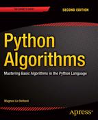
In Python, you might write the following:
x*sum(S) == sum(x*y for y in S)
With mathematical notation, you’d write this:
Can you see why this equation is true? This capital sigma can seem a bit intimidating if you haven’t worked with it before. It is, however, no scarier than the sum function in Python; the syntax is just a bit different. The sigma itself indicates that we’re doing a sum, and we place information about what to sum above, below, and to the right of it. What we place to the right (in the previous example, y and xy) are the values to sum, while we put a description of which items to iterate over below the sigma.
Instead of just iterating over objects in a set (or other collection), we can supply limits to the sum, like with range (except that both limits are inclusive). The general expression “sum f (i) for i = m to n” is written like this:

The Python equivalent would be as follows:
sum(f(i) for i in range(m, n+1))
It might be even easier for many programmers to think of these sums as a mathematical way of writing loops:
s = 0
for i in range(m, n+1):
    s += f(i)
The more compact mathematical notation has the advantage of giving us a better overview of what’s going on.
Working with Sums
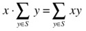
The sample equation in the previous section, where the factor x was moved inside the sum, is just one of several useful “manipulation rules” you’re allowed to use when working with sums. Here’s a summary of two of the most important ones (for our purposes):
Multiplicative constants can be moved in or out of sums. That’s also what the initial example in the previous section illustrated. This is the same rule of distributivity that you’ve seen in simpler sums many times: c(f (m) + ... + f (n)) = cf (m) + ... + cf (n).
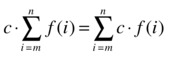
Instead of adding two sums, you can sum their added contents. This just means that if you’re going to sum up a bunch of stuff, it doesn’t matter how you do it; that is,
sum(f(i) for i in S) + sum(g(i) for i in S)
is exactly the same as sum(f(i) + g(i) for i in S).1 This is just an instance of associativity. If you want to subtract two sums, you can use the same trick. If you want, you can pretend you’re moving the constant factor –1 into the second sum.
A Tale of Two Tournaments
There are plenty of sums that you might find useful in your work, and a good mathematics reference will probably give you the solution to most of them. There are, however, two sums, or combinatorial problems, that cover the majority of the cases you’ll meet in this book—or, indeed, most basic algorithm work.
I’ve been explaining these two ideas repeatedly over the years, using many different examples and metaphors, but I think one rather memorable (and I hope understandable) way of presenting them is as two forms of tournaments.
Note There is, actually, a technical meaning of the word tournament in graph theory (a complete graph, where each edge is assigned a direction). That’s not what I’m talking about here, although the concepts are related.
There are many types of tournaments, but let’s consider two quite common ones, with rather catchy names. These are the round-robin tournament and the knockout tournament.
In a round-robin tournament (or, specifically, a single round-robin tournament), each contestant meets each of the others in turn. The question then becomes, how many matches or fixtures do we need, if we have, for example, n knights jousting? (Substitute your favorite competitive activity here, if you want.) In a knockout tournament, the competitors are arranged in pairs, and only the winner from each pair goes on to the next round. Here there are more questions to ask: For n knights, how many rounds do we need, and how many matches will there be, in total?
Shaking Hands
The round-robin tournament problem is exactly equivalent to another well-known puzzler: If you have n algorists meeting at a conference and they all shake hands, how many handshakes do you get? Or, equivalently, how many edges are there in a complete graph with n nodes (see Figure 3-1)? It’s the same count you get in any kind of “all against all” situations. For example, if you have n locations on a map and want to find the two that are closest to each other, the simple (brute-force) approach would be to compare all points with all others. To find the running time to this algorithm, you need to solve the round-robin problem. (A more efficient solution to this closest pair problem is presented in Chapter 6.)
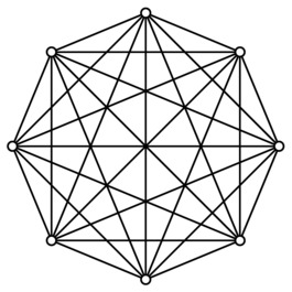
Figure 3-1. A complete graph, illustrating a round-robin tournament, or the handshake problem
You may very well have surmised that there will be a quadratic number of matches. “All against all” sounds an awful lot like “all times all,” or n2. Although it is true that the result is quadratic, the exact form of n2 isn’t entirely correct. Think about it—for one thing, only a knight with a death wish would ever joust against himself (or herself). And if Sir Galahad has crossed swords with Sir Lancelot, there is no need for Sir Lancelot to return the favor, because they surely have both fought each other, so a single match will do. A simple “n times n” solution ignores both of these factors, assuming that each knight gets a separate match against each of the knights (including themselves). The fix is simple: Let each knight get a match against all the others, yielding n(n–1), and then, because we now have counted each match twice (once for each participating knight), we divide by two, getting the final answer, n(n–1)/2, which is indeed Θ(n2).
Now we’ve counted these matches (or handshakes or map point comparisons) in one relatively straightforward way—and the answer may have seemed obvious. Well, what lies ahead may not exactly be rocket science either, but rest assured, there is a point to all of this . . . for now we count them all in a different way, which must yield the same result.
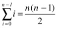
This other way of counting is this: The first knight jousts with n–1 others. Among the remaining, the second knight jousts with n–2. This continues down to the next to last, who fights the last match, against the last knight (who then fights zero matches against the zero remaining knights). This gives us the sum n–1 + n–2 + ... + 1 + 0, or sum(i for i in range(n)). We’ve counted each match only once, so the sum must yield the same count as before:
I could certainly just have given you that equation up front. I hope the extra packaging makes it slightly more meaningful to you. Feel free to come up with other ways of explaining this equation (or the others throughout this book), of course. For example, the insight often attributed to Gauss, in the story that opened this chapter, is that the sum of 1 through 100 can be calculated “from the outside,” pairing 1 with 100, 2 with 99, and so forth, yielding 50 pairs that all sum to 101. If you generalize this to the case of summing from 0 to n–1, you get the same formula as before. And can you see how all this relates to the lower-left half, below the diagonal, of an adjacency matrix?
Tip An arithmetic series is a sum where the difference between any two consecutive numbers is a constant. Assuming this constant is positive, the sum will always be quadratic. In fact, the sum of ik, where i = 1. . . n, for some positive constant k, will always be Θ(nk+1). The handshake sum is just a special case.
The Hare and the Tortoise
Let’s say our knights are 100 in number and that the tournament staff are still a bit tired from last year’s round robin. That’s quite understandable, as there would have been 4,950 matches. They decide to introduce the (more efficient) knockout system and want to know how many matches they’ll need. The solution can be a bit tricky to find ... or blindingly obvious, depending on how you look at it. Let’s look at it from the slightly tricky angle first. In the first round, all the knights are paired, so we have n/2 matches. Only half of them go on to the second round, so there we have n/4 matches. We keep on halving until the last match, giving us the sum n/2 + n/4 + n/8 + ... + 1, or, equivalently, 1 + 2 + 4 + ... + n/2. As you’ll see later, this sum has numerous applications, but what is the answer?
Now comes the blindingly obvious part: In each match, one knight is knocked out. All except the winner are knocked out (and they’re knocked out only once), so we need n–1 matches to leave only one man (or woman) standing. The tournament structure is illustrated as a rooted tree in Figure 3-2, where each leaf is a knight and each internal node represents a match. In other words:

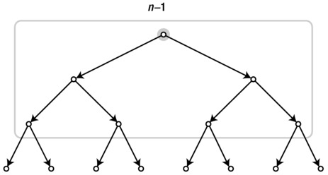
Figure 3-2. A perfectly balanced rooted, binary tree with n leaves and n–1 internal nodes (root highlighted). The tree may be undirected, but the edges can be thought of as implicitly pointing downward, as shown
The upper limit, h–1, is the number of rounds, or h the height of the binary tree, so 2h = n. Couched in this concrete setting, the result may not seem all that strange, but it sort of is, really. In a way, it forms the basis for the myth that there are more people alive than all those who have ever died. Even though the myth is wrong, it’s not that far-fetched! The growth of the human population is roughly exponential and currently doubles about every 50 years. Let’s say we had a fixed doubling time throughout history; this is not really true,2 but play along. Or, to simplify things even further, assume that each generation is twice as populous as the one before.3 Then, if the current generation consists of n individuals, the sum of all generations past will, as we have seen, be only n–1 (and, of course, some of them would still be alive).
WHY BINARY WORKS
We’ve just seen that when summing up the powers of two, you always get one less than the next power of two. For example, 1 + 2 + 4 = 8 – 1, or 1 + 2 + 4 + 8 = 16 – 1, and so forth. This is, from one perspective, exactly why binary counting works. A binary number is a string of zeros and ones, each of which determines whether a given power of two should be included in a sum (starting with 20 = 1 on the far right). So, for example, 11010 would be 2 + 8 + 16 = 26. Summing the first h of these powers would be equivalent to a number like 1111, with h ones. This is as far as we get with these h digits, but luckily, if these sum to n–1, the next power will be exactly n. For example, 1111 is 15, and 10000 is 16. (Exercise 3-3 asks you to show that this property lets you represent any positive integer as a binary number.)
Here’s the first lesson about doubling, then: A perfectly balanced binary tree (that is, a rooted tree where all internal nodes have two children and all leaves have the same depth) has n–1 internal nodes. There are, however, a couple more lessons in store for you on this subject. For example, I still haven’t touched upon the hare and tortoise hinted at in the section heading.
The hare and the tortoise are meant to represent the width and height of the tree, respectively. There are several problems with this image, so don’t take it too seriously, but the idea is that compared to each other (actually, as a function of each other), one grows very slowly, while the other grows extremely fast. I have already stated that n = 2h, but we might just as easily use the inverse, which follows from the definition of the binary logarithm: h = lg n; see Figure 3-3 for an illustration.
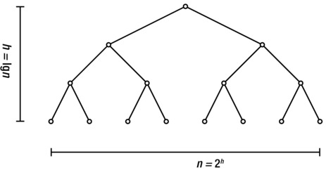
Figure 3-3. The height and width (number of leaves) of a perfectly balanced binary tree
Exactly how enormous the difference between these two is can be hard to fathom. One strategy would be to simply accept that they’re extremely different—meaning that logarithmic-time algorithms are super-sweet, while exponential-time algorithms are totally bogus—and then try to pick up examples of these differences wherever you can. Let me give you a couple of examples to get started. First let’s do a game I like to call “think of a particle.” I think of one of the particles in the visible universe, and you try to guess which one, using only yes/no questions. OK? Shoot!
This game might seem like sheer insanity, but I assure you, that has more to do with the practicalities (such that keeping track of which particles have been ruled out) than with the number of alternatives. To simplify these practicalities a bit, let’s do “think of a number” instead. There are many estimates for the number of particles we’re talking about, but 1090 (that is, a one followed by 90 zeros) would probably be quite generous. You can even play this game yourself, with Python:
>>> from random import randrange
>>> n = 10**90
>>> p = randrange(10**90)
You now have an unknown particle (particle number p) that you can investigate with yes/no questions (no peeking!). For example, a rather unproductive question might be as follows:
>>> p == 52561927548332435090282755894003484804019842420331
False
If you’ve ever played “twenty questions,” you’ve probably spotted the flaw here: I’m not getting enough “bang for the buck.” The best I can do with a yes/no question is halving the number of remaining options. So, for example:
>>> p < n/2
True
Now we’re getting somewhere! In fact, if you play your cards right (sorry for mixing metaphors—or, rather, games) and keep halving the remaining interval of candidates, you can actually find the answer in just under 300 questions. You can calculate this for yourself:
>>> from math import log
>>> log(n, 2) # base-two logarithm
298.97352853986263
If that seems mundane, let it sink in for a minute. By asking only yes/no questions, you can pinpoint any particle in the observable universe in about five minutes! This is a classic example of why logarithmic algorithms are so super-sweet. (Now try saying “logarithmic algorithm” ten times, fast.)
Note This is an example of bisection, or binary search, one of the most important and well-known logarithmic algorithms. It is discussed further in the “Black Box” sidebar on the bisect module in Chapter 6.
Let’s now turn to the bogus flip side of logarithms and ponder the equally weird exponentials. Any example for one is automatically an example for the other—if I asked you to start with a single particle and then double it repeatedly, you’d quickly fill up the observable universe. (It would take about 299 doublings, as we’ve seen.) This is just a slightly more extreme version of the old wheat and chessboard problem. If you place one grain of wheat on the first square of a chessboard, two on the second, four on the third, and so forth, how much wheat would you get?4 The number of grains in the last square would be 263 (we started at 20 = 1) and according to the sum illustrated in Figure 3-2, this means the total would be 264–1 = 18,446,744,073,709,551,615, or, for wheat, about 5 · 1014kg. That’s a lot of grain—hundreds of times the world’s total yearly production! Now imagine that instead of grain, we’re dealing with time. For a problem size n, your program uses 2n milliseconds. For n = 64, the program would then run for 584,542,046 years! To finish today, that program would have had to run since long before there were any vertebrates around to write the code. Exponential growth can be scary.
By now, I hope you’re starting to see how exponentials and logarithms are the inverses of one another. Before leaving this section, however, I’d like to touch upon another duality that arises when we’re dealing with our hare and tortoise: The number of doublings from 1 to n is, of course, the same as the number of halvings from n to 1. This is painfully obvious, but I’ll get back to it when we start working with recurrences in a bit, where this idea will be quite helpful. Take a look at Figure 3-4. The tree represents the doubling from 1 (the root node) to n (the n leaves), but I have also added some labels below the nodes, representing the halvings from n to 1. When working with recurrences, these magnitudes will represent portions of the problem instance, and the related amount of work performed, for a set of recursive calls. When we try to figure out the total amount of work, we’ll be using both the height of the tree and the amount of work performed at each level. We can see these values as a fixed number of tokens being passed down the tree. As the number of nodes doubles, the number of tokens per node is halved; the number of tokens per level remains n. (This is similar to the ice cream cones in the hint for Exercise 2-10.)
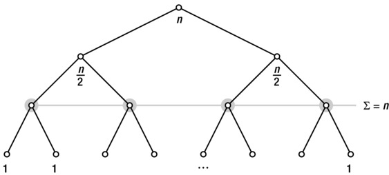
Figure 3-4. Passing n tokens down through the levels of a binary tree
Tip A geometric (or exponential ) series is a sum of ki, where i = 0...n, for some constant k. If k is greater than 1, the sum will always be Θ(k n+1). The doubling sum is just a special case.
Subsets, Permutations, and Combinations
The number of binary strings of length k should be easy to compute, if you’ve read the previous section. You can, for example, think of the strings as directions for walking from the root to leaves in a perfectly balanced binary tree. The string length, k, will be the height of the tree, and the number of possible strings will equal the number of leaves, 2k. Another, more direct way to see this is to consider the number of possibilities at each step: The first bit can be zero or one, and for each of these values, the second also has two possibilities, and so forth. It’s like k nested for loops, each running two iterations; the total count is still 2k.
PSEUDOPOLYNOMIALITY
Nice word, huh? It’s the name for certain algorithms with exponential running time that “look like” they have polynomial running times and that may even act like it in practice. The issue is that we can describe the running time as a function of many things, but we reserve the label “polynomial” for algorithms whose running time is a polynomial in the size of the input—the amount of storage required for a given instance, in some reasonable encoding. Let’s consider the problem of primality checking or answering the question “Is this number a prime?” This problem has a polynomial solution, but it’s not entirely obvious ... and the entirely obvious way to attack it actually yields a nonpolynomial solution.
Here’s my stab at a relatively direct solution:
def is_prime(n):
for i in range(2,n):
if n % i == 0: return False
return True
The algorithm here is to step through all positive integers smaller than n, starting at 2, checking whether they divide n. If one of them does, n is not a prime; otherwise, it is. This might seem like a polynomial algorithm, and indeed its running time is Θ(n). The problem is that n is not a legitimate problem size!
It can certainly be useful to describe the running time as linear in n, and we could even say that it is polynomial ... in n. But that does not give us the right to say that it is polynomial ... period. The size of a problem instance consisting of n is not n, but rather the number of bits needed to encode n, which, if n is a power of 2, is roughly lg n + 1. For an arbitrary positive integer, it’s actually floor(log(n,2))+1.
Let’s call this problem size (the number of bits) k. We then have roughly n = 2k–1. Our precious Θ(n) running time, when rewritten as a function of the actual problem size, becomes Θ(2k), which is clearly exponential.5 There are other algorithms like this, whose running times are polynomial only when interpreted as a function of a numeric value in the input. (One example is a solution to the knapsack problem, discussed in Chapter 8.) These are all called pseudopolynomial.
The relation to subsets is quite direct: If each bit represents the presence or absence of an object from a size-k set, each bit string represents one of the 2k possible subsets. Perhaps the most important consequence of this is that any algorithm that needs to check every subset of the input objects necessarily has an exponential running time complexity.
Although subsets are essential to know about for an algorist, permutations and combinations are perhaps a bit more marginal. You will probably run into them, though (and it wouldn’t be Counting 101 without them), so here is a quick rundown of how to count them.
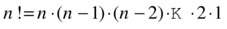
Permutations are orderings. If n people queue up for movie tickets, how many possible lines can we get? Each of these would be a permutation of the queuers. As mentioned in Chapter 2, the number of permutations of n items is the factorial of n, or n! (that includes the exclamation mark and is read “n factorial”). You can compute n! by multiplying n (the number of possible people in the first position) by n–1 (remaining options for the second position) and n–2 (third ...), and so forth, down to 1:
Not many algorithms have running times involving n! (although we’ll revisit this count when discussing limits to sorting, in Chapter 6). One silly example with an expected running time of Θ(n · n!) is the sorting algorithm bogosort, which consists of repeatedly shuffling the input sequence into a random order and checking whether the result is sorted.
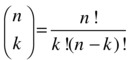
Combinations are a close relative of both permutations and subsets. A combination of k elements, drawn from a set of n, is sometimes written C(n, k), or, for those of a mathematical bent:

This is also called the binomial coefficient (or sometimes the choose function) and is read “n choose k.” While the intuition behind the factorial formula is rather straightforward, how to compute the binomial coefficient isn’t quite as obvious.6
Imagine (once again) you have n people lined up to see a movie, but there are only k places left in the theater. How many possible subsets of size k could possibly get in? That’s exactly C(n, k), of course, and the metaphor may do some work for us here. We already know that we have n! possible orderings of the entire line. What if we just count all these possibilities and let in the first k? The only problem then is that we’ve counted the subsets too many times. A certain group of k friends could stand at the head of the line in a lot of the permutations; in fact, we could allow these friends to stand in any of their k! possible permutations, and the remainder of the line could stand in any of their (n–k)! possible permutations without affecting who’s getting in. Aaaand this gives us the answer!
This formula just counts all possible permutations of the line (n!) and divides by the number of times we count each “winning subset,” as explained.
Note A different perspective on calculating the binomial coefficient will be given in Chapter 8, on dynamic programming.
Note that we’re selecting a subset of size k here, which means selection without replacement. If we just draw lots k times, we might draw the same person more than once, effectively “replacing” them in the pool of candidates. The number of possible results then would simply be nk. The fact that C(n, k) counts the number of possible subsets of size k and 2n counts the number of possible subsets in total gives us the following beautiful equation:

And that’s it for these combinatorial objects. It’s time for slightly more mind-bending prospect: solving equations that refer to themselves!
Tip For most math, the interactive Python interpreter is quite handy as a calculator; the math module contains many useful mathematical functions. For symbolic manipulation like we’ve been doing in this chapter, though, it’s not very helpful. There are symbolic math tools for Python, though, such as Sage (available from http://sagemath.org). If you just need a quick tool for solving a particularly nasty sum or recurrence (see the next section), you might want to check out Wolfram Alpha (http://wolframalpha.com). You just type in the sum or some other math problem, and out pops the answer.
Recursion and Recurrences
I’m going to assume that you have at least some experience with recursion, although I’ll give you a brief intro in this section and even more detail in Chapter 4. If it’s a completely foreign concept to you, it might be a good idea to look it up online or in some fundamental programming textbook.
The thing about recursion is that a function—directly or indirectly—calls itself. Here’s a simple example of how to recursively sum a sequence:
def S(seq, i=0):
    if i == len(seq): return 0
    return S(seq, i+1) + seq[i]
Understanding how this function works and figuring out its running time are two closely related tasks. The functionality is pretty straightforward: The parameter i indicates where the sum is to start. If it’s beyond the end of the sequence (the base case, which prevents infinite recursion), the function simply returns 0. Otherwise, it adds the value at position i to the sum of the remaining sequence. We have a constant amount of work in each execution of S, excluding the recursive call, and it’s executed once for each item in the sequence, so it’s pretty obvious that the running time is linear. Still, let’s look into it:
def T(seq, i=0):
    if i == len(seq): return 1
    return T(seq, i+1) + 1
This new T function has virtually the same structure as S, but the values it’s working with are different. Instead of returning a solution to a subproblem, like S does, it returns the cost of finding that solution. In this case, I’ve just counted the number of times the if statement is executed. In a more mathematical setting, you would count any relevant operations and use Θ(1) instead of 1, for example. Let’s take these two functions out for a spin:
>>> seq = range(1,101)
>>> s(seq)
5050
What do you know, Gauss was right! Let’s look at the running time:
>>> T(seq)
101
Looks about right. Here, the size n is 100, so this is n+1. It seems like this should hold in general:
>>> for n in range(100):
...     seq = range(n)
...     assert T(seq) == n+1
There are no errors, so the hypothesis does seem sort of plausible.
What we’re going to work on now is how to find nonrecursive versions of functions such as T, giving us definite running time complexities for recursive algorithms.
Doing It by Hand
To describe the running time of recursive algorithms mathematically, we use recursive equations, called recurrence relations. If our recursive algorithm is like S in the previous section, then the recurrence relation is defined somewhat like T. Because we’re working toward an asymptotic answer, we don’t care about the constant parts, and we implicitly assume that T(k) = Θ(1), for some constant k. That means we can ignore the base cases when setting up our equation (unless they don’t take a constant amount of time), and for S, our T can be defined as follows:
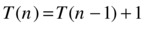
This means that the time it takes to compute S(seq, i), which is T (n), is equal to the time required for the recursive call S(seq, i+1), which is T (n–1), plus the time required for the access seq[i], which is constant, or Θ(1). Put another way, we can reduce the problem to a smaller version of itself, from size n to n–1, in constant time and then solve the smaller subproblem. The total time is the sum of these two operations.
Note As you can see, I use 1 rather than Θ(1) for the extra work (that is, time) outside the recursion. I could use the theta as well; as long as I describe the result asymptotically, it won’t matter much. In this case, using Θ(1) might be risky, because I’ll be building up a sum (1 + 1 + 1 ...), and it would be easy to mistakenly simplify this sum to a constant if it contained asymptotic notation (that is, Θ(1) + Θ(1) + Θ(1) ...).
Now, how do we solve an equation like this? The clue lies in our implementation of T as an executable function. Instead of having Python run it, we can simulate the recursion ourselves. The key to this whole approach is the following equation:
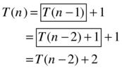
The two subformulas I’ve put in boxes are identical, which is sort of the point. My rationale for claiming that the two boxes are the same lies in our original recurrence, for if ...

... then:
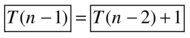
I’ve simply replaced n with n–1 in the original equation (of course, T((n–1)–1) = T (n–2)), and voilà, we see that the boxes are equal. What we’ve done here is to use the definition of T with a smaller parameter, which is, essentially, what happens when a recursive call is evaluated. So, expanding the recursive call from T (n–1), the first box, to T(n–2) + 1, the second box, is essentially simulating or “unraveling” one level of recursion. We still have the recursive call T (n–2) to contend with, but we can deal with that in the same way!
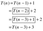
The fact that T(n–2) = T (n–3) + 1 (the two boxed expressions) again follows from the original recurrence relation. It’s at this point we should see a pattern: Each time we reduce the parameter by one, the sum of the work (or time) we’ve unraveled (outside the recursive call) goes up by one. If we unravel T (n) recursively i steps, we get the following:
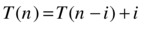
This is exactly the kind of expression we’re looking for—one where the level of recursion is expressed as a variable i. Because all these unraveled expressions are equal (we’ve had equations every step of the way), we’re free to set i to any value we want, as long as we don’t go past the base case (for example, T (1)), where the original recurrence relation is no longer valid. What we do is go right up to the base case and try to make T(n–i) into T (1), because we know, or implicitly assume, that T (1) is Θ(1), which would mean we had solved the entire thing. And we can easily do that by setting i = n–1:
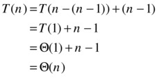
We have now, with perhaps more effort than was warranted, found that S has a linear running time, as we suspected. In the next section, I’ll show you how to use this method for a couple of recurrences that aren’t quite as straightforward.
Caution This method, called the method of repeated substitutions (or sometimes the iteration method ), is perfectly valid, if you’re careful. However, it’s quite easy to make an unwarranted assumption or two, especially in more complex recurrences. This means you should probably treat the result as a hypothesis and then check your answer using the techniques described in the section “Guessing and Checking” later in this chapter.
A Few Important Examples
The general form of the recurrences you’ll normally encounter is T (n) = a·T (g(n)) + f (n), where a represents the number of recursive calls, g(n) is the size of each subproblem to be solved recursively, and f (n) is any extra work done in the function, in addition to the recursive calls.
Tip It’s certainly possible to formulate recursive algorithms that don’t fit this schema, for example if the subproblem sizes are different. Such cases won’t be dealt with in this book, but some pointers for more information are given in the section “If You’re Curious ...,” near the end of this chapter.
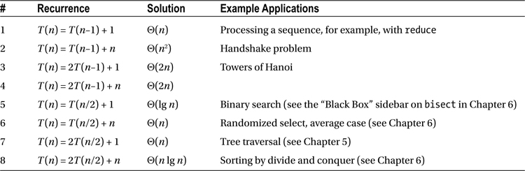
Table 3-1 summarizes some important recurrences—one or two recursive calls on problems of size n–1 or n/2, with either constant or linear additional work in each call. You’ve already seen recurrence number 1 in the previous section. In the following, I’ll show you how to solve the last four using repeated substitutions, leaving the remaining three (2 to 4) for Exercises 3-7 to 3-9.
Table 3-1. Some Basic Recurrences with Solutions, as Well as Some Sample Applications
Before we start working with the last four recurrences (which are all examples of divide and conquer recurrences, explained more in detail later in this chapter and in Chapter 6), you might want to refresh your memory with Figure 3-5. It summarizes the results I’ve discussed so far about binary trees; sneakily enough, I’ve already given you all the tools you need, as you’ll see in the following text.
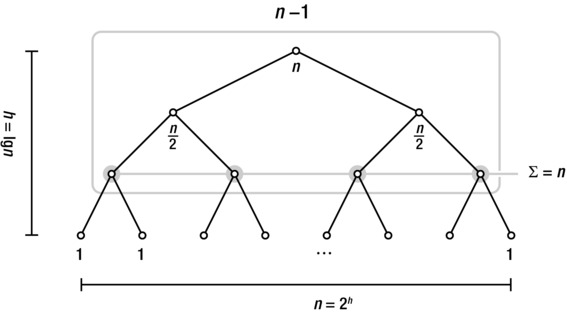
Figure 3-5. A summary of some important properties of perfectly balanced binary trees
Note I’ve already mentioned the assumption that the base case has constant time (T (k) = t0, k ≤ n0, for some constants t0 and n0). In recurrences where the argument to T is n/b, for some constant b, we run up against another technicality: The argument really should be an integer. We could achieve that by rounding (using floor and ceil all over the place), but it’s common to simply ignore this detail (really assuming that n is a power of b). To remedy the sloppiness, you should check your answers with the method described in “Guessing and Checking” later in this chapter.
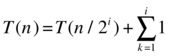
Look at recurrence 5. There’s only one recursive call, on half the problem, and a constant amount of work in addition. If we see the full recursion as a tree (a recursion tree), this extra work (f (n)) is performed in each node, while the structure of the recursive calls is represented by the edges. The total amount of work (T (n)) is the sum of f (n) over all the nodes (or those involved). In this case, the work in each node is constant, so we need to count only the number of nodes. Also, we have only one recursive call, so the full work is equivalent to a path from the root to a leaf. It should be obvious that T(n) is logarithmic, but let’s see how this looks if we try to unravel the recurrence, step-by-step:
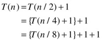
The curly braces enclose the part that is equivalent to the recursive call (T (...)) in the previous line. This stepwise unraveling (or repeated substitution) is just the first step of our solution method. The general approach is as follows:
- Unravel the recurrence until you see a pattern.
- Express the pattern (usually involving a sum), using a line number variable, i.
- Choose i so the recursion reaches its base case (and solve the sum).
The first step is what we have done already. Let’s have a go at step 2:
I hope you agree that this general form captures the pattern emerging from our unraveling: For each unraveling (each line further down), we halve the problem size (that is, double the divisor) and add another unit of work (another 1). The sum at the end is a bit silly. We know we have i ones, so the sum is clearly just i. I’ve written it as a sum to show the general pattern of the method here.
To get to the base case of the recursion, we must get T (n/2i) to become, say, T (1). That just means we have to halve our way from n to 1, which should be familiar by now: The recursion height is logarithmic, or i = lg n. Insert that into the pattern, and you get that T (n) is, indeed, Θ(lg n).
The unraveling for recurrence 6 is quite similar, but here the sum is slightly more interesting:
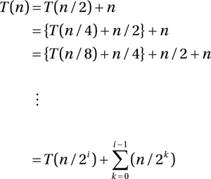
If you’re having trouble seeing how I got to the general pattern, you might want to ponder it for a minute. Basically, I’ve just used the sigma notation to express the sum n + n/2 + ... + n/(2i–1), which you can see emerging in the early unraveling steps. Before worrying about solving the sum, we once again set i = lg n. Assuming that T (1) = 1, we get the following:
The last step there is just because n/2lg n = 1, so we can include the lonely 1 into the sum.
Now: Does this sum look familiar? Once again, take a look at Figure 3-5: If k is a height, then n/2k is the number of nodes at that height (we’re halving our way from the leaves to the root). That means the sum is equal to the number of nodes, which is Θ(n).
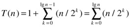
Recurrences 7 and 8 introduce a wrinkle: multiple recursive calls. Recurrence 7 is similar to recurrence 5: Instead of counting the nodes on one path from root to leaves, we now follow both child edges from each node, so the count is equal to the number of nodes, or Θ(n). Can you see how recurrences 6 and 7 are just counting the same nodes in two different ways? I’ll use our solution method on recurrence 8; the procedure for number 7 is very similar but worth checking:
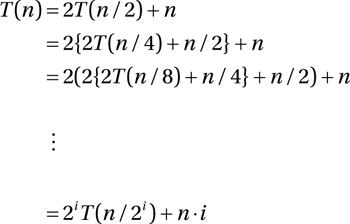
As you can see, the twos keep piling up in front, resulting in the factor of 2i. The situation does seem a bit messy inside the parentheses, but luckily, the halvings and doublings even out perfectly: The n/2 is inside the first parentheses and is multiplied by 2; n/4 is multiplied by 4, and in general, n/2i is multiplied by 2i, meaning that we’re left with a sum of i repetitions of n, or simply n·i. Once again, to get the base case, we choose i = lg n:

In other words, the running time is Θ(n lg n). Can even this result be seen in Figure 3-5? You bet! The work in the root node of the recursion tree is n; in each of the two recursive calls (the child nodes), this is halved. In other words, the work in each node is equal to the labels in Figure 3-5. We know that each row then sums to n, and we know there are lg n + 1 rows of nodes, giving us a grand sum of n lg n + n, or Θ(n lg n).
Guessing and Checking
Both recursion and induction will be discussed in depth in Chapter 4. One of my main theses there is that they are like mirror images of one another; one perspective is that induction shows you why recursion works. In this section, I restrict the discussion to showing that our solutions to recurrences are correct (rather than discussing the recursive algorithms themselves), but it should still give you a glimpse of how these things are connected.
As I said earlier in this chapter, the process of unraveling a recurrence and “finding” a pattern is somewhat subject to unwarranted assumption. For example, we often assume that n is an integer power of two so that a recursion depth of exactly lg n is attainable. In most common cases, these assumptions work out just fine, but to be sure that a solution is correct, you should check it. The nice thing about being able to check the solution is that you can just conjure up a solution by guesswork or intuition and then (ideally) show that it’s right.
Note To keep things simple, I’ll stick to the Big Oh in the following and work with upper limits. You can show the lower limits (and get Ω or Θ) in a similar manner.
Let’s take our first recurrence, T (n) = T (n–1) + 1. We want to check whether it’s correct that T (n) is O(n). As with experiments (discussed in Chapter 1), we can’t really get where we want with asymptotic notation; we have to be more specific and insert some constants, so we try to verify that T (n) ≤ cn, for some an arbitrary c ≥ 1. Per our standard assumptions, we set T(1) = 1. So far, so good. But what about larger values for n?
This is where the induction comes in. The idea is quite simple: We start with T (1), where we know our solution is correct, and then we try to show that it also applies to T (2), T (3), and so forth. We do this generically by proving an induction step, showing that if our solution is correct for T (n–1), it will also be true for T(n), for n > 1. This step would let us go from T(1) to T (2), from T (2) to T (3), and so forth, just like we want.
The key to proving an inductive step is the assumption (in this case) that we’ve got it right for T (n–1). This is precisely what we use to get to T(n), and it’s called the inductive hypothesis. In our case, the inductive hypothesis is that T (n–1) ≤ c(n–1) (for some c), and we want to show that this carries over to T(n):
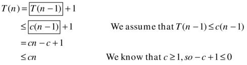
I’ve highlighted the use of the induction hypotheses with boxes here: I replace T(n–1) with c(n–1), which (by the induction hypothesis) I know is a greater (or equally great) value. This makes the replacement safe, as long as I switch from an equality sign to “less than or equal” between the first and second lines. Some basic algebra later, and I’ve shown that the assumption T(n–1) ≤ c(n–1) leads to T(n) ≤ cn, which (consequently) leads to T(n+1) ≤ c(n+1), and so forth. Starting at our base case, T(1), we have now shown that T(n) is, in general, O (n).
The basic divide and conquer recurrences aren’t much harder. Let’s do recurrence 8 (from Table 3-1). This time, let’s use something called strong induction. In the previous example, I only assumed something about the previous value (n–1, so-called weak induction); now, my induction hypothesis will be about all smaller numbers. More specifically, I’ll assume that T(k) ≤ ck lg k for all positive integers k < n and show that this leads to T(n) ≤ cn lg n. The basic idea is still the same—our solution will still “rub off” from T(1) to T(2), and so forth—it’s just that we get a little bit more to work with. In particular, we now hypothesize something about T(n/2) as well, not just T(n–1). Let’s have a go:
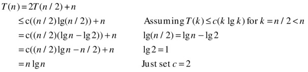
As before, by assuming that we’ve already shown our result for smaller parameters, we show that it also holds for T(n).
Caution Be wary of asymptotic notation in recurrences, especially for the recursive part. Consider the following (false) “proof” that T (n) = 2T (n/2) + n means that T(n) is O (n), using the Big Oh directly in our induction hypothesis:
T (n) = 2 · T (n/2) + n = 2 · O (n/2) + n = O (n)
There are many things wrong with this, but the most glaring problem is, perhaps, that the induction hypothesis needs to be specific to individual values of the parameter (k = 1, 2...), but asymptotic notation necessarily applies to the entire function.
DOWN THE RABBIT HOLE (OR CHANGING OUR VARIABLE)
A word of warning: The material in this sidebar may be a bit challenging. If you already have your head full with recurrence concepts, it might be a good idea to revisit it at a later time.
In some (probably rare) cases, you may come across a recurrence that looks something like the following:
T(n) = aT(n1/b) + f(n)
In other words, the subproblem sizes are b-roots of the original. Now what do you do? Actually, we can move into “another world” where the recurrence is easy! This other world must, of course, be some reflection of the real world, so we can get a solution to the original recurrence when we come back.
Our “rabbit hole” takes the form of what is called a variable change. It’s actually a coordinated change, where we replace both T (to, say, S) and n (to m) so that our recurrence is really the same as before—we’ve just written it in a different way. What we want is to change T(n1/b) into S(m/b), which is easier to work with. Let’s try a specific example, using a square root:
T(n) = 2T(n1/2) + lg n
How can we get T(n1/2) = S(m/2)? A hunch might tell us that to get from powers to products, we need to involve logarithms. The trick here is to set m = lg n, which in turn lets us insert 2m instead of n in the recurrence:
T(2m) = 2T((2m)1/2) + m = 2T(2m/2) + m
By setting S(m) = T(2m), we can hide that power, and bingo! We’re in Wonderland:
S(m) = 2S(m/2) + m
This should be easy to solve by now: T(n) = S(m) is Θ(m lg m) = Θ(lg n · lg lg n).
In the first recurrence of this sidebar, the constants a and b may have other values, of course (and f may certainly be less cooperative), leaving us with S(m) = aS(m/b) + g(m) (where g(m) = f (2m)). You could hack away at this using repeated substitution, or you could use the cookie-cutter solutions given in the next section, because they are specifically suited to this sort of recurrence.
The Master Theorem: A Cookie-Cutter Solution
Recurrences corresponding to many of so-called divide and conquer algorithms (discussed in Chapter 6) have the following form (where a ≥ 1 and b > 1):
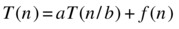
The idea is that you have a recursive calls, each on a given percentage (1/b) of the dataset. In addition to the recursive calls, the algorithm does f (n) units of work. Take a look at Figure 3-6, which illustrates such an algorithm. In our earlier trees, the number 2 was all-important, but now we have two important constants, a and b. The problem size allotted to each node is divided by b for each level we descend; this means that in order to reach a problem size of 1 (in the leaves), we need a height of logb n. Remember, this is the power to which b must be raised in order to get n.
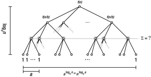
Figure 3-6. A perfectly balanced, regular multiway (a-way) tree illustrating divide and conquer recurrences
However, each internal node has a children, so the increase in the node count from level to level doesn’t necessarily counteract the decrease in problem size. This means that the number of leaf nodes won’t necessarily be n. Rather, the number of nodes increases by a factor a for each level, and with a height of logb n, we get a width of alogb n. However, because of a rather convenient calculation rule for logarithms, we’re allowed to switch a and n, yielding nlogb a leaves. Exercise 3-10 asks you to show that this is correct.
The goal in this section is to build three cookie-cutter solutions, which together form the so-called master theorem. The solutions correspond to three possible scenarios: Either the majority of the work is performed (that is, most of the time is spent) in the root node, it is primarily performed in the leaves, or it is evenly distributed among the rows of the recursion tree. Let’s consider the three scenarios one by one.
In the first scenario, most of the work is performed in the root, and by “most” I mean that it dominates the running time asymptotically, giving us a total running time of Θ(f(n)). But how do we know that the root dominates? This happens if the work shrinks by (at least) a constant factor from level to level and if the root does more work (asymptotically) than the leaves. More formally:
for some c < 1 and large n, and
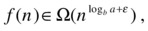
for some constant ε>0. This just means that f (n) grows strictly faster than the number of leaves (which is why I’ve added the ε in the exponent of the leaf count formula). Take, for example, the following:
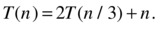
Here, a = 2, b = 3 and f(n) = n. To find the leaf count, we need to calculate log3 2. We could do this by using the expression log 2/log 3 on a standard calculator, but in Python we can use the log function from the math module, and we find that log(2,3) is a bit less than 0.631. In other words, we want to know whether f (n) = n is Ω(n0.631), which it clearly is, and this tells us that T(n) is Θ(f (n)) = Θ(n). A shortcut here would be to see that b was greater than a, which could have told us immediately that n was the dominating part of the expression. Do you see why?
We can turn the root-leaf relationship on its head as well:
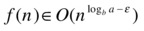
Now the leaves dominate the picture. What total running time do you think that leads to? That’s right:
Take, for example, the following recurrence:
Here a = b, so we get a leaf count of n, which clearly grows asymptotically faster than f (n) = lg n. This means that the final running time is asymptotically equal to the leaf count, or Θ(n).
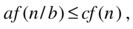
Note To establish dominance for the root, we needed the extra requirement af(n/b) ≤ cf (n), for some c < 1. To establish leaf dominance, there is no similar requirement.
The last case is where the work in the root and the leaves has the same asymptotic growth:
This then becomes the sum of every level of the tree (it neither increases nor decreases from root to leaves), which means that we can multiply it by the logarithmic height to get the total sum:
Take, for example, the following recurrence:
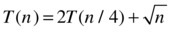
The square root may seem intimidating, but it’s just another power, namely, n0.5. We have a = 2 and b = 4, giving us logb a = log4 2 = 0.5. What do you know—the work is Θ(n0.5) in both the root and the leaves, and therefore in every row of the tree, yielding the following total running time:
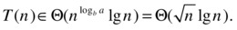
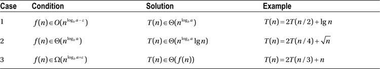
Table 3-2 sums up the three cases of the master theorem, in the order they are customarily given: Case 1 is when the leaves dominate; case 2 is the “dead race,” where all rows have the same (asymptotic) sum; and in case 3, the root dominates.
Table 3-2. The Three Cases of the Master Theorem
So What Was All That About?
OK, there is a lot of math here but not a lot of coding so far. What’s the point of all these formulas? Consider, for a moment, the Python programs in Listings 3-1 and 3-2.7 (You can find a fully commented version of the mergesort function in Listing 6-6.) Let’s say these were new algorithms, so you couldn’t just search for their names on the Web, and your task was to determine which had the better asymptotic running time complexity.
Listing 3-1. Gnome Sort, An Example Sorting Algorithm
def gnomesort(seq):
    i = 0
    while i < len(seq):
        if i == 0 or seq[i-1] <= seq[i]:
            i += 1
        else:
            seq[i], seq[i-1] = seq[i-1], seq[i]
            i -= 1
Listing 3-2. Merge Sort, Another Example Sorting Algorithm
def mergesort(seq):
    mid = len(seq)//2
    lft, rgt = seq[:mid], seq[mid:]
    if len(lft) > 1: lft = mergesort(lft)
    if len(rgt) > 1: rgt = mergesort(rgt)
    res = []
    while lft and rgt:
        if lft[-1] >=rgt[-1]:
            res.append(lft.pop())
        else:
            res.append(rgt.pop())
    res.reverse()
    return (lft or rgt) + res
Gnome sort contains a single while loop and an index variable that goes from 0 to len(seq)-1, which might tempt us to conclude that it has a linear running time, but the statement i -= 1 in the last line would indicate otherwise. To figure out how long it runs, you need to understand something about how it works. Initially, it scans from a from the left (repeatedly incrementing i), looking for a position i where seq[i-1] is greater than seq[i], that is, two values that are in the wrong order. At this point, the else part kicks in.
The else clause swaps seq[i] and seq[i-1] and decrements i. This behavior will continue until, once again, seq[i-1] <= seq[i] (or we reach position 0) and order is restored. In other words, the algorithm alternately scans upward in the sequence for an out-of-place (that is, too small) element and moves that element down to a valid position by repeated swapping. What’s the cost of all this? Let’s ignore the average case and focus on the best and worst. The best case occurs when the sequence is sorted: gnomesort will just scan through a without finding anything out of place and then terminate, yielding a running time of Θ(n).
The worst case is a little less straightforward but not much. Note that once we find an element that is out of place, all elements before that point are already sorted, and moving the new element into a correct position won’t scramble them. That means the number of sorted elements will increase by one each time we discover a misplaced element, and the next misplaced element will have to be further to the right. The worst possible cost of finding and moving a misplaced element into place is proportional to its position, so the worst running time could possibly get is 1 + 2 + ... + n–1, which is Θ(n2). This is a bit hypothetical at the moment—I’ve shown it can’t get worse than this, but can it ever get this bad?
Indeed it can. Consider the case when the elements are sorted in descending order (that is, reversed with respect to what we want). Then every element is in the wrong place and will have to be moved all the way to the start, giving us the quadratic running time. So, in general, the running time of gnome sort is Ω(n) and O(n2), and these are tight bounds representing the best and worst cases, respectively.
Now, take a look at merge sort (Listing 3-2). It is a bit more complicated than gnome sort, so I’ll postpone explaining how it manages to sort things until Chapter 6. Luckily, we can analyze its running time without understanding how it works! Just look at the overall structure. The input (seq) has a size of n. There are two recursive calls, each on a subproblem of n/2 (or as close as we can get with integer sizes). In addition, there is some work performed in a while loop and in res.reverse(); Exercise 3-11 asks you to show that this work is Θ(n). (Exercise 3-12 asks you what happens if you use pop(0) instead of pop().) This gives us the well-known recurrence number 8, T(n) = 2T(n/2) + Θ(n), which means that the running time of merge sort is Θ(n lg n), regardless of the input. This means that if we’re expecting the data to be almost sorted, we might prefer gnome sort, but in general we’d probably be much better off scrapping it in favor of merge sort.
Note Python’s sorting algorithm, timsort, is a naturally adaptive version of merge sort. It manages to achieve the linear best-case running time while keeping the loglinear worst case. You can find some more details in the “Black Box” sidebar on timsort in Chapter 6.
Summary
The sum of the n first integers is quadratic, and the sum of the lg n first powers of two is linear. The first of these identities can be illustrated as a round-robin tournament, with all possible pairings of n elements; the second is related to a knockout tournament, with lg n rounds, where all but the winner must be knocked out. The number of permutations of n is n!, while the number of k-combinations (subsets of size k) from n, written C(n, k), is n!/(k!·(n–k)!). This is also known as the binomial coefficient.
A function is recursive if it calls itself (directly or via other functions). A recurrence relation is an equation that relates a function to itself, in a recursive way (such as T(n) = T(n/2) + 1). These equations are often used to describe the running times of recursive algorithms, and to be able to solve them, we need to assume something about the base case of the recursion; normally, we assume that T(k) is Θ(1), for some constant k. This chapter presents three main ways of solving recurrences: (1) repeatedly apply the original equation to unravel the recursive occurrences of T until you find a pattern; (2) guess a solution, and try to prove that it’s correct using induction; and (3) for divide and conquer recurrences that fit one of the cases of the master theorem, simply use the corresponding solution.
If You’re Curious ...
The topics of this chapter (and the previous, for that matter) are commonly classified as part of what’s called discrete mathematics.8 There are plenty of books on this topic, and most of the ones I’ve seen have been pretty cool. If you like that sort of thing, knock yourself out at the library or at a local or online bookstore. I’m sure you’ll find plenty to keep you occupied for a long time.
One book I like that deals with counting and proofs (but not discrete math in general) is Proofs That Really Count, by Benjamin and Quinn. It’s worth a look. If you want a solid reference that deals with sums, combinatorics, recurrences, and lots of other meaty stuff, specifically written for computer scientists, you should check out the classic Concrete Mathematics, by Graham, Knuth, and Patashnik. (Yeah, it’s that Knuth, so you know it’s good.) If you just need some place to look up the solution for a sum, you could try Wolfram Alpha (http://wolframalpha.com), as mentioned earlier, or get one of those pocket references full of formulas (again, probably available from your favorite bookstore).
If you want more details on recurrences, you could look up the standard methods in one of the algorithm textbooks I mentioned in Chapter 1, or you could research some of the more advanced methods, which let you deal with more recurrence types than those I’ve dealt with here. For example, Concrete Mathematics explains how to use so-called generating functions. If you look around online, you’re also bound to find lots of interesting stuff on solving recurrences with annihilators or using the Akra-Bazzi theorem.
The sidebar on pseudopolynomiality earlier in this chapter used primality checking as an example. Many (older) textbooks claim that this is an unsolved problem (that is, that there are no known polynomial algorithms for solving it). Just so you know—that’s not true anymore: In 2002, Agrawal, Kayal, and Saxena published their groundbreaking paper “PRIMES is in P,” describing how to do polynomial primality checking. (Oddly enough, factoring numbers is still an unsolved problem.)
Exercises
3-1. Show that the properties described in the section “Working with Sums” are correct.
3-2. Use the rules from Chapter 2 to show that n(n–1)/2 is Θ(n2).
3-3. The sum of the first k non-negative integer powers of 2 is 2k+1 – 1. Show how this property lets you represent any positive integer as a binary number.
3-4. In the section “The Hare and the Tortoise,” two methods of looking for a number are sketched. Turn these methods into number-guessing algorithms, and implement them as Python programs.
3-5. Show that C(n, k) = C(n, n–k).
3-6. In the recursive function S early in the section “Recursion and Recurrences,” assume that instead of using a position parameter, i, the function simply returned sec[0] + S(seq[1:]). What would the asymptotic running time be now?
3-7. Solve recurrence 2 in Table 3-1 using repeated substitution.
3-8. Solve recurrence 3 in Table 3-1 using repeated substitution.
3-9. Solve recurrence 4 in Table 3-1 using repeated substitution.
3-10. Show that xlog y = ylog x, no matter the base of the logarithm.
3-11. Show that f (n) is Θ(n) for the implementation of merge sort in Listing 3-2.
3-12. In merge sort in Listing 3-2, objects are popped from the end of each half of the sequence (with pop()). It might be more intuitive to pop from the beginning, with pop(0), to avoid having to reverse res afterward (I’ve seen this done in real life), but pop(0), just like insert(0), is a linear operation, as opposed to pop(), which is constant. What would such a switch mean for the overall running time?
References
Agrawal, M., Kayal, N., and Saxena, N. (2004). PRIMES is in P. The Annals of Mathematics, 160(2):781–793.
Akra, M. and Bazzi, L. (1998). On the solution of linear recurrence equations. Computational Optimization and Applications, 10(2):195–210.
Benjamin, A. T. and Quinn, J. (2003). Proofs that Really Count: The Art of Combinatorial Proof. The Mathematical Association of America.
Graham, R. L., Knuth, D. E., and Patashnik, O. (1994). Concrete Mathematics: A Foundation for Computer Science, second edition. Addison-Wesley Professional.
__________________
1As long as the functions don’t have any side effects, that is, but behave like mathematical functions.
2http://prb.org/Articles/2002/HowManyPeoplehaveEverLivedonEarth.aspx.
3If this were true, the human population would have consisted of one man and one woman about 32 generations ago ... but, as I said, play along.
4Reportedly, this is the reward that the creator of chess asked for and was granted ... although he was told to count each grain he received. I’m guessing he changed his mind.
5Do you see where the –1 in the exponent went? Remember, 2a+b = 2a · 2b...
6Another thing that’s not immediately obvious is where the name “binomial coefficient” comes from. You might want to look it up. It’s kind of neat.
7Merge sort is a classic, first implemented by computer science legend John von Neumann on the EDVAC in 1945. You’ll learn more about that and other similar algorithms in Chapter 6. Gnome sort was invented in 2000 by Hamid Sarbazi-Azad, under the name Stupid sort.
8If you’re not sure about the difference between discrete and discreet, you might want to look it up.