Table of Contents for
Python Algorithms: Mastering Basic Algorithms in the Python Language, Second Edition
 Python Algorithms: Mastering Basic Algorithms in the Python Language, Second Edition
Published by
Apress, 2015
Python Algorithms: Mastering Basic Algorithms in the Python Language, Second Edition
Published by
Apress, 2015
- Cover
- Title
- Copyright
- Dedication
- Contents at a Glance
- Contents
- About the Author
- About the Technical Reviewer
- Acknowledgments
- Preface
- Chapter 1: Introduction
- Chapter 2: The Basics
- Chapter 3: Counting 101
- Chapter 4: Induction and Recursion … and Reduction
- Chapter 5: Traversal: The Skeleton Key of Algorithmics
- Chapter 6: Divide, Combine, and Conquer
- Chapter 7: Greed Is Good? Prove It!
- Chapter 8: Tangled Dependencies and Memoization
- Chapter 9: From A to B with Edsger and Friends
- Chapter 10: Matchings, Cuts, and Flows
- Chapter 11: Hard Problems and (Limited) Sloppiness
- Appendix A: Pedal to the Metal: Accelerating Python
- Appendix B: List of Problems and Algorithms
- Appendix C: Graph Terminology
- Appendix D: Hints for Exercises
- Index

Greed Is Good? Prove It!
It’s not a question of enough, pal.
— Gordon Gekko, Wall Street
So-called greedy algorithms are short-sighted, in that they make each choice in isolation, doing what looks good right here, right now. In many ways, eager or impatient might be better names for them because other algorithms also usually try to find an answer that is as good as possible; it’s just that the greedy ones take what they can get at this moment, not worrying about the future. Designing and implementing a greedy algorithm is usually easy, and when they work, they tend to be highly efficient. The main problem is showing that they do work—if, indeed, they do. That’s the reason for the “Prove It!” part of the chapter title.
This chapter deals with greedy algorithms that give correct (optimal) answers; I’ll revisit the design strategy in Chapter 11, where I’ll relax this requirement to “almost correct (optimal).”
Staying Safe, Step by Step
The common setting for greedy algorithms is a series of choices (just like, as you’ll see, for dynamic programming). The greed involves making each choice with local information, doing what looks most promising without regard for context or future consequences, and then, once the choice has been made, never looking back. If this is to lead to a solution, we must make sure that each choice is safe—that it doesn’t destroy our future prospects. You’ll see many examples of how we can ensure this kind of safety (or, rather, how we can prove that an algorithm is safe), but let’s start out by looking at the “step by step” part.
The kind of problems solved with greedy algorithms typically build a solution gradually. It has a set of “solution pieces” that can be combined into partial, and eventually complete, solutions. These pieces can fit together in complex ways; there may be many ways of combining them, and some pieces may no longer fit once we’ve used certain others. You can think of this as a jigsaw puzzle with many possible solutions (see Figure 7-1). The jigsaw picture is blank, and the puzzle pieces are rather regular, so they can be used in several locations and combinations.
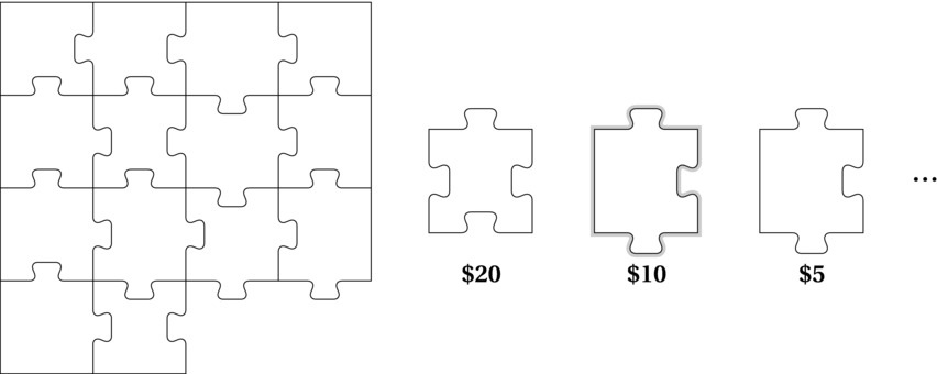
Figure 7-1. A partial solution, and some greedily ordered pieces (considered from left to right), with the next greedy choice highlighted
Now add a value to each puzzle piece. This is an amount you’ll be awarded for fitting that particular piece into the complete solution. The goal is then to find a way to lay the jigsaw that gets you the highest total value—that is, we have an optimization problem. Solving a combinatorial optimization problem like this is, in general, not at all a simple task. You might need to consider every possible way of placing the pieces, yielding an exponential (possibly factorial) running time.
Let’s say you’re filling in the puzzle row by row, from the top, so you always know where the next piece must go. The greedy approach in this setting is as easy as it gets, at least for selecting the pieces to use. Just sort the pieces by decreasing value and consider them one by one. If a piece won’t fit, you discard it. If it fits, you use it, without regard for future pieces.
Even without looking at the issue of correctness (or optimality), it’s clear that this kind of algorithm needs a couple of things to be able to run at all:
- A set of candidate elements, or pieces, with some value attached
- A way of checking whether a partial solution is valid, or feasible
So, partial solutions are built as collections of solution pieces. We check each piece in turn, starting with the most valuable one, and add each piece that leads to a larger, still valid solution. There are certainly subtleties that could be added to this (for example, the total value needn’t be a sum of element values, and we might want to know when we’re done, without having to exhaust the set of elements), but this’ll do as a prototypical description.
A simple example of this kind of problem is that of making change—trying to add up to a given sum with as few coins and bills as possible. For example, let’s say someone owes you $43.68 and gives you a hundred-dollar bill. What do you do? The reason this problem is a nice example is that we all instinctively know the right thing to do here1: We start with the biggest denominations possible and work our way down. Each bill or coin is a puzzle piece, and we’re trying to cover the number $56.32 exactly. Instead of sorting a set of bills and coins, we can think of sorting stacks of them, because we have many of each. We sort these stacks in descending order and start handing out the largest denominations, like in the following code (working with cents, to avoid floating-point issues):
>>> denom = [10000, 5000, 2000, 1000, 500, 200, 100, 50, 25, 10, 5, 1]
>>> owed = 5632
>>> payed = []
>>> for d in denom:
...     while owed >=d:
...         owed -= d
...         payed.append(d)
...
>>> sum(payed)
5632
>>> payed
[5000, 500, 100, 25, 5, 1, 1]
Most people probably have little doubt that this works; it seems like the obvious thing to do. And, indeed, it works, but the solution is in some ways very brittle. Even changing the list of available denominations in minor ways will destroy it (see Exercise 7-1). Figuring out which currencies the greedy algorithm will work with isn’t straightforward (although there is an algorithm for it), and the general problem itself is unsolved. In fact, it’s closely related to the knapsack problem, which is discussed in the next section.
Let’s turn to a different kind of problem, related to the matching we worked with in Chapter 4. The movie is over (with many arguing that the TV show was clearly superior), and the group decides to go out for some tango, and once again, they face a matching problem. Each pair of people has a certain compatibility, which they’ve represented as a number, and they want the sum of these over all the pairs to be as high as possible. Dance pairs of the same gender are not uncommon in tango, so we needn’t restrict ourselves to the bipartite case—and what we end up with is the maximum-weight matching problem. In this case (or the bipartite case, for that matter), greed won’t work in general. However, by some freak coincidence, all the compatibility numbers happen to be distinct powers of two. Now, what happens?2
Let’s first consider what a greedy algorithm would look like here and then see why it yields an optimal result. We’ll be building a solution piece by piece—let the pieces be all the possible pairs and a partial solution be a set of pairs. Such a partial solution is valid only if everyone participates in at most one of its pairs. The algorithm will then be roughly as follows:
- List potential pairs, sorted by decreasing compatibility.
- Pick the first unused pair from the list.
- Is anyone in the pair already occupied? If so, discard it; otherwise, use it.
- Are there any more pairs on the list? If so, go to 2.
As you’ll see later, this is rather similar to Kruskal’s algorithm for minimum spanning trees (although that works regardless of the edge weights). It also is a rather prototypical greedy algorithm. Its correctness is another matter. Using distinct powers of two is sort of cheating because it would make virtually any greedy algorithm work; that is, you’d get an optimal result as long as you could get a valid solution at all (see Exercise 7-3). Even though it’s cheating, it illustrates the central idea here: making the greedy choice is safe. Using the most compatible of the remaining couples will always be at least as good as any other choice.3
In the following sections, I’ll show you some well-known problems that can be solved using greedy algorithms. For each algorithm, you’ll see how it works and why greed is correct. Near the end of the chapter, I’ll sum up some general approaches to proving correctness that you can use for other problems.
EAGER SUITORS AND STABLE MARRIAGES
There is, in fact, one classical matching problem that can be solved (sort of) greedily: the stable marriage problem. The idea is that each person in a group has preferences about whom he or she would like to marry. We’d like to see everyone married, and we’d like the marriages to be stable, meaning that there is no man who prefers a woman outside his marriage who also prefers him. (To keep things simple, we disregard same-sex marriages and polygamy here.)
There’s a simple algorithm for solving this problem, designed by David Gale and Lloyd Shapley. The formulation is quite gender-conservative but will certainly also work if the gender roles are reversed. The algorithm runs for a number of rounds, until there are no unengaged men left. Each round consists of two steps:
- Each unengaged man proposes to his favorite of the women he has not yet asked.
- Each woman is (provisionally) engaged to her favorite suitor and rejects the rest.
This can be viewed as greedy in that we consider only the available favorites (both of the men and women) right now. You might object that it’s only sort of greedy in that we don’t lock in and go straight for marriage; the women are allowed to break their engagement if a more interesting suitor comes along. Even so, once a man has been rejected, he has been rejected for good, which means that we’re guaranteed progress and a quadratic worst-case running time.
To show that this is an optimal and correct algorithm, we need to know that everyone gets married and that the marriages are stable. Once a woman is engaged, she stays engaged (although she may replace her fiancé). There is no way we can get stuck with an unmarried pair, because at some point the man would have proposed to the woman, and she would have (provisionally) accepted his proposal.
How do we know the marriages are stable? Let’s say Scarlett and Stuart are both married but not to each other. Is it possible they secretly prefer each other to their current spouses? No. If this were so, Stuart would already have proposed to her. If she accepted that proposal, she must later have found someone she liked better; if she rejected it, she would already have a preferable mate.
Although this problem may seem silly and trivial, it is not. For example, it is used for admission to some colleges and to allocate medical students to hospital jobs. There are, in fact, entire books (such as those by Donald Knuth and by Dan Gusfield and Robert W. Irwing) devoted to the problem and its variations.

All the Girls. You know that I’ll never leave you. Not as long as she’s with someone. (http://xkcd.com/770)
The Knapsack Problem
This problem is, in a way, a generalization of the change-making problem, discussed earlier. In that problem, we used the coin denominations to determine whether a partial/full solution was valid (don’t give too much/give the exact amount), and the number of coins measured the quality of the eventual solution. The knapsack problem is framed in different terms: We have a set of items that we want to take with us, each with a certain weight and value; however, our knapsack has a maximum capacity (an upper bound on the total weight), and we want to maximize the total value we get.
The knapsack problem covers many applications. Whenever you are to select a valuable set of objects (memory blocks, text fragments, projects, people), where each object has an individual value (possibly be linked to money, probability, recency, competence, relevance, or user preferences), but you are constrained by some resource (be it time, memory, screen real-estate, weight, volume or something else entirely), you may very well be solving a version of the knapsack problem. There are also special cases and closely related problems, such as the subset sum problem, discussed in Chapter 11, and the problem of making change, as discussed earlier. This wide applicability is also its weakness—what makes it such a hard problem to solve. As a rule, the more expressive a problem is, the harder it is to find an efficient algorithm for it. Luckily, there are special cases that we can solve in various ways, as you’ll see in the following sections.
Fractional Knapsack
This is the simplest of the knapsack problems. Here we’re not required to include or exclude entire objects; we might be stuffing our backpack with tofu, whiskey, and gold dust, for example (making for a somewhat odd picnic). We needn’t allow arbitrary fractions, though. We could, for example, use a resolution of grams or ounces. (We could be even more flexible; see Exercise 7-6.) How would you approach this problem?
The important thing here is to find the value-to-weight ratio. For example, most people would agree that gold dust has the most value per gram (though it might depend on what you’d use it for); let’s say the whiskey falls between the two (although I’m sure there are those who’d dispute that). In that case, to get the most out of our backpack, we’d stuff it full with gold dust—or at least with the gold dust we have. If we run out, we start adding the whiskey. If there’s still room left over when we’re out of whiskey, we top it all off with tofu (and start dreading the unpacking of this mess).
This is a prime example of a greedy algorithm. We go straight for the good (or, at least, expensive) stuff. If we use a discrete weight measure, this can, perhaps, be even easier to see; that is, we don’t need to worry about ratios. We basically have a set of individual grams of gold dust, whiskey, and tofu, and we sort them according to their value. Then, we (conceptually) pack the grams one by one.
Integer Knapsack
Let’s say we abandon the fractions, and now need to include entire objects—a situation more likely to occur in real life, whether you’re programming or packing your bag. Then the problem is suddenly a lot harder to solve. For now, let’s say we’re still dealing with categories of objects, so we can add an integer amount (that is, number of objects) from each category. Each category then has a fixed weight and value that holds for all objects. For example, all gold bars weigh the same and have the same value; the same holds for bottles of whiskey (we stick to a single brand) and packages of tofu. Now, what do we do?
There are two important cases of the integer knapsack problem—the bounded and unbounded cases. The bounded case assumes we have a fixed number of objects in each category,4 and the unbounded case lets us use as many as we want. Sadly, greed won’t work in either case. In fact, these are both unsolved problems, in the sense that no polynomial algorithms are known to solve them in general. There is hope, however. As you’ll see in the next chapter, we can use dynamic programming to solve the problems in pseudopolynomial time, which may be good enough in many important cases. Also, for the unbounded case, it turns out that the greedy approach ain’t half bad! Or, rather, it’s at least half good, meaning we’ll never get less than half the optimum value. And with a slight modification, you can get as good results for the bounded version, too. This concept of greedy approximation is discussed in more detail in Chapter 11.
 Note This is mainly an initial “taste” of the knapsack problem. I’ll deal more thoroughly with a solution to the integer knapsack problem in Chapter 8.
Huffman’s Algorithm
Huffman’s algorithm is another one of the classics of greed. Let’s say you’re working with some emergency central where people call for help. You’re trying to put together some simple yes/no questions that can be posed in order to help the callers diagnose an acute medical problem and decide on the appropriate course of action. You have a list of the conditions that should be covered, along with a set of diagnostic criteria, severity, and frequency of occurrence. Your first thought is to build a balanced binary tree, constructing a question in each node that will split the list (or sublist) of possible conditions in half. This seems too simplistic, though; the list is long and includes many noncritical conditions. Somehow, you need to take severity and frequency of occurrence into account.
It’s usually a good idea to simplify any problem at first, so you decide to focus on frequency. You realize that the balanced binary tree is based on the assumption of uniform probability—dividing the list in half won’t do if some items are more probable. If, for example, there’s an even chance that the patient is unconscious, that’s the thing to ask about—even if “Does the patient have a rash?” might actually split the list in the middle. In other words, you want a weighted balancing: You want the expected number of questions to be as low as possible. You want to minimize the expected depth of your (pruned) traversal from root to leaf.
You find that this idea can be used to account for the severity as well. You’d want to prioritize the most dangerous conditions so they can be identified quickly (“Is the patient breathing?”), at the cost of making patients with less critical ailments wait through a couple of extra questions. You do this, with the help of some health professionals, by giving each condition a cost or weight, combining the frequency (probability) and the health risk involved. Your goal for the tree structure is still the same. How can you minimize the sum of depth(u) × weight(u) over all leaves u?
This problem certainly has other applications as well. In fact, the original (and most common) application is compression—representing a text more compactly—through variable-length codes. Each character in your text has a frequency of occurrence, and you want to exploit this information to give the characters encodings of different lengths so as to minimize the expected length of any text. Equivalently, for any character, you want to minimize the expected length of its encoding.
Do you see how this is similar to the previous problem? Consider the version where you focused only on the probability of a given medical condition. Now, instead of minimizing the number of yes/no questions needed to identify some medical affliction, we want to minimize the number of bits needed to identify a character. Both the yes/no answers and the bits uniquely identify paths to leaves in a binary tree (for example, zero = no = left and one = yes = right).5 For example, consider the characters a through f. One way of encoding them is given by Figure 7-2 (just ignore the numbers in the nodes for now). For example, the code for g (given by the highlighted path) would be 101. Because all characters are in the leaves, there would be no ambiguity when decoding a text that had been compressed with this scheme (see Exercise 7-7). This property, that no valid code is a prefix of another, gives rise to the term prefix code.
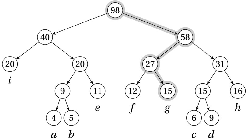
Figure 7-2. A Huffman tree for a–i, with frequencies/weights 4, 5, 6, 9, 11, 12, 15, 16, and 20, and the path represented by the code 101 (right, left, right) highlighted
The Algorithm
Let’s start by designing a greedy algorithm to solve this problem, before showing that it’s correct (which is, of course, the crucial step). The most obvious greedy strategy would, perhaps, be to add the characters (leaves) one by one, starting with the one with the greatest frequency. But where would we add them? Another way to go (which you’ll see again in Kruskal’s algorithm, in a bit) is to let a partial solution consist of several tree fragments and then repeatedly combine them. When we combine two trees, we add a new, shared root and give it a weight equal to the sum of its children, that is, the previous roots. This is exactly what the numbers inside the nodes in Figure 7-2 mean.
Listing 7-1 shows one way of implementing Huffman’s algorithm. It maintains a partial solution as a forest, with each tree represented as nested lists. For as long as there are at least two separate trees in the forest, the two lightest trees (the ones with lowest weights in their roots) are picked out, combined, and placed back in, with a new root weight.
Listing 7-1. Huffman’s Algorithm
from heapq import heapify, heappush, heappop
from itertools import count

def huffman(seq, frq):
    num = count()
    trees = list(zip(frq, num, seq))            # num ensures valid ordering
    heapify(trees)                              # A min-heap based on frq
    while len(trees) > 1:                       # Until all are combined
        fa, _, a = heappop(trees)               # Get the two smallest trees
        fb, _, b = heappop(trees)
        n = next(num)
        heappush(trees, (fa+fb, n, [a, b]))     # Combine and re-add them
    return trees[0][-1]
Here’s an example of how you might use the code:
>>> seq = "abcdefghi"
>>> frq = [4, 5, 6, 9, 11, 12, 15, 16, 20]
>>> huffman(seq, frq)
[['i', [['a', 'b'], 'e']], [['f', 'g'], [['c', 'd'], 'h']]]
A few details are worth noting in the implementation. One of its main features is the use of a heap (from heapq). Repeatedly selecting and combining the two smallest elements of an unsorted list would give us a quadratic running time (linear selection time, linear number of iterations), while using a heap reduces that to loglinear (logarithmic selection and re-addition). We can’t just add the trees directly to the heap, though; we need to make sure they’re sorted by their frequencies. We could simply add a tuple, (freq, tree), and that would work as long as all frequencies (that is, weights) were different. However, as soon as two trees in the forest have the same frequency, the heap code would have to compare the trees to see which one is smaller—and then we’d quickly run into undefined comparisons.
Note In Python 3, comparing incompatible objects like ["a", ["b", "c"]] and "d" is not allowed and will raise a TypeError. In earlier versions, this was allowed, but the ordering was generally not very meaningful; enforcing more predictable keys is probably a good thing either way.
A solution is to add a field between the two, one that is guaranteed to differ for all objects. In this case, I simply use a counter, resulting in (freq, num, tree), where frequency ties are broken using the arbitrary num, avoiding direct comparison of the (possibly incomparable) trees.6
As you can see, the resulting tree structure is equivalent to the one shown in Figure 7-2.
To compress and decompress a text using this technique, you need some pre- and post-processing, of course. First, you need to count characters to get the frequencies (for example, using the Counter class from the collections module). Then, once you have your Huffman tree, you must find the codes for all the characters. You could do this with a simple recursive traversal, as shown in Listing 7-2.
Listing 7-2. Extracting Huffman Codes from a Huffman Tree
def codes(tree, prefix=""):
    if len(tree) == 1:
        yield (tree, prefix)                    # A leaf with its code
        return
    for bit, child in zip("01", tree):          # Left (0) and right (1)
        for pair in codes(child, prefix + bit): # Get codes recursively
            yield pair
The codes function yields (char, code) pairs suitable for use in the dict constructor, for example. To use such a dict to compress a code, you’d just iterate over the text and look up each character. To decompress the text, you’d rather use the Huffman tree directly, traversing it using the bits in the input for directions (that is, determining whether you should go left or right); I’ll leave the details as an exercise for the reader.
The First Greedy Choice
I’m sure you can see that the Huffman codes will let you faithfully encode a text and then decode it again—but how can it be that it is optimal (within the class of codes we’re considering)? That is, why is the expected depth of any leaf minimized using this simple, greedy procedure?
As we usually do, we now turn to induction: We need to show that we’re safe all the way from start to finish—that the greedy choice won’t get us in trouble. We can often split this proof into two parts, what is often called (i) the greedy choice property and (ii) optimal substructure (see, for example, Cormen et al. in the “References” section of Chapter 1). The greedy choice property means that the greedy choice gives us a new partial solution that is part of an optimal one. The optimal substructure, which is very closely related to the material of Chapter 8, means that the rest of the problem, after we’ve made our choice, can also be solved just like the original—if we can find an optimal solution to the subproblem, we can combine it with our greedy choice to get a solution to the entire problem. In other words, an optimal solution is built from optimal subsolutions.
To show the greedy choice property for Huffman’s algorithm, we can use an exchange argument (see, for example, Kleinberg and Tardos in the “References” section of Chapter 1). This is a general technique used to show that our solution is at least as good as an optimal one (and therefore optimal)—or in this case, that there exists a solution with our greedy choice that is at least this good. The “at least as good” part is proven by taking a hypothetical (totally unknown) optimal solution and then gradually changing it into our solution (or, in this case, one containing the bits we’re interested in) without making it worse.
The greedy choice for Huffman’s algorithm involves placing the two lightest elements as sibling leaves on the lowest level of the tree. (Note that we’re worried about only the first greedy choice; the optimal substructure will deal with the rest of the induction.) We need to show that this is safe—that there exists an optimal solution where the two lightest elements are, indeed, bottom-level sibling leaves. Start the exchange argument by positing another optimal tree where these two elements are not lowest-level siblings. Let a and b be the lowest-frequency elements, and assume that this hypothetical, optimal tree has c and d as sibling leaves at maximum depth. We assume that a is lighter (has a lower weight/frequency) than b and that c is lighter than d.7 Under the circumstances, we also know that a is lighter than c and b is lighter than d. For simplicity, let’s assume that the frequences of a and d are different because otherwise the proof is simple (see Exercise 7-8).
What happens if we swap a and c? And then swap b and d? For one thing, we now have a and b as bottom-level siblings, which we wanted, but what has happened to the expected leaf depth? You could fiddle around with the full expressions for weighted sums here, but the simple idea is: We’ve moved some heavy nodes up in the tree and moved some light nodes down. This means that some short paths are now given a higher weight in the sum, while some long paths have been given a lower weight. All in all, the total cost cannot have increased. (Indeed, if the depths and weights are all different, our tree will be better, and we have a proof by contradiction because our hypothetical alternative optimum cannot exist—the greedy way is the best there is.)
Going the Rest of the Way
Now, that was the first half of the proof. We know that making the first greedy choice was OK (the greedy choice property), but we need to know that it’s OK to keep using greedy choices (optimal substructure). We need to get a handle on what the remaining subproblem is first, though. Preferably, we’d like it to have the same structure as the original, so the machinery of induction can do its job properly. In other words, we’d like to reduce things to a new, smaller set of elements for which we can build an optimal tree and then show how we can build on that.
The idea is to view the first two combined leaves as a new element, ignoring the fact that it’s a tree. We worry only about its root. The subproblem then becomes finding an optimal tree for this new set of elements—which we can assume is all right, by induction. The only remaining question is whether this tree is optimal once we expand this node back to a three-node subtree, by once again including its leaf children; this is the crucial part that will give us the induction step.
Let’s say our two leaves are, once again, a and b, with frequencies f(a) and f(b). We lump them together as a single node with a frequency f(a) + f(b) and construct an optimal tree. Let’s assume that this combined node ends up at depth D. Then its contribution to the total tree cost is D × (f(a) + f(b)). If we now expand the two children, their parent node no longer contributes to the cost, but the total contribution of the leaves (which are now at depth D + 1) will be (D + 1) × (f(a) + f(b)). In other words, the full solution has a cost that exceeds the optimal subsolution by f(a) + f(b). Can we be sure that this is optimal?
Yes, we can, and we can prove it by contradiction, assuming that it is not optimal. We conjure up another, better tree—and assume that it, too, has a and b as bottom-level siblings. (We know, by the arguments in the previous section, that an optimal tree like this exists.) Once again, we can collapse a and b, and we end up with a solution to our subproblem that is better than the one we had … but the one we had was optimal by assumption! In other words, we cannot find a global solution that is better than one that contains an optimal subsolution.
Optimal Merging
Although Huffman’s algorithm is normally used to construct optimal prefix codes, there are other ways of interpreting the properties of the Huffman tree. As explained initially, one could view it as a decision tree, where the expected traversal depth is minimized. We can use the weights of the internal nodes in our interpretation too, though, yielding a rather different application.
We can view the Huffman tree as a sort of fine-tuned divide-and-conquer tree, where we don’t do a flat balancing like in Chapter 6, but where the balance has been designed to take the leaf weights into account. We can then interpret the leaf weights as subproblem sizes, and if we assume that the cost of combining (merging) subproblems is linear (as is often the case in divide and conquer), the sum of all the internal node weights represents the total work performed.
A practical example of this is merging sorted files, for example. Merging two files of sizes n and m takes time linear in n+m. (This is similar to the problem of joining in relational database or of merging sequences in algorithms such as timsort.) In other words, if you imagine the leaves in Figure 7-2 to be files and their weights to be file sizes, the internal nodes represent the cost of the total merging. If we can minimize the sum of the internal nodes (or, equivalently, the sum of all the nodes), we will have found the optimal merging schedule. (Exercise 7-9 asks you to show that this really matters.)
We now need to show that a Huffman tree does, indeed, minimize the node weights. Luckily, we can piggyback this proof on the previous discussion. We know that in a Huffman tree, the sum of depth times weight over all leaves is minimized. Now, consider how each leaf contributes to the sum over all nodes: The leaf weight occurs as a summand once in each of its ancestor nodes—which means that the sum is exactly the same! That is, sum(weight(node) for node in nodes) is the same as sum(depth(leaf)*weight(leaf) for leaf in leaves). In other words, Huffman’s algorithm is exactly what we need for our optimal merging.
Tip The Python standard library has several modules dealing with compression, including zlib, gzip, bz2, zipfile, and tar. The zipfile module deals with ZIP files, which use compression that is based on, among other things, Huffman codes.8
Minimum Spanning Trees
Now let’s take a look at the perhaps most well-known example of a greedy problem: finding minimum spanning trees. The problem is an old one—it’s been around at least since the early 20th century. It was first solved by the Czech mathematician Otakar Borůvka in 1926, in an effort to construct a cheap electrical network for Moravia. His algorithm has been rediscovered many times since then, and it still forms the basis of some of the fastest known algorithms known today. The algorithms I’ll discuss in this section (Prim’s and Kruskal’s) are in some way a bit simpler but have the same asymptotic running time complexity (O(m lg n), for n nodes and m edges).9 If you’re interested in the history of this problem, including the repeated rediscoveries of the classic algorithms, take a look at the paper “On the History of the Minimum Spanning Tree Problem,” by Graham and Hell. (For example, you’ll see that Prim and Kruskal aren’t the only ones to lay claim to their eponymous algorithms.)
We’re basically looking for the cheapest way of connecting all the nodes of a weighted graph, given that we can use only a subset of its edges to do the job. The cost of a solution is simply the weight sum for the edges we use.10 This could be useful in building an electrical grid, constructing the core of a road or railroad network, laying out a circuit, or even performing some forms of clustering (where we’d only almost connect all the nodes). A minimum spanning tree can also be used as a foundation for an approximate solution to the traveling salesrep problem introduced in Chapter 1 (see Chapter 11 for a discussion on this).
A spanning tree T of a connected, undirected graph G has the same node set as G and a subset of the edges. If we associate an edge weight function with G so edge e has weight w(e), then the weight of the spanning tree, w(T), is the sum of w(e) for every edge e in T. In the minimum spanning tree problem, we want to find a spanning tree over G that has minimum weight. (Note that there may be more than one.) Note also that if G is disconnected, it will have no spanning trees, so in the following, it is generally assumed that the graphs we’re working with are connected.
In Chapter 5, you saw how to build spanning trees using traversal; building minimum spanning trees can also be built in an incremental step like this, and that’s where the greed comes in: We gradually build the tree by adding one edge at the time. At each step, we choose the cheapest (or lightest) edge among those permitted by our building procedure. This choice is locally optimal (that is, greedy) and irrevocable. The main task for this problem, or any other greedy problem, becomes showing that these locally optimal choices lead to a globally optimal solution.
The Shortest Edge
Consider Figure 7-3. Let the edge weights correspond to the Euclidean distances between the nodes as they’re drawn (that is, the actual edge lengths). If you were to construct a spanning tree for this graph, where would you start? Could you be certain that some edge had to be part of it? Or at least that a certain edge would be safe to include? Certainly (e,i) looks promising. It’s tiny! In fact, it’s the shortest of all the edges—the one with the lowest weight. But is that enough?
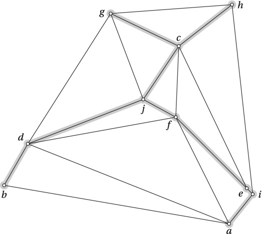
Figure 7-3. A Euclidean graph and its minimum spanning tree (highlighted)
As it turns out, it is. Consider any spanning tree without the minimum-weight edge (e,i). The spanning tree would have to include both e and i (by definition), so it would also include a single path from e to i. If we now were to add (e,i) to the mix, we’d get a cycle, and in order to get back to a proper spanning tree, we’d have to remove one of the edges of this cycle—it doesn’t matter which. Because (e,i) is the smallest, removing any other edge would yield a smaller tree than we started out with. Right? In other words, any tree not including the shortest edge can be made smaller, so the minimum spanning tree must include the shortest edge. (As you’ll see, this is the basic idea behind Kruskal’s algorithm.)
What if we consider all the edges incident at a single node—can we draw any conclusions then? Take a look at b, for example. By the definition of spanning trees, we must connect b to the rest somehow, which means we must include either (b,d) or (b,a). Again, it seems tempting to choose the shortest of the two. And once again, the greedy choice turns out to be very sensible. Once again, we prove that the alternative is inferior using a proof by contradiction: Assume that it was better to use (b,a). We’d build our minimum spanning tree with (b,a) included. Then, just for fun, we’d add (b,d), creating a cycle. But, hey—if we remove (b,a), we have another spanning tree, and because we’ve switched one edge for a shorter one, this new tree must be smaller. In other words, we have a contradiction, and the one without (b,d) couldn’t have been minimal in the first place. And this is the basic idea behind Prim’s algorithm, which we’ll look at after Kruskal’s.
In fact, both of these ideas are special cases of a more general principle involving cuts. A cut is simply a partitioning of the graph nodes into two sets, and in this context we’re interested in the edges that pass between these two node sets. We say that these edges cross the cut. For example, imagine drawing a vertical line in Figure 7-3, right between d and g; this would give a cut that is crossed by five edges. By now I’m sure you’re catching on: We can be certain that it will be safe to include the shortest edge across the cut, in this case (d,j). The argument is once again exactly the same: We build an alternative tree, which will necessarily include at least one other edge across the cut (in order to keep the graph connected). If we then add (d,j), at least one of the other, longer edges across the cut would be part of the same cycle as (d,j), meaning that it would be safe to remove the other edge, giving a smaller spanning tree.
You can see how the two first ideas are special cases of this “shortest edge across a cut” principle: Choosing the shortest edge in the graph will be safe because it will be shortest in every cut in which it participates, and choosing the shortest edge incident to any node will be safe because it’s the shortest edge over the cut that separates that node from the rest of the graph. In the following, I expand on these ideas, turning them into two full-fledged greedy algorithms for finding minimum spanning trees. The first (Kruskal’s) is close to the prototypical greedy algorithm, while the next (Prim’s) uses the principles of traversal, with the greedy choice added on top.
What About the Rest?
Showing that the first greedy choice is OK isn’t enough. We need to show that the remaining problem is a smaller instance of the same problem—that our reduction is safe to use inductively. In other words, we need to establish optimal substructure. This isn’t too hard (Exercise 7-12), but there’s another approach that’s perhaps even simpler here: We prove the invariant that our solution is part (a subgraph) of a minimum spanning tree. We keep adding edges as long as the solution isn’t a spanning tree (that is, as long as there are edges left that won’t form a cycle), so if this invariant is true, the algorithm must terminate with a full, minimum spanning tree.
So, is the invariant true? Initially, our partial solution is empty, which is clearly a partial, minimum spanning tree. Now, assume inductively that we’ve built some partial, minimum spanning tree T and that we add a safe edge (that is, one that doesn’t create a cycle and that is the shortest one across some cut). Clearly, the new structure is still a forest (because we meticulously avoid creating cycles). Also, the reasoning in the previous section still applies: Among the spanning trees containing T, the one(s) including this safe edge will be smaller than those that don’t. Because (by assumption), at least one of the trees containing T is a minimum spanning tree, at least one of those containing T and the safe edge will also be a minimum spanning tree.
Kruskal’s Algorithm
This algorithm is close to the general greedy approach outlined at the beginning of this chapter: Sort the edges and start picking. Because we’re looking for short edges, we sort them by increasing length (or weight). The only wrinkle is how to detect edges that would lead to an invalid solution. The only way to invalidate our solution would be to add a cycle, but how can we check for that? A straightforward solution would be to use traversal; every time we consider an edge (u,v), we traverse our tree from u to see whether there is a path to v. If there is, we discard it. This seems a bit wasteful, though; in the worst case, the traversal check would take linear time in the size of our partial solution.
What else could we do? We could maintain a set of the nodes in our tree so far, and then for a prospective edge (u,v), we’d see whether both were in the solution. This would mean that sorting the edges is what dominates; checking each edge could be done in constant time. There’s just one crucial flaw in this plan: It won’t work. It would work if we could guarantee that the partial solution was connected at every step (which is what we’ll be doing in Prim’s algorithm), but we can’t. So even if two nodes are part of our solution so far, they may be in different trees, and connecting them would be perfectly valid. What we need to know is that they aren’t in the same tree.
Let’s try to solve this by making each node in the solution know which component (tree) it belongs to. We can let one of the nodes in a component act as a representative, and then all the nodes in that component could point to that representative. This leaves the problem of combining components. If all nodes of the merged component had to point to the same representative, this combination (or union) would be a linear operation. Can we do better? We could try; for example, we could let each node point to some other node, and we’d follow that chain until we reached the representative (which would point to itself). Joining would then just be a matter of having one representative point to the other (constant time). There are no immediate guarantees on how long the chain of references would be, but it’s a first step, at least.
This is what I’ve done in Listing 7-3, using the map C to implement the “pointing.” As you can see, each node is initially the representative of its own component, and then I repeatedly connect components with new edges, in sorted order. Note that the way I’ve implemented this, I’m expecting an undirected graph where each edge is represented just once (that is, using one of its directions, chosen arbitrarily).11 As always, I’m assuming that every node is a key in the graph, though, possibly with an empty weight map (that is, G[u] = {} if u has no out-edges).
Listing 7-3. A Naïve Implementation of Kruskal’s Algorithm
def naive_find(C, u):                           # Find component rep.
    while C[u] != u:                            # Rep. would point to itself
        u = C[u]
    return u

def naive_union(C, u, v):
    u = naive_find(C, u)                        # Find both reps
    v = naive_find(C, v)
    C[u] = v                                    # Make one refer to the other

def naive_kruskal(G):
    E = [(G[u][v],u,v) for u in G for v in G[u]]
    T = set()                                   # Empty partial solution
    C = {u:u for u in G}                        # Component reps
    for _, u, v in sorted(E):                   # Edges, sorted by weight
        if naive_find(C, u) != naive_find(C, v):
            T.add((u, v))                       # Different reps? Use it!
            naive_union(C, u, v)                # Combine components
    return T
The naïve Kruskal works, but it’s not all that great. (What, the name gave it away?) In the worst case, the chain of references we need to follow in naive_find could be linear. A rather obvious idea might be to always have the smaller of the two components in naive_union point to the larger, giving us some balance. Or we could think even more in terms of a balanced tree and give each node a rank, or height. If we always made the lowest-ranking representative point to the highest-ranking one, we’d get a total running time of O(m lg n) for the calls to naive_find and naive_union (see Exercise 7-16).
This would actually be fine because the sorting operation to begin with is Θ(m lg n) anyway.12 There is one other trick that is commonly used in this algorithm, though, called path compression. It entails “pulling the pointers along” when doing a find, making sure all the nodes we examine on our way now point directly to the representative. The more nodes point directly at the representative, the faster things should go in later finds, right? Sadly, the reasoning behind exactly how and why this helps is far too knotty for me to go into here (although I’d recommend Sect. 21.4 in Introduction to Algorithms by Cormen et al., if you’re interested). The end result, though, is that the worst-case total running time of the unions and finds is O(mα(n)), where α(n) is almost a constant. In fact, you can assume that α(n) ≤ 4, for any even remotely plausible value for n. For an improved implementation of find and union, see Listing 7-4.
Listing 7-4. Kruskal’s Algorithm
def find(C, u):
    if C[u] != u:
        C[u] = find(C, C[u])                    # Path compression
    return C[u]

def union(C, R, u, v):a
    u, v = find(C, u), find(C, v)
    if R[u] > R[v]:                             # Union by rank
        C[v] = u
    else:
        C[u] = v
    if R[u] == R[v]:                            # A tie: Move v up a level
        R[v] += 1

def kruskal(G):
    E = [(G[u][v],u,v) for u in G for v in G[u]]
    T = set()
    C, R = {u:u for u in G}, {u:0 for u in G}   # Comp. reps and ranks
    for _, u, v in sorted(E):
        if find(C, u) != find(C, v):
            T.add((u, v))
            union(C, R, u, v)
    return T
All in all, the running time of Kruskal’s algorithm is Θ(m lg n), which comes from the sorting.
Note that you might want to represent your spanning trees differently (that is, not as sets of edges). The algorithm should be easy to modify in this respect—or you could just build the structure you want based on the edge set T.
Note The subproblem structure used in Kruskal’s algorithm is an example of a matroid, where the feasible partial solutions are simply sets—in this case, cycle-free edge sets. For matroids, greed works. Here are the rules: All subsets of feasible sets must also be feasible, and larger sets must have elements that can extend smaller ones.
Prim’s Algorithm
Kruskal’s algorithm is simple on the conceptual level—it’s a direct translation of the greedy approach to the spanning tree problem. As you just saw, though, there is some complexity in the validity checking. In this respect, Prim’s algorithm is a bit simpler.13 The main idea in Prim’s algorithm is to traverse the graph from a starting node, always adding the shortest edge connected to the tree. This is safe because the edge will be the shortest one crossing the cut around our partial solution, as explained earlier.
This means that Prim’s algorithm is just another traversal algorithm, which should be a familiar concept if you’ve read Chapter 5. As discussed in that chapter, the main difference between traversal algorithms is the ordering of our “to-do” list—among the unvisited nodes we’ve discovered, which one do we grow our traversal tree to next? In breadth-first search, we used a simple queue (that is, a deque); in Prim’s algorithm, we simply replace this queue with a priority queue, implemented with a heap, using the heapq library (discussed in a “Black Box” sidebar in Chapter 6).
There is one important issue here, though: Most likely, we will discover new edges pointing to nodes that are already in our queue. If the new edge we discovered was shorter than the previous one, we should adjust the priority based on this new edge. This, however, can be quite a hassle. We’d need to find the given node inside the heap, change the priority, and then restructure the heap so that it would still be correct. You could do that by having a mapping from each node to its position in the heap, but then you’d have to update that mapping when performing heap operations, and you could no longer use the heapq library.
It turns out there’s another way, though. A really pretty solution, which will also work with other priority-based traversals (such as Dijkstra’s algorithm and A*, discussed in Chapter 9), is to simply add the nodes multiple times. Each time you find an edge to a node, you add the node to the heap (or other priority queue) with the appropriate weight, and you don’t care if it’s already in there. Why could this possibly work?
- We’re using a priority queue, so if a node has been added multiple times, by the time we remove one of its entries, it will be the one with the lowest weight (at that time), which is the one we want.
- We make sure we don’t add the same node to our traversal tree more than once. This can be ensured by a constant-time membership check. Therefore, all but one of the queue entries for any given node will be discarded.
- The multiple additions won’t affect asymptotic running time (see Exercise 7-17).
There are important consequences for the actual running time as well. The (much) simpler code isn’t only easier to understand and maintain; it also has a lot less overhead. And because we can use the super-fast heapq library, the net consequence is most likely a large performance gain. (If you’d like to try the more complex version, which is used in many algorithm books, you’re welcome, of course.)
Note Re-adding a node with a lower weight is equivalent to a relaxation, as discussed in Chapter 4. As you’ll see, I also add the predecessor node to the queue, making any explicit relaxation unnecessary. When implementing Dijkstra’s algorithm in Chapter 9, however, I use a separate relax function. These two approaches are interchangeable (so you could have Prim’s with relax and Dijkstra’s without it).
You can see my version of Prim’s algorithm in Listing 7-5. Because heapq doesn’t (yet) support sorting keys, as list.sort and friends do, I’m using (weight, node) pairs in the heap, discarding the weights when the nodes are popped off. Beyond the use of a heap, the code is similar to the implementation of breadth-first search in Listing 5-10. That means that a lot of the understanding here should come for free.
Listing 7-5. Prim’s Algorithm
from heapq import heappop, heappush

def prim(G, s):
    P, Q = {}, [(0, None, s)]
    while Q:
        _, p, u = heappop(Q)
        if u in P: continue
        P[u] = p
        for v, w in G[u].items():
            heappush(Q, (w, u, v))
    return P
Note that unlike kruskal, in Listing 7-4, the prim function in Listing 7-5 assumes that the graph G is an undirected graph where both directions are explicitly represented, so we can easily traverse each edge in both directions.14
As with Kruskal’s algorithm, you may want to represent the resulting spanning tree differently from what I do here. Rewriting that part should be pretty easy.
Note The subproblem structure used in Prim’s algorithm is an example of a greedoid, which is a simplification and generalization of matroids where we no longer require all subsets of feasible sets to be feasible. Sadly, having a greedoid is not in itself a guarantee that greed will work—though it is a step in the right direction.
A SLIGHTLY DIFFERENT PERSPECTIVE
In their historical overview of minimum spanning tree algorithms, Ronald L. Graham and Pavol Hell outline three algorithms that they consider especially important and that have played a central role in the history of the problem. The first two are the algorithms that are commonly attributed to Kruskal and Prim (although the second one was originally formulated by Vojtěch Jarník in 1930), while the third is the one initially described by Boru˚vka. Graham and Hell succinctly explain the algorithms as follows. A partial solution is a spanning forest, consisting of a set of fragments (components, trees). Initially, each node is a fragment. In each iteration, edges are added, joining fragments, until we have a spanning tree.
Algorithm 1: Add a shortest edge that joins two different fragments.
Algorithm 2: Add a shortest edge that joins the fragment containing the root to another fragment.
Algorithm 3: For every fragment, add the shortest edge that joins it to another fragment.
For algorithm 2, the root is chosen arbitrarily at the beginning. For algorithm 3, it is assumed that all edge weights are different to ensure that no cycles can occur. As you can see, all three algorithms are based on the same fundamental fact—that the shortest edge over a cut is safe. Also, in order to implement them efficiently, you need to be able to find shortest edges, detect whether two nodes belong to the same fragment, and so forth (as explained for algorithms 1 and 2 in the main text). Still, these brief explanations can be useful as a memory aid or to get the bird’s-eye perspective on what’s going on.
Greed Works. But When?
Although induction is generally used to show that a greedy algorithm is correct, there are some extra “tricks” that can be employed. I’ve already used some in this chapter, but here I’ll try to give you an overview, using some simple problems involving time intervals. It turns out there are many problems of this type that can be solved by greedy algorithms. I’m not including code for these; the implementations are pretty straightforward (although it might be a useful exercise to actually implement them).
Keeping Up with the Best
This is what Kleinberg and Tardos (in Algorithm Design) call staying ahead. The idea is to show that as you build your solution, one step at a time, the greedy algorithm will always have gotten at least as far as a hypothetical optimal algorithm would have. Once you reach the finish line, you’ve shown that greed is optimal. This technique can be useful in solving a common example of greed: resource scheduling.
The problem involves selecting a set of compatible intervals. Normally, we think of these intervals as time intervals (see Figure 7-4). Compatibility simply means that none of them should overlap, so this could be used to model requests for using a resource, such as a lecture hall, for certain time periods. Another example would be to let you be the “resource” and to let the intervals be various activities you’d like to participate in. Either way, our optimization task is to choose as many mutually compatible (nonoverlapping) intervals as possible. For simplicity, we can assume that no start or end points are identical. Handling identical values is not significantly harder.
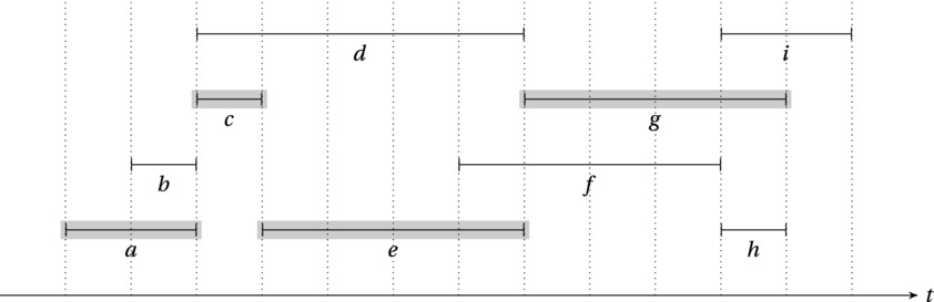
Figure 7-4. A set of random intervals where at most four mutually compatible intervals (for example, a, c, e and g) can be found
There are two obvious candidates for greedy selection here: If we go from left to right on the timeline, we might want to start with either the interval that starts first or the one that ends first, eliminating any other overlapping intervals. I hope it is clear that the first alternative can’t work (Exercise 7-18), which leaves us to show that the other one does work.
The algorithm is (roughly) as follows:
- Include the interval with the lowest finish time in the solution.
- Remove all of the remaining intervals that overlap with the one from step 1.
- Any remaining intervals? Go to step 1.
Running this algorithm on the interval set in Figure 7-4 results in the highlighted set of intervals (a, c, e and g). The resulting solution is clearly valid; that is, there aren’t any overlapping intervals in it. This will be the case in general; we need show only that it’s optimal, that is, that we have as many intervals as possible. Let’s try to apply the idea of staying ahead.
Let’s say our intervals are, in the order in which they were added, i1 … ik, and that the hypothetical, optimal solution gives the intervals j1 … jm. We want to show that k = m. Assume that the optimal intervals are sorted by finishing (and starting) times.15 To show that our algorithm stays ahead of the optimal one, we need to show that for any r ≤ k, the finish time of ir is at least as early as that of jr, and we can prove this by induction.
For r = 1, it is obviously correct: The greedy algorithm chooses i1, which is the element with the minimum finish time. Now, let r > 1 and assume that our hypothesis holds for r - 1. The question then becomes whether it is possible for the greedy algorithm to “fall behind” at this step. That is, is it possible that the finish time for ir could now be greater than that of jr? The answer is clearly no, because the greedy algorithm could just as well have chosen jr (which is compatible with jr-1, and therefore also with ir-1, which finishes at least as early).
So, the greedy algorithm keeps up with the best, all the way to the end. However, this “keeping up” dealt only with finishing times, not the number of intervals. We need to show that keeping up will yield an optimal solution, and we can do so by contradiction: If the greedy algorithm is not optimal, then m > k. For every r, including r = k, we know that ir finishes at least as early as jr. Because m > k, there must be an interval jr+1 that we didn’t use. This must start after jr, and therefore after ir, which means that we could have—and, indeed, would have—included it. In other words, we have a contradiction.
No Worse Than Perfect
This is a technique I used in showing the greedy choice property for Huffman’s algorithm. It involves showing that you can transform a hypothetical optimal solution to the greedy one, without reducing the quality. Kleinberg and Tardos call this an exchange argument. Let’s put a twist on the interval problem. Instead of having fixed starting and ending times, we now have a duration and a deadline, and you’re free to schedule the intervals—let’s call them tasks—as you want, as long as they don’t overlap. You also have a given starting time, of course.
However, any task that goes past its deadline incurs a penalty equal to its delay, and you want to minimize the maximum of these delays. On the surface, this might seem like a rather complex scheduling problem (and, indeed, many scheduling problems are really hard to solve). Surprisingly, though, you can find the optimum schedule through a super-simple greedy strategy: Always perform the most urgent task. As is often the case for greedy algorithms, the correctness proof is a bit tougher than the algorithm itself.
The greedy solution has no gaps in it. As soon as we’re done with one task, we start the next. There will also be at least one optimal solution without gaps—if we have an optimal solution with gaps, we can always close these up, resulting in earlier finish times for the later tasks. Also, the greedy solution will have no inversions (jobs scheduled before other jobs with earlier deadlines). We can show that all solutions without gaps or inversions have the same maximum delay. Two such solutions can differ only in the order of tasks with identical deadlines, and these must be scheduled consecutively. Among the tasks in such a consecutive block, the maximum delay depends only on the last task, and this delay doesn’t depend on the order of the tasks.
The only thing that remains to be proven is that there exists an optimal solution without gaps or inversions, because it would be equivalent to the greedy solution. This proof has three parts:
- If the optimal solution has an inversion, there are two consecutive tasks where the first has a later deadline than the second.
- Switching these two removes one inversion.
- Removing this inversion will not increase the maximum delay.
The first point should be obvious enough. Between two inverted tasks, there must be some point where the deadlines start decreasing, giving us the two consecutive, inverted tasks. As for the second point, swapping the tasks clearly removes one inversion, and no new inversions are created. The third point requires a little care. Swapping tasks i and j (so j now comes first) can potentially increase the lateness of only i; all other tasks are safe. In the new schedule, i finishes where j finished before. Because (by assumption) the deadline of i was later than that of j, the delay cannot possibly have increased. Thus, the third part of the proof is done.
It should be clear that these parts together show that the greedy schedule minimizes the maximum delay.
Staying Safe
This is where we started: To make sure a greedy algorithm is correct, we must make sure each greedy step along the way is safe. One way of doing this is the two-part approach of showing (1) the greedy choice property, that is, that a greedy choice is compatible with optimality, and (2) optimal substructure, that is, that the remaining subproblem is a smaller instance that must also be solved optimally. The greedy choice property, for example, can be shown using an exchange argument (as was done for the Huffman algorithm).
Another possibility is to treat safety as an invariant. Or, in the words of Michael Soltys (see the “References” section of Chapter 4), we need to show that if we have a promising partial solution, a greedy choice will yield a new, bigger solution that is also promising. A partial solution is promising if it can be extended to an optimal solution. This is the approach I took in the section “What about the rest?” earlier in this chapter; there, a solution was promising if it was contained in (and, thus, could be extended to) a minimum spanning tree. Showing that “the current partial solution is promising” is an invariant of the greedy algorithm, as you keep making greedy choices, is really all you need.
Let’s consider a final problem involving time intervals. The problem is simple enough, and so is the algorithm, but the correctness proof is rather involved.16 It can serve as an example of the effort that may be required to show that a relatively simple greedy algorithm is correct.
This time, we once again have a set of tasks with deadlines, as well as a starting time (such as the present). This time, though, these are hard deadlines—if we can’t get a task done before its deadline, we can’t take it on at all. In addition, each task has a given profit associated with it. As before, we can perform only one task at a time, and we can’t split them into pieces, so we’re looking for a set of jobs that we can actually do, and that gives us as large a total profit as possible. However, to keep things simple, this time all tasks take the same amount of time—one time step. If d is the latest deadline, as measured in time steps from the starting point, we can start with an empty schedule of d empty slots and then fill those slots with tasks.
The solution to this problem is, in a way, doubly greedy. First, we consider the tasks by decreasing profit, starting with the most profitable task; that’s the first greedy part. Then comes the second part: We place each task in the latest possible free slot that it can occupy, based on its deadline. If there is no free, valid slot, we discard the task. Once we’re done, if we haven’t filled all the slots, we’re certainly free to perform tasks earlier, so as to remove the gaps—it won’t affect the profit or allow us to perform any more tasks. To get a feel for this solution, you might want to actually implement it (Exercise 7-20).
The solution sounds intuitively appealing; we give the profitable tasks precedence, and we make sure they use a minimum of our precious “early time,” by pushing them as far toward their deadline as possible. But, once again, we won’t rely on intuition. We’ll use a bit of induction, showing that as we add tasks in this greedy fashion, our schedule stays promising.
Caution The following presentation does not involve any deep math or rocket science and is more of an informal explanation than a full, technical proof. Still, it is a bit involved and might hurt your brain. If you don’t feel up to it, feel free to skip ahead to the chapter summary.
As is invariably the case, the initial, empty solution is promising. In moving beyond the base case, it’s important to remember that the schedule is really promising only if it can be extended to an optimal schedule using the remaining tasks, as this is the only way we’re allowed to extend it. Now, assume we have a promising partial schedule P. Some of its slots are filled in, and some are not. The fact that P is promising means that it can be extended to an optimal schedule—let’s call it S. Also, let’s say T is the next task under consideration.
We now have four cases to consider:
- T won’t fit in P, because there is no room before the deadline. In this case, T can’t affect anything, so P is still promising once T is discarded.
- T will fit in P, and it ends up in the same position as in S. In this case, we’re actually extending toward S, so P is still promising.
- T will fit, but it ends up somewhere else. This might seem somewhat troubling.
- T will fit, but S doesn’t contain it. Even more troubling, perhaps.
Clearly we need to address the last two cases, because they seem to be building away from the optimal schedule S. The thing is, there may be more than one optimal schedule—we just need to show that we can still reach one of them after T has been added.
First, let’s consider the case where we greedily add T, and it’s not in the same place as it would have been in S. Then we can build a schedule that’s almost like S, except that T has swapped places with another task T’. Let’s call this other schedule S’. By construction, T is placed as late as possible in S’, which means it must be placed earlier in S. Conversely, T’ must be placed later in S and therefore earlier in S’. This means that we cannot have broken the deadline of T’ when constructing S’, so it’s a valid solution. Also, because S and S’ consist of the same tasks, the profits must be identical.
The only case that remains is if T is not scheduled in the optimal schedule S. Again, let S’ be almost like S. The only difference is that we’ve scheduled T with our algorithm, effectively “overwriting” some other task T’ in S. We haven’t broken any deadlines, so S’ is valid. We also know that we can get from P to S’ (by almost following the steps needed to get to S, just using T instead of T’).
The last question then becomes, does S’ have the same profit as S? We can prove that it does, by contradiction. Assume that T’ has a greater profit than T, which is the only way in which S could have a higher profit. If this were the case, the greedy algorithm would have considered T’ before T. As there is at least one free slot before the deadline of T’, the greedy algorithm would have scheduled it, necessarily in a different position than T, and therefore in a different position than in S. But we assumed that we could extend P to S, and if it has a task in a different position, we have a contradiction.
Note This is an example of a proof technique called proof by cases, where we add some conditions to the situation and make sure to prove what we want for all cases that these conditions can create.
Summary
Greedy algorithms are characterized by how they make decisions. In building a solution, step-by-step, each added element is the one that looks best at the moment it’s added, without concern for what went before or what will happen later. Such algorithms can often be quite simple to design and implement, but showing that they are correct (that is, optimal) is often challenging. In general, you need to show that making a greedy choice is safe—that if the solution you had was promising, that is, it could be extended to an optimal one, then the one after the greedy choice is also promising. The general principles, as always, is that of induction, though there are a couple of more specialized ideas that can be useful. For example, if you can show that a hypothetical optimal solution can be modified to become the greedy solution without loss of quality, then the greedy solution is optimal. Or, if you can show that during the solution building process, the greedy partial solutions in some sense keep up with a hypothetical optimal sequence of solutions, all the way to the final solution, you can (with a little care) use that to show optimality.
Important greedy problems and algorithms discussed in this chapter include the knapsack problem (selecting a weight-bounded subset of items with maximum value), where the fractional version can be solved greedily; Huffman trees, which can be used to create optimal prefix codes and are built greedily by combining the smallest trees in the partial solution; and minimum spanning trees, which can be built using Kruskal’s algorithm (keep adding the smallest valid edge) or Prim’s algorithm (keep connecting the node that is closest to your tree).
If You’re Curious …
There is a deep theory about greedy algorithms that I haven’t really touched upon in this chapter, dealing with such beasts as matroids, greedoids, and so-called matroid embeddings. Although the greedoid stuff is a bit hard and the matroid embedding stuff can get really confusing fast, matroids aren’t really that complicated, and they present an elegant perspective on some greedy problems. (Greedoids are more general, and matroid embeddings are the most general of the three, actually covering all greedy problems.) For more information on matroids, you could have a look at the book by Cormen et al. (see the “References” section of Chapter 1).
If you’re interested in why the change-making problem is hard in general, you should have a look at the material in Chapter 11. As noted earlier, though, for a lot of currency systems, the greedy algorithm works just fine. David Pearson has designed an algorithm for checking whether this is the case, for any given currency; if you’re interested, you should have a look at his paper (see “References”).
If you find you need to build minimum directed spanning trees, branching out from some starting node, you can’t use Prim’s algorithm. A discussion of an algorithm that will work for finding these so-called min-cost arborescences can be found in the book by Kleinberg and Tardos (see the “References” section of Chapter 1).
Exercises
7-1. Give an example of a set of denominations that will break the greedy algorithm for giving change.
7-2. Assume that you have coins whose denominations are powers of some integer k > 1. Why can you be certain that the greedy algorithm for making change would work in this case?
7-3. If the weights in some selection problem are unique powers of two, a greedy algorithm will generally maximize the weight sum. Why?
7-4. In the stable marriage problem, we say that a marriage between two people, say, Jack and Jill, is feasible if there exists a stable pairing where Jack and Jill are married. Show that the Gale-Shapley algorithm will match each man with his highest-ranking feasible wife.
7-5. Jill is Jack’s best feasible wife. Show that Jack is Jill’s worst feasible husband.
7-6. Let’s say the various things you want to pack into your knapsack are partly divisible. That is, you can divide them at certain evenly spaced points (such as a candy bar divided into squares). The different items have different spacings between their breaking points. Could a greedy algorithm still work?
7-7. Show that the codes you get from a Huffman code are free of ambiguity. That is, when decoding a Huffman-coded text, you can always be certain of where the symbol boundaries go and which symbols go where.
7-8. In the proof for the greedy choice property of Huffman trees, it was assumed that the frequencies of a and d were different. What happens if they’re not?
7-9. Show that a bad merging schedule can give a worse running time, asymptotically, than a good one and that this really depends on the frequencies.
7-10. Under what circumstances can a (connected) graph have multiple minimum spanning trees?
7-11. How would you build a maximum spanning tree (that is, one with maximum edge-weight sum)?
7-12. Show that the minimum spanning tree problem has optimal substructure.
7-13. What will Kruskal’s algorithm find if the graph isn’t connected? How could you modify Prim’s algorithm to do the same?
7-14. What happens if you run Prim’s algorithm on a directed graph?
7-15. For n points in the plane, no algorithm can find a minimum spanning tree (using Euclidean distance) faster than loglinear in the worst case. How come?
7-16. Show that m calls to either union or find would have a running time of O(m lg n) if you used union by rank.
7-17. Show that when using a binary heap as priority queue during a traversal, adding nodes once for each time they’re encountered won’t affect the asymptotic running time.
7-18. In selecting the largest nonoverlapping subset of a set of intervals, going left to right, why can’t we use a greedy algorithm based on starting times?
7-19. What would the running time be of the algorithm finding the largest set of nonoverlapping intervals?
7-20. Implement the greedy solution for the scheduling problem where each task has a cost and a hard deadline and where all tasks take the same amount of time to perform.
References
Gale, D. and Shapley, L. S. (1962). College admissions and the stability of marriage. The American Mathematical Monthly, 69(1):9-15.
Graham, R. L. and Hell, P. (1985). On the history of the minimum spanning tree problem. IEEE Annals on the History of Computing, 7(1).
Gusfield, D. and Irving, R. W. (1989). The Stable Marriage Problem: Structure and Algorithms. The MIT Press.
Helman, P., Moret, B. M. E., and Shapiro, H. D. (1993). An exact characterization of greedy structures. SIAM Journal on Discrete Mathematics, 6(2):274-283.
Knuth, D. E. (1996). Stable Marriage and Its Relation to Other Combinatorial Problems: An Introduction to the Mathematical Analysis of Algorithms. American Mathematical Society.
Korte, B. H., Lovász, L., and Schrader, R. (1991). Greedoids. Springer-Verlag.
Nešetřil, J., Milková, E., and Nešetřilová, H. (2001). Otakar Borůvka on minimum spanning tree problem: Translation of both the 1926 papers, comments, history. Discrete Mathematics, 233(1-3):3-36.
Pearson, D. (2005). A polynomial-time algorithm for the change-making problem. Operations Research Letters, 33(3):231-234.
___________________________
1No, it’s not to run away and buy comic books.
2The idea for this version of the problem comes from Michael Soltys (see references in Chapter 4).
3To be on the safe side, just let me emphasize that this greedy solution would not work in general, with an arbitrary set of weights. The distinct powers of two are key here.
4If we view each object individually, this is often called 0-1 knapsack because we can take 0 or 1 of each object.
5Not only is it unimportant whether zero means left or right, it is also unimportant which subtrees are on the left and which are on the right. Shuffling them won’t matter to the optimality of the solution.
6If a future version of the heapq library lets you use a key function, such as in list.sort, you’d no longer need this tuple wrapping at all, of course.
7They might also have equal weights/frequencies; that doesn’t affect the argument.
8By the way, did you know that the ZIP code of Huffman, Texas, is 77336?
9You can, in fact, combine Borůvka’s algorithm with Prim’s to get a faster algorithm.
10Do you see why the result cannot contain any cycles, as long as we assume positive edge weights?
11Going back and forth between this representation and one where you have edges both ways isn’t really hard, but I’ll leave the details as an exercise for the reader.
12We’re sorting m edges, but we also know that m is O(n2), and (because the graph is connected), m is Ω(n). Because Θ(lg n2) = Θ(2.lg n) = Θ(lg n), we get the result.
13Actually, the difference is deceptive. Prim’s algorithm is based on traversal and heaps—concepts we’ve already dealt with—while Kruskal’s algorithm introduced a new disjoint set mechanism. In other words, the difference in simplicity is mostly a matter of perspective and abstraction.
14As I mentioned when discussing Kruskal’s algorithm, adding and removing such redundant reverse edges is quite easy, if you need to do so.
15Because the intervals don’t overlap, sorting by starting and finishing times is equivalent.
16Versions of this problem can be found in Soltys’ book (see “References” in Chapter 4) and that of Cormen et al. (see “References” in Chapter 1). My proof closely follows Soltys’s, while Cormen et al. choose to prove that the problem forms a matroid, which means that a greedy algorithm will work on it.