Table of Contents for
Python Algorithms: Mastering Basic Algorithms in the Python Language, Second Edition
 Python Algorithms: Mastering Basic Algorithms in the Python Language, Second Edition
Published by
Apress, 2015
Python Algorithms: Mastering Basic Algorithms in the Python Language, Second Edition
Published by
Apress, 2015
- Cover
- Title
- Copyright
- Dedication
- Contents at a Glance
- Contents
- About the Author
- About the Technical Reviewer
- Acknowledgments
- Preface
- Chapter 1: Introduction
- Chapter 2: The Basics
- Chapter 3: Counting 101
- Chapter 4: Induction and Recursion … and Reduction
- Chapter 5: Traversal: The Skeleton Key of Algorithmics
- Chapter 6: Divide, Combine, and Conquer
- Chapter 7: Greed Is Good? Prove It!
- Chapter 8: Tangled Dependencies and Memoization
- Chapter 9: From A to B with Edsger and Friends
- Chapter 10: Matchings, Cuts, and Flows
- Chapter 11: Hard Problems and (Limited) Sloppiness
- Appendix A: Pedal to the Metal: Accelerating Python
- Appendix B: List of Problems and Algorithms
- Appendix C: Graph Terminology
- Appendix D: Hints for Exercises
- Index

Traversal: The Skeleton Key of Algorithmics
You are in a narrow hallway. This continues for several metres and ends in a doorway. Halfway along the passage you can see an archway where some steps lead downwards. Will you go forwards to the door (turn to 5), or creep down the steps (turn to 344)?
— Steve Jackson, Citadel of Chaos
Graphs are a powerful mental (and mathematical) model of structure in general; if you can formulate a problem as one dealing with graphs, even if it doesn’t look like a graph problem, you are probably one step closer to solving it. It just so happens that there is a highly useful mental model for graph algorithms as well—a skeleton key, if you will.1 That skeleton key is traversal: discovering, and later visiting, all the nodes in a graph. And it’s not just about obvious graphs. Consider, for example, how painting applications such as GIMP or Adobe Photoshop can fill a region with a single color, so-called flood fill. That’s an application of what you’ll learn here (see Exercise 5-4). Or perhaps you want to serialize some complex data structure and need to make sure you examine all its constituent objects? That’s traversal. Listing all files and directories in a part of the file system? Manage dependencies between software packages? More traversal.
But traversal isn’t only useful directly; it’s a crucial component and underlying principle in many other algorithms, such as those in Chapters 9 and 10. For example, in Chapter 10, we’ll try to match n people with n jobs, where each person has skills that match only some of the jobs. The algorithm works by tentatively assigning people to jobs but then reassigning them if someone else needs to take over. This reassignment can then trigger another reassignment, possibly resulting in a cascade. As you’ll see, this cascade involves moving back and forth between people and jobs, in a sort of zig-zag pattern, starting with an idle person and ending with an available job. What’s going on here? You guessed it: traversal.
I’ll cover the idea from several angles and, in several versions, trying to tie the various strands together where possible. This means covering two of the most well-known basic traversal strategies, depth-first search and breadth-first search, building up to a slightly more complex traversal-based algorithm for finding so-called strongly connected components.
Traversal is useful in that it lets us build a layer abstraction on top of some basic induction. Consider the problem of finding the connected components of a graph (see Figure 5-1 for an example). As you may recall from Chapter 2, a graph is connected if there is a path from each node to each of the others and if the connected components are the maximal subgraphs that are (individually) connected. One way of finding a connected component would be to start at some place in the graph and gradually grow a larger connected subgraph until we can’t get any further. How can we be sure that we have then reconstructed an entire component?
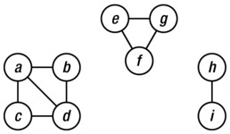
Figure 5-1. An undirected graph with three connected components
Let’s look at the following related problem. Show that you can order the nodes in a connected graph, v1, v2, . . . , vn, so that for any i = 1 . . . n, the subgraph over v1, . . . , vi is connected. If we can show this and we can figure out how to do the ordering, we can go through all the nodes in a connected component and know when they’re all used up.
How do we do this? Thinking inductively, we need to get from i–1 to i. We know that the subgraph over the i–1 first nodes is connected. What next? Well, because there are paths between any pair of nodes, consider a node u in the first i–1 nodes and a node v in the remainder. On the path from u to v, consider the last node that is in the component we’ve built so far, as well as the first node outside it. Let’s call them x and y. Clearly there must be an edge between them, so adding y to the nodes of our growing component keeps it connected, and we’ve shown what we set out to show.
I hope you can see how easy the resulting procedure actually is. It’s just a matter of adding nodes that are connected to the component, and we discover such nodes by following an edge. An interesting point is that as long as we keep connecting new nodes to our component in this way, we’re building a tree. This tree is called a traversal tree and is a spanning tree of the component we’re traversing. (For a directed graph, it would span only the nodes we could reach, of course.)
To implement this procedure, we need to keep track of these “fringe” or “frontier” nodes that are just one edge away. If we start with a single node, the frontier will simply be its neighbors. As we start exploring, the neighbors of newly visited nodes will form the new fringe, while those nodes we visit now fall inside it. In other words, we need to maintain the fringe as a collection of some sort, where we can remove the nodes we visit and add their neighbors, unless they’re already on the list or we’ve already visited them. It becomes a sort of to-do list of nodes we want to visit but haven’t gotten around to yet. You can think of the ones we have visited as being checked off.
For those of you who have played old-school role-playing games such as Dungeons & Dragons (or, indeed, many of today’s video games), Figure 5-2 might help clarify these ideas. It shows a typical dungeon map.2 Think of the rooms (and corridors) as nodes and the doors between them as edges. There are some multiple edges (doors) here, but that’s really not a problem. I’ve also added a “you are here” marker to the map, along with some tracks indicating how you got there.
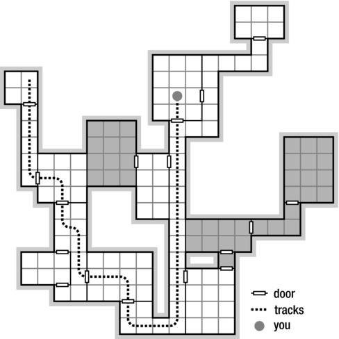
Figure 5-2. A partial traversal of a typical role-playing dungeon. Think of the rooms as nodes and the doors as edges. The traversal tree is defined by your tracks; the fringe (the traversal queue) consists of the neighboring rooms, the light ones without footprints. The remaining (darkened) rooms haven’t been discovered yet
Notice that there are three kinds of rooms: the ones you’ve actually visited (those with tracks through them), those you know about because you’ve seen their doors, and those you don’t know about yet (darkened). The unknown rooms are (of course) separated from the visited rooms by a frontier of known but unvisited rooms, just like in any kind of traversal. Listing 5-1 gives a simple implementation of this general traversal strategy (with the comments referring to graphs rather than dungeons).3
Listing 5-1. Walking Through a Connected Component of a Graph Represented Using Adjacency Sets
def walk(G, s, S=set()):                        # Walk the graph from node s
    P, Q = dict(), set()                        # Predecessors + "to do" queue
    P[s] = None                                 # s has no predecessor
    Q.add(s)                                    # We plan on starting with s
    while Q:                                    # Still nodes to visit
        u = Q.pop()                             # Pick one, arbitrarily
        for v in G[u].difference(P, S):         # New nodes?
            Q.add(v)                            # We plan to visit them!
            P[v] = u                            # Remember where we came from
    return P                                    # The traversal tree
 Tip Objects of the set type let you perform set operations on other types as well! For example, in Listing 5-1, I use the dict P as if it were a set (of its keys) in the difference method. This works with other iterables too, such as list or deque, for example, and with other set methods, such as update.
A couple of things about this new code may not be immediately obvious. For example, what is the S parameter, and why am I using a dictionary to keep track of which nodes we have visited (rather than, say, a set)? The S parameter isn’t all that useful right now, but we’ll need it when we try to find strongly connected components (near the end of the chapter). Basically, it represents a “forbidden zone”—a set of nodes that we may not have visited during our traversal but that we have been told to avoid. As for the dictionary P, I’m using it to represent predecessors. Each time we add a new node to the queue, I set its predecessor; that is, I make sure I remember where I came from when I found it. These predecessors will, when taken together, form the traversal tree. If you don’t care about the tree, you’re certainly free to use a set of visited nodes instead (which I will do in some of my implementations later in this chapter).
Note Whether you add nodes to this sort of “visited” set at the same time as adding them to the queue or later, when you pop them from the queue, is generally not important. It does have consequences for where you need to add an “if visited ...” check, though. You’ll see several versions of the general traversal strategy in this chapter.
The walk function will traverse a single connected component (assuming the graph is undirected). To find all the components, you need to wrap it in a loop over the nodes, like in Listing 5-2.
Listing 5-2. Finding Connected Components
def components(G):                              # The connected components
    comp = []
    seen = set()                                # Nodes we've already seen
    for u in G:                                 # Try every starting point
        if u in seen: continue                  # Seen? Ignore it
        C = walk(G, u)                          # Traverse component
        seen.update(C)                          # Add keys of C to seen
        comp.append(C)                          # Collect the components
    return comp
The walk function returns a predecessor map (traversal tree) for the nodes it has visited, and I collect those in the comp list (of connected components). I use the seen set to make sure I don’t traverse from a node in one of the earlier, already visited components. Note that even though the operation seen.update(C) is linear in the size of C, the call to walk has already done the same amount of work, so asymptotically, it doesn’t cost us anything. All in all, finding the components like this is Θ(E +V) because every edge and node has to be explored.4
The walk function doesn’t really do all that much. Still, in many ways, this simple piece of code is the backbone of this chapter and (as the chapter title says) a skeleton key to understanding many of the other algorithms you’re going to learn. It might be worth studying it a bit. Try to perform the algorithm manually on a graph of your choice (such as the one in Figure 5-1). Do you see how it is guaranteed to explore an entire connected component? It’s important to note that the order in which the nodes are returned from Q.pop does not matter. The entire component will be explored, regardless. That very order, though, is the crucial element that defines the behavior of the walk, and by tweaking it, we can get several useful algorithms right out of the box.
For a couple of other graphs to traverse, see Figures 5-3 and 5-4. (For more about these examples, see the nearby sidebar.)
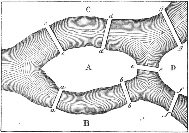
Figure 5-3. The bridges of Königsberg (today, Kaliningrad) in 1759. The illustration is taken from Récréations Mathématiques, vol 1 (Lucas, 1891, p. 22)
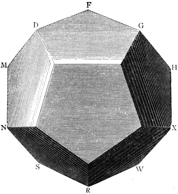
Figure 5-4. A dodecahedron, where the objective is to trace the edges so you visit each vertex exactly once. The illustration is taken from Récréations Mathématiques, vol 2 (Lucas, 1896, p. 205)
ISLAND-HOPPING IN KALININGRAD
Heard of the seven bridges of Königsberg (now known as Kaliningrad)? In 1736, the Swiss mathematician Leonhard Euler came across a puzzle dealing with these, which many of the inhabitants had tried to solve for quite some time. The question was, could you start anywhere in town, cross all seven bridges once, and get back where you started? (You can find the layout of the bridges in Figure 5-3.) To solve the puzzle, Euler decided to abstract away the particulars and . . . invented graph theory. Seems like a good place to start, no?
As you may notice, the structure of the banks and islands in Figure 5-3 is that of a multigraph; for example, there are two edges between A and B and between A and C. That doesn’t really affect the problem. (We could easily invent some imaginary islands in the middle of some of these edges to get an ordinary graph.)
What Euler ended up proving is that it’s possible to visit every edge of a (multi)graph exactly once and end up where you started if and only if the graph is connected and each node has an even degree. The resulting closed walk (roughly, a path where you can visit nodes more than once) is called an Euler tour, or Euler circuit, and such graphs are Eulerian. (You can easily see that the Königsberg isn’t Eulerian; all its vertices are of odd degree.)
It’s not so hard to see that connectedness and even-degree nodes are necessary conditions (disconnectedness is clearly a barrier, and an odd-degree node will necessarily stop your tour at some point). It’s a little less obvious that they are sufficient conditions. We can prove this by induction (big surprise, eh?), but we need to be a bit careful about our induction parameter. If we start removing nodes or edges, the reduced problem may no longer be Eulerian, and our induction hypothesis won’t apply. Let’s not worry about connectivity. If the reduced graph isn’t connected, we can apply the hypothesis to each connected component. But what about the even degrees?
We’re allowed to visit the nodes as often as we want, so what we’ll be removing (or “using up”) is a set of edges. If we remove an even number of edges from each node we visit, out hypothesis will apply. One way of doing this would be to remove the edges of some closed walk (not necessarily visiting all nodes, of course). The question is whether such a closed walk will always exist in an Eulerian graph. If we just start walking from some node, u, every node we enter will go from even degree to odd degree, so we can safely leave it again. As long as we never visit an edge twice, we will eventually get back to u.
Now, let the induction hypothesis be that any connected graph with even-degree nodes and fewer than E edges has a closed walk containing each edge exactly once. We start with E edges and remove the edges of an arbitrary closed walk. We now have one or more Eulerian components, each of which is covered by our hypothesis. The last step is to combine the Euler tours in these components. Our original graph was connected, so the closed walk we removed will necessarily connect the components. The final solution consists of this combined walk, with a “detour” for the Euler tour of each component.
In other words, deciding whether a graph is Eulerian is pretty easy, and finding an Euler tour isn’t that hard either (see Exercise 5-2). The Eulerian tour does, however, have a more problematic relative: the Hamilton cycle.
The Hamilton cycle is named after Sir William Rowan Hamilton, an Irish mathematician (among other things), who proposed it as a game (called The Icosian Game), where the objective is to visit each of the vertices of a dodecahedron (a 12-sided Platonic solid, or d12) exactly once and return to your origin (see Figure 5-4). More generally, a Hamilton cycle is a subgraph containing all the nodes of the full graph (exactly once, as it is a proper cycle). As I’m sure you can see, Königsberg is Hamiltonian (that is, it has a Hamilton cycle). Showing that the dodecahedron is Hamiltonian is a bit harder. In fact, the problem of finding Hamilton paths in general graphs is a hard problem—one for which no efficient algorithm is known (more on this in Chapter 11). Sort of odd, considering how similar the problems are, don’t you think?
A Walk in the Park
It’s late autumn in 1887, and a French telegraphic engineer is wandering through a well-kept garden maze, watching the leaves beginning to turn. As he walks through the passages and intersections of the maze, he recognizes some of the greenery and realizes that he has been moving in a circle. Being an inventive sort, he starts to ponder how he could have avoided this blunder and how he might best find his way out. He remembers being told, as a child, that if he kept turning left at every intersection, he would eventually find his way out, but he can easily see that such a simple strategy won’t work. If his left turns take him back where he started before he gets to the exit, he’s trapped in an infinite cycle. No, he’ll need to find another way. As he finally fumbles his way out of the maze, he has a flash of insight. He rushes home to his notebooks, ready to start sketching out his solution.
OK, this might not be how it actually happened. I admit it, I made it all up, even the year.5 What is true, though, is that a French telegraphic engineer named Trémaux in the late 1880s invented an algorithm for traversing mazes. I’ll get to that in a second, but first let’s explore the “keep turning left” strategy (also known as the left-hand rule) and see how it works—and when it doesn’t.
No Cycles Allowed
Consider the maze in Figure 5-5. As you can see, there are no cycles in it; its underlying structure is that of a tree, as illustrated by the figure on the right. Here the “keep one hand on the wall” strategy will work nicely.6 One way of seeing why it works is to observe that the maze really has only one inner wall (or, to put it another way, if you put wallpaper inside it, you could use one continuous strip). Look at the outer square. As long as you’re not allowed to create cycles, any obstacles you draw have to be connected to it in exactly one place, and this doesn’t create any problems for the left-hand rule. Following this traversal strategy, you’ll discover all nodes and walk every passage twice (once in either direction).
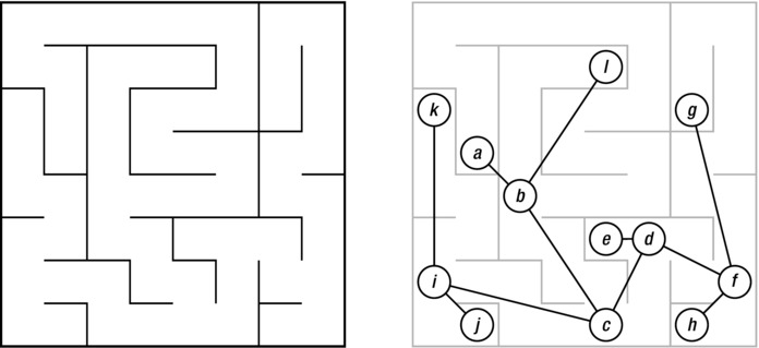
Figure 5-5. A tree, drawn as a maze and as a more conventional graph diagram, superimposed on the maze
The left-hand rule is designed to be executed by an individual actually walking a maze, using only local information. To get a firm grip on what is really going on, we could drop this perspective and formulate the same strategy recursively.7 Once you’re familiar with recursive thinking, such formulations can make it easier to see that an algorithm is correct, and this is one of the easiest recursive algorithms out there. For a basic implementation (which assumes one of our standard graph representations for the tree), see Listing 5-3.
Listing 5-3. Recursive Tree-Traversal
def tree_walk(T, r):                            # Traverse T from root r
    for u in T[r]:                              # For each child. . .
        tree_walk(T, u)                         # ... traverse its subtree
In terms of the maze metaphor, if you’re standing at an intersection and you can go left or right, you first traverse the part of the maze to the left and then the one to the right. And that’s it. It should be obvious (perhaps with the aid of a little induction) that this strategy will traverse the entire maze. Note that only the act of walking forward through each passage is explicitly described here. When you walk the subtree rooted at node u, you walk forward to u and start working on the new passages out from there. Eventually, you will return to the root, r. Going backward like this, over your own tracks, is called backtracking and is implicit in the recursive algorithm. Each time a recursive call returns, you automatically backtrack to the node where the call originated. (Do you see how this backtracking behavior is consistent with the left-hand rule?)
Imagine that someone poked a hole through one of the walls in the maze so that the corresponding graph suddenly had a cycle. Perhaps they busted through the wall just north of the dead end at node e. If you started your walk at e, walking north, you could keep left all you wanted, but you’d never traverse the entire maze—you’d keep walking in circles.8 This is a problem we face when traversing general graphs.9 The general idea in Listing 5-1 gives us a way out of this problem, but before I get into that, let’s see what our French telegraphic engineer came up with.
How to Stop Walking in Circles
Édouard Lucas describes Tremaux’s algorithm for traversing mazes in the first volume of his Récréations Mathématiques in 1891. Lucas writes, in his introduction:10
To completely traverse all the passages of a labyrinth twice, from any initial point, simply follow the rules posed by Trémaux, marking each entry to or exit from an intersection. These rules may be summarized as follows: When possible, avoid passing an intersection you have already visited, and avoid taking passages you have already traversed. Is this not a prudent approach, which also applies in everyday life?
Later in the book, he goes on to describe the method in much more detail, but it is really quite simple, and the previous quote covers the main idea nicely. Instead of marking each entry or exit (say, with a piece of chalk), let’s just say you have muddy boots, so you can see our own tracks (like in Figure 5-2). Trémaux would then tell you to start walking in any direction, backtracking whenever you came to a dead end or an intersection you had already walked through (to avoid cycles). You can’t traverse a passage more than twice (once forward and once backward), so if you’re backtracking into an intersection, you walk forward into one of the unexplored passages, if there are any. If there aren’t any, you keep backtracking (into some other passage with a single set of footprints).11
And that’s the algorithm. One interesting observation to make is that although you can choose several passages for forward traversal, there will always be only one available for backtracking. Do you see why that is? The only way there could be two (or more) would be if you had set off in another direction from an intersection and then come back to it without backtracking. In this case, though, the rules state that you should not enter the intersection but backtrack immediately. (This is also the reason why you’ll never end up traversing a passage twice in the same direction.)
The reason I’ve used the “muddy boots” description here is to make the backtracking really clear; it’s exactly like the one in the recursive tree traversal (which, again, was equivalent to the left-hand rule). In fact, if formulated recursively, Trémaux’s algorithm is just like the tree walk, with the addition of a bit of memory. We know which nodes we have already visited and pretend there’s a wall preventing us from entering them, in effect simulating a tree structure (which becomes our traversal tree).
See Listing 5-4 for a recursive version of Trémaux’s algorithm. In this formulation, it is commonly known as depth-first search, and it is one of the most fundamental (and fundamentally important) traversal algorithms.12
Listing 5-4. Recursive Depth-First Search
def rec_dfs(G, s, S=None):
    if S is None: S = set()                     # Initialize the history
    S.add(s)                                    # We've visited s
    for u in G[s]:                              # Explore neighbors
        if u in S: continue                     # Already visited: Skip
        rec_dfs(G, u, S)                        # New: Explore recursively
Note As opposed to the walk function in Listing 5-1, it would be wrong to use the difference method on G[s] in the loop here because S might change in the recursive call and you could easily end up visiting some nodes multiple times.
Go Deep!
Depth-first search (DFS) gets some of its most important properties from its recursive structure. Once we start working with one node, we make sure we traverse all other nodes we can reach from it before moving on. However, as mentioned in Chapter 4, recursive functions can always be rewritten as iterative ones, possibly simulating the call stack with a stack of our own. Such an iterative formulation of DFS can be useful, both to avoid filling up the call stack and because it might make certain of the algorithm’s properties clearer. Luckily, to simulate recursive traversal, all we need to do is use a stack rather than a set in an algorithm quite like walk in Listing 5-1. Listing 5-5 shows this iterative DFS.
Listing 5-5. Iterative Depth-First Search
def iter_dfs(G, s):
    S, Q = set(), []                            # Visited-set and queue
    Q.append(s)                                 # We plan on visiting s
    while Q:                                    # Planned nodes left?
        u = Q.pop()                             # Get one
        if u in S: continue                     # Already visited? Skip it
        S.add(u)                                # We've visited it now
        Q.extend(G[u])                          # Schedule all neighbors
        yield u                                 # Report u as visited
Beyond the use of a stack (a last-in, first-out, or LIFO, queue, in this case implemented by a list, using append and pop), there are a couple of tweaks here. For example, in my original walk function, the queue was a set, so we’d never risk having the same node scheduled for more than one visit. Once we start using other queue structures, this is no longer the case. I’ve solved this by checking a node for membership in S (that is, whether we’ve already visited the node) before adding its neighbors.
To make the traversal a bit more useful, I’ve also added a yield statement, which will let you iterate over the graph nodes in DFS order. For example, if you had the graph from Figure 2-3 in the variable G, you could try the following:
>>> list(iter_dfs(G, 0))
[0, 5, 7, 6, 2, 3, 4, 1]
One thing worth noting is that I just ran DFS on a directed graph, while I’ve discussed only how it would work on undirected graphs. Actually, both DFS and the other traversal algorithms work just as well for directed graphs. However, if you use DFS on a directed graph, you can’t expect it to explore an entire connected component. For example, for the graph in Figure 2-3, traversing from any other start node than a would mean that a would never be seen because it has no in-edges.
Tip For finding connected components in a directed graph, you can easily construct the underlying undirected graph as a first step. Or you could simply go through the graph and add all the reverse edges. This can be useful for other algorithms as well. Sometimes, you may not even construct the undirected graph; simply considering each edge in both directions when using the directed graph may be sufficient.
You can think of this in terms of Trémaux’s algorithm as well. You’d still be allowed to traverse each (directed) passage both ways, but you’d be allowed to go forward only along the edge direction, and you’d have to backtrack against the edge direction.
In fact, the structure of the iter_dfs function is pretty close to how we might implement the general traversal algorithm hinted at earlier—one where only the queue need be replaced. Let’s beef up walk to the more mature traverse (Listing 5-6).
Listing 5-6. A General Graph Traversal Function
def traverse(G, s, qtype=set):
    S, Q = set(), qtype()
    Q.add(s)
    while Q:
        u = Q.pop()
        if u in S: continue
        S.add(u)
        for v in G[u]:
            Q.add(v)
        yield u
The default queue type here is set, making it similar to the original (arbitrary) walk. You could easily define a stack type (with the proper add and pop methods of our general queue protocol), perhaps like this:
class stack(list):
    add = list.append
The previous depth-first test could then be repeated as follows:
>>> list(traverse(G, 0, stack))
[0, 5, 7, 6, 2, 3, 4, 1]
Of course, it’s also quite OK to implement special-purpose versions of the various traversal algorithms, even though they can be expressed in much the same form.
Depth-First Timestamps and Topological Sorting (Again)
As mentioned earlier, remembering and avoiding previously visited nodes is what keeps us from going in circles (or, rather, cycles), and a traversal without cycles naturally forms a tree. Such traversal trees have different names based on how they were constructed; for DFS, they are aptly named depth-first trees (or DFS trees). As with any traversal tree, the structure of a DFS tree is determined by the order in which the nodes are visited. The thing that is particular to DFS trees is that all descendants of a node u are processed in the time interval from when u is discovered to when we backtrack through it.
To make use of this property, we need to know when the algorithm is backtracking, which can be a bit hard in the iterative version. Although you could extend the iterative DFS from Listing 5-5 to keep track of backtracking (see Exercise 5-7), I’ll be extending the recursive version (Listing 5-4) here. See Listing 5-7 for a version that adds timestamps to each node: one for when it is discovered (discover time, or d) and one for when we backtrack through it (finish time, or f).
Listing 5-7. Depth-First Search with Timestamps
def dfs(G, s, d, f, S=None, t=0):
    if S is None: S = set()                     # Initialize the history
    d[s] = t; t += 1                            # Set discover time
    S.add(s)                                    # We've visited s
    for u in G[s]:                              # Explore neighbors
        if u in S: continue                     # Already visited. Skip
        t = dfs(G, u, d, f, S, t)               # Recurse; update timestamp
    f[s] = t; t += 1                            # Set finish time
    return t                                    # Return timestamp
The parameters d and f should be mappings (dictionaries, for example). The DFS property then states that (1) every node is discovered before its descendants in the DFS tree, and (2) every node is finished after its descendants in the DFS. This follows rather directly from the recursive formulation of the algorithm, but you could easily do an induction proof to convince yourself that it’s true.
One immediate consequence of this property is that we can use DFS for topological sorting, already discussed in Chapter 4. If we perform DFS on a DAG, we could simply sort the nodes based on their descending finish times, and they’d be topologically sorted. Each node u would then precede all its descendants in the DFS tree, which would be any nodes reachable from u, that is, nodes that depend on u. It is in cases like this that it pays to know how an algorithm works. Instead of first calling our timestamping DFS and then sorting afterward, we could simply perform the topological sorting during a custom DFS, by appending nodes when backtracking, as shown in Listing 5-8.13
Listing 5-8. Topological Sorting Based on Depth-First Search
def dfs_topsort(G):
    S, res = set(), []                          # History and result
    def recurse(u):                             # Traversal subroutine
        if u in S: return                       # Ignore visited nodes
        S.add(u)                                # Otherwise: Add to history
        for v in G[u]:
            recurse(v)                          # Recurse through neighbors
        res.append(u)                           # Finished with u: Append it
    for u in G:
        recurse(u)                              # Cover entire graph
    res.reverse()                               # It's all backward so far
    return res
There are a few things that are worth noting in this new topological sorting algorithm. For one thing, I’m explicitly including a for loop over all the nodes to make sure the entire graph is traversed. (Exercise 5-8 asks you to show that this will work.) The check for whether a node is already in the history set (S) is now placed right inside recurse, so we don’t need to put it in both of the for loops. Also, because recurse is an internal function, with access to the surrounding scope (in particular, S and res), the only parameter needed is the node we’re traversing from. Finally, remember that we want the nodes to be sorted in reverse, based on their finish times. That’s why the res list is reversed before it’s returned.
This topsort performs some processing on each node as it backtracks over them (it appends them to the result list). The order in which DFS backtracks over nodes (that is, the order of their finish times) is called postorder, while the order in which it visits them in the first place is called preorder. Processing at these times is called preorder or postorder processing. (Exercise 5-9 asks you to add general hooks for this sort of processing in DFS.)
NODE COLORS AND EDGE TYPES
In describing traversal, I have distinguished between three kinds of nodes: those we don’t know about, those in our queue, and those we’ve visited (and whose neighbors are now in the queue). Some books (such as Introduction to Algorithms, by Cormen et al., mentioned in Chapter 1) introduce a form of node coloring, which is especially important in DFS. Each node is considered white to begin with; they’re gray in the interval between their discover time and their finish time, and they’re black thereafter. You don’t really need this classification in order to implement DFS, but it can be useful in understanding it (or, at least, it might be useful to know about it if you’re going to read a text that uses the coloring).
In terms of Trémaux’s algorithm, gray intersections would be ones we’ve seen but have since avoided; black intersections would be the ones we’ve been forced to enter a second time (while backtracking).
These colors can also be used to classify the edges in the DFS tree. If an edge uv is explored and the node v is white, the edge is a tree edge—that is, it’s part of the traversal tree. If v is gray, it’s a so-called back edge, one that goes back to an ancestor in the DFS tree. Finally, if v is black, the edge is either what is called a forward edge or a cross edge. A forward edge is an edge to a descendant in the traversal tree, while a cross edge is any other edge (that is, not a tree, back or forward edge).
Note that you can classify the edges without actually using any explicit color labeling. Let the time span of a node be the interval from its discover time to its finish time. A descendant will then have a time span contained in its ancestor’s, while nodes unrelated by ancestry will have nonoverlapping intervals. Thus, you can use the timestamps to figure out whether something is, say, a back or forward edge. Even with color labeling, you’d need to consult the timestamps to differentiate between forward and cross edges.
You probably won’t need this classification much, although it does have one important use. If you find a back edge, the graph contains a cycle, but if you don’t, it doesn’t. (Exercise 5-10 asks you to show this.) In other words, you can use DFS to check whether a graph is a DAG (or, for undirected graphs, a tree). Exercise 5-11 asks you to consider how other traversal algorithms would work for this purpose.
Infinite Mazes and Shortest (Unweighted) Paths
Until now, the overeager behavior of DFS hasn’t been a problem. We let it loose in a maze (graph), and it veers off in some direction, as far as it can, before it starts backtracking. This can be problematic, though, if the maze is extremely large. Maybe what we’re looking for, such as an exit, is close to where we started; if DFS sets off in a different direction, it may not return for ages. And if the maze is infinite, it will never get back, even though a different traversal might have found the exit in a matter of minutes. Infinite mazes may sound far-fetched, but they’re actually a close analogy to an important type of traversal problem—that of looking for a solution in a state-space.
But getting lost by being over-eager, like DFS, isn’t only a problem in huge graphs. If we’re looking for the shortest paths (disregarding edge weights, for now) from our start node to all the others, DFS will, most likely, give us the wrong answer. Take a look at the example in Figure 5-6. What happens is that DFS, in its eagerness, keeps going until it reaches c via a detour, as it were. If we want to find the shortest paths to all other nodes (as illustrated in the figure on the right), we need to be more conservative. To avoid taking a detour and reaching a node “from behind,” we need to advance our traversal “fringe” one step at a time. First visit all nodes one step away and then all those two steps away, and so forth.
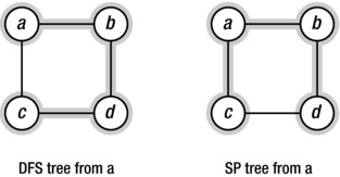
Figure 5-6. Two traversals of a size four cycle. The depth-first tree (highlighted, left) will not necessarily contain minimal paths, as opposed to the shortest path tree (highlighted, right)
In keeping with the maze metaphor, let’s briefly take a look at another maze exploration algorithm, described by Øystein (aka Oystein) Ore in 1959. Just like Trémaux, Ore asks you to make marks at passage entries and exits. Let’s say you start at intersection a. First, you visit all intersections one passage away, each time backtracking to your starting point. If any of the passages you followed were dead ends, you mark them as closed once you return. Any passages leading you to an intersection where you’ve already been are also marked as closed (at both ends).
At this point, you’d like to start exploring all intersections two steps (that is, passages) away. Mark and go through one of the open passages from a; it should now have two marks on it. Let’s say you end up in intersection b. Now, traverse (and mark) all open passages from b, making sure to close them if they lead to dead ends or intersections you’ve already seen. After you’re done, backtrack to a. Once you’ve returned to a, you continue the process with the other open passages, until they’ve all received two marks. (These two marks mean that you’ve traversed intersections two steps away through the passages.)
Let’s jump to step n.14 You’ve visited all intersections n–1 steps away, so all open passages from a now have n–1 marks on them. Open passages at any intersections next to a, such as the b you visited earlier, will have n–2 marks on them, and so forth. To visit all intersections at a distance of n from your starting point, you simply move to all neighbors of a (such as b), adding marks to the passages as you do so, and visit all intersections at a distance n–1 out from them following the same procedure (which will work, by inductive hypothesis).
Once again, using only local information like this might make the bookkeeping a bit tedious (and the explanation a bit confusing). However, just like Trémaux’s algorithm had a very close relative in the recursive DFS, Ore’s method can be formulated in a way that might suit our computer science brains better. The result is something called iterative deepening depth-first search, or IDDFS,15 and it simply consists of running a depth-constrained DFS with an iteratively incremented depth limit.
Listing 5-9 gives a fairly straightforward implementation of IDDFS. It keeps a global set called yielded, consisting of the nodes that have been discovered for the first time and therefore yielded. The inner function, recurse, is basically a recursive DFS with a depth limit, d. If the limit is zero, no further edges are explored recursively. Otherwise, the recursive calls receive a limit of d-1. The main for loop in the iddfs function goes through every depth limit from 0 (just visit, and yield, the start node) to len(G)-1 (the maximum possible depth). If all nodes have been discovered before such a depth is reached, though, the loop is broken.
Listing 5-9. Iterative Deepening Depth-First Search
def iddfs(G, s):
    yielded = set()                             # Visited for the first time
    def recurse(G, s, d, S=None):               # Depth-limited DFS
        if s not in yielded:
            yield s
            yielded.add(s)
        if d == 0: return                       # Max depth zero: Backtrack
        if S is None: S = set()
        S.add(s)
        for u in G[s]:
            if u in S: continue
            for v in recurse(G, u, d-1, S):     # Recurse with depth-1
                yield v
    n = len(G)
    for d in range(n):                          # Try all depths 0..V-1
        if len(yielded) == n: break             # All nodes seen?
        for u in recurse(G, s, d):
            yield u
Note If we were exploring an unbounded graph (such as an infinite state space), looking for a particular node (or a kind of node), we might just keep trying larger depth limits until we found the node we wanted.
It’s not entirely obvious what the running time of IDDFS is. Unlike DFS, it will usually traverse many of the edges and nodes multiple times, so a linear running time is far from guaranteed. For example, if your graph is a path and you start IDDFS from one end, the running time will be quadratic. However, this example is rather pathological; if the traversal tree branches out a bit, most of its nodes will be at the bottom level (as in the knockout tournament in Chapter 3), so for many graphs the running time will be linear or close to linear.
Try running iddfs on a simple graph, and you’ll see that the nodes will be yielded in order from the closest to the furthest from the start node. All with a distance of k are returned, then all with a distance of k + 1, and so forth. If we wanted to find the actual distances, we could easily perform some extra bookkeeping in the iddfs function and yield the distance along with the node. Another way would be to maintain a distance table (similar to the discover and finish times we worked with earlier, for DFS). In fact, we could have one dictionary for distances and one for the parents in the traversal tree. That way, we could retrieve the actual shortest paths, as well as the distances. Let’s focus on the paths for now, and instead of modifying iddfs to include the extra information, we’ll build it into another traversal algorithm: breadth-first search (BFS).
Traversing with BFS is, in fact, quite a bit easier than with IDDFS. You just use the general traversal framework (Listing 5-6) with a first-in first-out queue. This is, in fact, the only salient difference from DFS: we’ve replaced LIFO with FIFO (see Listing 5-10). The consequence is that nodes discovered early will be visited early, and we’ll be exploring the graph level by level, just like in IDDFS. The advantage, though, is that we needn’t visit any nodes or edges multiple times, so we’re back to guaranteed linear performance.16
Listing 5-10. Breadth-First Search
def bfs(G, s):
    P, Q = {s: None}, deque([s])                # Parents and FIFO queue
    while Q:
        u = Q.popleft()                         # Constant-time for deque
        for v in G[u]:
            if v in P: continue                 # Already has parent
            P[v] = u                            # Reached from u: u is parent
            Q.append(v)
    return P
As you can see, the bfs function is similar to iter_dfs, from Listing 5-5. I’ve replaced the list with a deque, and I keep track of which nodes have already received a parent in the traversal tree (that is, they’re in P), rather than remembering which nodes we have visited (S). To extract a path to a node u, you can simply “walk backward” in P:
>>> path = [u]
>>> while P[u] is not None:
...     path.append(P[u])
...     u = P[u]
...
>>> path.reverse()
You are, of course, free to use this kind of parent dictionary in DFS as well, or to use yield to iterate over the nodes in BFS, for that matter. Exercise 5-13 asks you to modify the code to find the distances (rather than the paths).
Tip One way of visualizing BFS and DFS is as browsing the Web. DFS is what you get if you keep following links and then use the Back button once you’re done with a page. The backtracking is a bit like an “undo.” BFS is more like opening every link in a new window (or tab) behind those you already have and then closing the windows as you finish with each page.
There is really only one situation where IDDFS would be preferable over BFS: when searching a huge tree (or some state space “shaped” like a tree). Because there are no cycles, we don’t need to remember which nodes we’ve visited, which means that IDDFS needs only store the path back to the starting node.17 BFS, on the other hand, must keep the entire fringe in memory (as its queue), and as long as there is some branching, this fringe will grow exponentially with the distance to the root. In other words, in these cases IDDFS can save a significant amount of memory, with little or no asymptotic slowdown.
BLACK BOX: DEQUE
As mentioned briefly several times already, Python lists make nice stacks (LIFO queues) but poor (FIFO) queues. Appending to them takes constant time (at least when averaged over many such appends), but popping from (or inserting at) the front takes linear time. What we want for algorithms such as BFS is a double-ended queue, or deque. Such queues are often implemented as linked lists (where appending/prepending and popping at either end are constant-time operations), or so-called circular buffers—arrays where we keep track of the position of both the first element (the head) and the last element (the tail). If either the head or the tail moves beyond its end of the array, we just let it “flow around” to the other side, and we use the mod (%) operator to calculate the actual indices (hence the term circular). If we fill the array completely, we can just reallocate the contents to a bigger one, like with dynamic arrays (see the “Black Box” sidebar on list in Chapter 2).
Luckily, Python has a deque class in the collections module in the standard library. In addition to methods such as append, extend, and pop, which are performed on the right side, it has left equivalents, called appendleft, extendleft, and popleft. Internally, the deque is implemented as a doubly linked list of blocks, each of which is an array of individual elements. Although asymptotically equivalent to using a linked list of individual elements, this reduces overhead and makes it more efficient in practice. For example, the expression d[k] would require traversing the first k elements of the deque d if it were a plain list. If each block contains b elements, you would only have to traverse k//b blocks.
Strongly Connected Components
While traversal algorithms such as DFS, IDDFS, and BFS are useful in their own right, earlier I alluded to the role of traversal as an underlying structure in other algorithms. You’ll see this in many coming chapters, but I’ll end this one with a classical example—a rather knotty problem that can be solved elegantly with some understanding of basic traversal.
The problem is that of finding strongly connected components (SCCs), sometimes known simply as strong components. SCCs are a directed analog for connected components, which I showed you how to find at the beginning of this chapter. A connected component is a maximal subgraph where all nodes can reach each other if you ignore edge directions (or if the graph is undirected). To get strongly connected components, though, you need to follow the edge directions; so, SCCs are the maximal subgraphs where there is a directed path from any node to any other. Finding SCCs and similar structures is an important part of the data flow analysis in modern optimizing compilers, for example.
Consider the graph in Figure 5-7. It is quite similar to the one we started with (Figure 5-1); although there are some additional edges, the SCCs of this new graph consist of the same nodes as the connected components of the undirected original. As you can see, inside the (highlighted) strong components, any node can reach any other, but this property breaks down if you try to add other nodes to any of them.
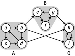
Figure 5-7. A directed graph with three SCCs (highlighted): A, B, and C
Imagine performing a DFS on this graph (possibly traversing from several starting points to ensure you cover the entire graph). Now consider the finish times of the nodes in, say, the strong components A and B. As you can see, there is an edge from A to B, but there is no way to get from B to A. This has consequences for the finish times. You can be certain that A will be finished later than B. That is, the last finish time in A will be later than the last finish time in B. Take a look at Figure 5-7, and it should be obvious why this is so. If you start in B, you can never get into A, so B will finish completely before you even start (let alone finish) your traversal of A. If, however, you start in A, you know that you’ll never get stuck in there (every node can reach every other), so before finishing the traversal, you will eventually migrate to B, and you’ll have to finish that (and, in this case, C) completely before you backtrack to A.
In fact, in general, if there is an edge from any strong component X to another strong component Y, the last finish time in X will be later than the latest in Y. The reasoning is the same as for our example (see Exercise 5-16). I based my conclusion on the fact that you couldn’t get from B to A, though—and this is, in fact, how it works for SCCs in general, because SCCs form a DAG! Therefore, if there’s an edge from X to Y, there will never be any path from Y to X.
Consider the highlighted components in Figure 5-7. If you contract them to single “supernodes” (keeping edges where there were edges originally), you end up with a graph—let’s call it the SCC graph—which looks like this:

This is clearly a DAG, but why will such an SCC graph always be acyclic? Just assume that there is a cycle in the SCC graph. That would mean that you could get from one SCC to another and back again. Do you see a problem with that? Yeah, exactly: every node in the first SCC could reach every node in the second, and vice versa; in fact, all SCCs on such a cycle would combine to form a single SCC, which is a contradiction of our initial assumption that they were separate.
Now, let’s say you flipped all the edges in the graph. This won’t affect which nodes belong together in SCCs (see Exercise 5-15), but it will affect the SCC graph. In our example, you could no longer get out of A. And if you had traversed A and started a new round in B, you couldn’t escape from that, leaving only C. And ... wait a minute ... I just found the strong components there, didn’t I? To apply this idea in general, we always need to start in the SCC without any in-edges in the original graph (that is, with no out-edges after they’re flipped). Basically, we’re looking for the first SCC in a topological sorting of the SCC graph. (And then we’ll move on to the second, and so on.) Looking back at our initial DFS reasoning, that’s where we’d be if we started our traversal with the node that has the latest finish time. In fact, if we choose our starting points for the final traversal by decreasing finish times, we’re guaranteed to fully explore one SCC at the time because we’ll be blocked from moving to the next one by the reverse edges.
This line of reasoning can be a bit tough to follow, but the main idea isn’t all that hard. If there’s an edge from A to B, A will have a later (final) finish time than B. If we choose starting points for our (second) traversal based on decreasing finish times, this means that we’ll visit A before B. Now, if we reverse all the edges, we can still explore all of A, but we can’t move on to B, and this lets us explore a single SCC at a time.
What follows is an outline of the algorithm. Note that instead of “manually” using DFS and sorting the nodes in reverse by finish time, I simply use the dfs_topsort function, which does that job for me.18
- Run dfs_topsort on the graph, resulting in a sequence seq.
- Reverse all edges.
- Run a full traversal, selecting starting points (in order) from seq.
For an implementation of this, see Listing 5-11.
Listing 5-11. Kosaraju’s Algorithm for Finding Strongly Connected Components
def tr(G):                                      # Transpose (rev. edges of) G
    GT = {}
    for u in G: GT[u] = set()                   # Get all the nodes in there
    for u in G:
        for v in G[u]:
            GT[v].add(u)                        # Add all reverse edges
    return GT

def scc(G):
    GT = tr(G)                                  # Get the transposed graph
    sccs, seen = [], set()
    for u in dfs_topsort(G):                    # DFS starting points
        if u in seen: continue                  # Ignore covered nodes
        C = walk(GT, u, seen)                   # Don't go "backward" (seen)
        seen.update(C)                          # We've now seen C
        sccs.append(C)                          # Another SCC found
    return sccs
If you try running scc on the graph in Figure 5-7, you should get the three sets {a, b, c, d}; {e, f, g}; and {i, h}.19 Note that when calling walk, I have now supplied the S parameter to make it avoid the previous SCCs. Because all edges are pointing backward, it would be all too easy to start traversing into these unless that was expressly prohibited.
Note It might seem tempting to drop the call to tr(G), to not reverse all edges and instead reverse the sequence returned by dfs_topsort (that is, to select starting points sorted by ascending rather than descending finish time). That would not work, however (as Exercise 5-17 asks you to show).
The traversal algorithms discussed in this chapter will visit every node they can reach. Sometimes, however, you’re looking for a specific node (or a kind of node), and you’d like to ignore as much of the graph as you can. This kind of search is called goal-directed, and the act of ignoring potential subtrees of the traversal is called pruning. For example, if you knew that the node you were looking for was within k steps of the starting node, running a traversal with a depth limit of k would be a form of pruning. Searching by bisection or in search trees (discussed in Chapter 6) also involves pruning. Rather than traversing the entire search tree, you only visit the subtrees that might contain the value you are looking for. The trees are constructed so that you can usually discard most subtrees at each step, leading to highly efficient algorithms.
Knowledge of where you’re going can also let you choose the most promising direction first (so-called best-first search). An example of this is the A* algorithm, discussed in Chapter 9. If you’re searching a space of possible solutions, you can also evaluate how promising a given direction is (that is, how good is the best solution we could find by following this edge?). By ignoring edges that wouldn’t help you improve on the best you’ve found so far, you can speed things up considerably. This approach is called branch and bound and is discussed in Chapter 11.
Summary
In this chapter, I’ve shown you the basics of moving around in graphs, be they directed or not. This idea of traversal forms the basis—directly or conceptually—for many of the algorithms you’ll learn later in this book and for other algorithms that you’ll probably encounter later. I’ve used examples of maze traversal algorithms (such as Trémaux’s and Ore’s), although they were mainly meant as starting points for more computer-friendly approaches. The general procedure for traversing a graph involves maintaining a conceptual to-do list (a queue) of nodes you’ve discovered, where you check off those that you have actually visited. The list initially contains only the start node, and in each step you visit (and check off) one of the nodes, while adding its neighbors to the list. The ordering (schedule) of items on the list determines, to a large extent, what kind of traversal you are doing: using a LIFO queue (stack) gives depth-first search (DFS), while using a FIFO queue gives breadth-first search (BFS), for example. DFS, which is equivalent to a relatively direct recursive traversal, lets you find discover and finish times for each node, and the interval between these for a descendant will fall inside that of an ancestor. BFS has the useful property that it can be used to find the shortest (unweighted) paths from one node to another. A variation of DFS, called iterative deepening DFS, also has this property, but it is more useful for searching in large trees, such as the state spaces discussed in Chapter 11.
If a graph consists of several connected components, you will need to restart your traversal once for each component. You can do this by iterating over all the nodes, skipping those that have already been visited, and starting a traversal from the others. In a directed graph, this approach may be necessary even if the graph is connected because the edge directions may prevent you from reaching all nodes otherwise. To find the strongly connected components of a directed graph—the parts of the graph where all nodes can reach each other—a slightly more involved procedure is needed. The algorithm discussed here, Kosaraju’s algorithm, involves first finding the finish times for all nodes and then running a traversal in the transposed graph (the graph with all edges reversed), using descending finish times to select starting points.
If You’re Curious ...
If you like traversal, don’t worry. We’ll be doing more of that soon enough. You can also find details on DFS, BFS, and the SCC algorithm discussed in, for example, the book by Cormen et al. (see “References,” Chapter 1). If you’re interested in finding strong components, there are references for Tarjan’s and Gabow’s (or, rather, the Cheriyan-Mehlhorn/Gabow) algorithms in the “References” section of this chapter.
Exercises
5-1. In the components function in Listing 5-2, the set of seen nodes is updated with an entire component at a time. Another option would be to add the nodes one by one inside walk. How would that be different (or, perhaps, not so different)?
5-2. If you’re faced with a graph where each node has an even degree, how would you go about finding an Euler tour?
5-3. If every node in a directed graph has the same in-degree as out-degree, you could find a directed Euler tour. Why is that? How would you go about it, and how is this related to Trémaux’s algorithm?
5-4. One basic operation in image processing is the so-called flood fill, where a region in an image is filled with a single color. In painting applications (such as GIMP or Adobe Photoshop), this is typically done with a paint bucket tool. How would you implement this sort of filling?
5-5. In Greek mythology, when Ariadne helped Theseus overcome the Minotaur and escape the labyrinth, she gave him a ball of fleece thread so he could find his way out again. But what if Theseus forgot to fasten the thread outside on his way in and remembered the ball only once he was thoroughly lost—what could he use it for then?
5-6. In recursive DFS, backtracking occurs when you return from one of the recursive calls. But where has the backtracking gone in the iterative version?
5-7. Write a nonrecursive version of DFS that can deal determine finish times.
5-8. In dfs_topsort (Listing 5-8), a recursive DFS is started from every node (although it terminates immediately if the node has already been visited). How can we be sure that we will get a valid topological sorting, even though the order of the start nodes is completely arbitrary?
5-9. Write a version of DFS where you have hooks (overridable functions) that let the user perform custom processing in pre- and postorder.
5-10. Show that if (and only if) DFS finds no back edges, the graph being traversed is acyclic.
5-11. What challenges would you face if you wanted to use other traversal algorithms than DFS to look for cycles in directed graphs? Why don’t you face these challenges in undirected graphs?
5-12. If you run DFS in an undirected graph, you won’t have any forward or cross edges. Why is that?
5-13. Write a version of BFS that finds the distances from the start node to each of the others, rather than the actual paths.
5-14. As mentioned in Chapter 4, a graph is called bipartite if you can partition the nodes into two sets so that no neighbors are in the same set. Another way of thinking about this is that you’re coloring each node either black or white (for example) so that no neighbors get the same color. Show how you’d find such a bipartition (or two-coloring), if one exists, for any undirected graph.
5-15. If you reverse all the edges of a directed graph, the strongly connected components remain the same. Why is that?
5-16. Let X and Y be two strongly connected components of the same graph, G. Assume that there is at least one edge from X to Y. If you run DFS on G (restarting as needed, until all nodes have been visited), the latest finish time in X will always be later than the latest in Y. Why is that?
5-17. In Kosaraju’s algorithm, we find starting nodes for the final traversal by descending finish times from an initial DFS, and we perform the traversal in the transposed graph (that is, with all edges reversed). Why couldn’t we just use ascending finish times in the original graph?
References
Cheriyan, J. and Mehlhorn, K. (1996). Algorithms for dense graphs and networks on the random access computer. Algorithmica, 15(6):521-549.
Littlewood, D. E. (1949). The Skeleton Key of Mathematics: A Simple Account of Complex Algebraic Theories. Hutchinson & Company, Limited.
Lucas, É. (1891). Récréations Mathématiques, volume 1, second edition. Gauthier-Villars et fils, Imprimeurs-Libraires. Available online at http://archive.org.
Lucas, É. (1896). Récréations Mathématiques, volume 2, second edition. Gauthier-Villars et fils, Imprimeurs-Libraires. Available online at http://archive.org.
Ore, O. (1959). An excursion into labyrinths. Mathematics Teacher, 52:367-370.
Tarjan, R. (1972). Depth-first search and linear graph algorithms. SIAM Journal on Computing, 1(2): 146-160.
__________________
1I’ve “stolen” the subtitle for this chapter from Dudley Ernest Littlewood’s The Skeleton Key of Mathematics.
2If you’re not a gamer, feel free to imagine this as your office building, dream home, or whatever strikes your fancy.
3I’ll be using dicts with adjacency sets as the default representation in the following, although many of the algorithms will work nicely with other representations from Chapter 2 as well. Usually, rewriting an algorithm to use a different representation isn’t too hard either.
4This is the running time of all the traversal algorithms in this chapter, except (sometimes) IDDFS.
5Hey, even the story of Newton and the apple is apocryphal.
6Tracing your tour from a, you should end up with the node sequence a, b, c, d, e, f, g, h, d, c, i, j, i, k, i, c, b, l, b, a.
7This recursive version would be harder to use if you were actually faced with a real-life maze, of course.
8And just like that, a spelunker can turn troglodyte.
9People seem to end up walking in circles when wandering in the wild as well. And research by the U.S. Army suggests that people prefer going south, for some reason (as long as they have their bearings). Neither strategy is particularly helpful if you’re aiming for a complete traversal, of course.
10My translation.
11You can perform the same procedure even if your boots aren’t muddy. Just make sure to clearly mark entries and exits (say, with a piece of chalk). In this case, it’s important to make two marks when you come to an old intersection and immediately start backtracking.
12In fact, in some contexts, the term backtracking is used as a synonym for recursive traversal, or depth-first search.
13The dfs_topsort function can also be used to sort the nodes of a general graph by decreasing finish times, as needed when looking for strongly connected components, discussed later in this chapter.
14In other words, let’s think inductively.
15IDDFS isn’t completely equivalent to Ore’s method because it doesn’t mark edges as closed in the same way. Adding that kind of marking is certainly possible and would be a form of pruning, discussed later in this chapter.
16On the other hand, we’ll be jumping from node to node in a manner that could not possibly be implemented in a real-life maze.
17To have any memory savings, you’d have to remove the S set. Because you’d be traversing a tree, that wouldn’t cause any trouble (that is, traversal cycles).
18This might seem like cheating because I’m using topological sorting on a non-DAG. The idea is just to get the nodes sorted by decreasing finish time, though, and that’s exactly what dfs_topsort does—in linear time.
19Actually, walk will return a traversal tree for each strong component.