Table of Contents for
Python Algorithms: Mastering Basic Algorithms in the Python Language, Second Edition
 Python Algorithms: Mastering Basic Algorithms in the Python Language, Second Edition
Published by
Apress, 2015
Python Algorithms: Mastering Basic Algorithms in the Python Language, Second Edition
Published by
Apress, 2015
- Cover
- Title
- Copyright
- Dedication
- Contents at a Glance
- Contents
- About the Author
- About the Technical Reviewer
- Acknowledgments
- Preface
- Chapter 1: Introduction
- Chapter 2: The Basics
- Chapter 3: Counting 101
- Chapter 4: Induction and Recursion … and Reduction
- Chapter 5: Traversal: The Skeleton Key of Algorithmics
- Chapter 6: Divide, Combine, and Conquer
- Chapter 7: Greed Is Good? Prove It!
- Chapter 8: Tangled Dependencies and Memoization
- Chapter 9: From A to B with Edsger and Friends
- Chapter 10: Matchings, Cuts, and Flows
- Chapter 11: Hard Problems and (Limited) Sloppiness
- Appendix A: Pedal to the Metal: Accelerating Python
- Appendix B: List of Problems and Algorithms
- Appendix C: Graph Terminology
- Appendix D: Hints for Exercises
- Index

Divide, Combine, and Conquer
Divide and rule, a sound motto;
Unite and lead, a better one.
— Johann Wolfgang von Goethe, Gedichte
This chapter is the first of three dealing with well-known design strategies. The strategy dealt with in this chapter, divide and conquer (or simply D&C), is based on decomposing your problem in a way that improves performance. You divide the problem instance, solve subproblems recursively, combine the results, and thereby conquer the problem—a pattern that is reflected in the chapter title.1
Tree-Shaped Problems: All About the Balance
I have mentioned the idea of a subproblem graph before: We view subproblems as nodes and dependencies (or reductions) as edges. The simplest structure such a subproblem graph can have is a tree. Each subproblem may depend on one or more others, but we’re free to solve these other subproblems independently of each other. (When we remove this independence, we end up with the kind of overlap and entanglements dealt with in Chapter 8.) This straightforward structure means that as long as we can find the proper reduction, we can implement the recursive formulation of our algorithm directly.
You already have all the puzzle pieces needed to understand the idea of divide-and-conquer algorithms. Three ideas that I’ve already discussed cover the essentials:
- Divide-and-conquer recurrences, in Chapter 3
- Strong induction, in Chapter 4
- Recursive traversal, in Chapter 5
The recurrences tell you something about the performance involved, the induction gives you a tool for understanding how the algorithms work, and the recursive traversal (DFS in trees) is a raw skeleton for the algorithms.
Implementing the recursive formulation of our induction step directly is nothing new. I showed you how some simple sorting algorithms could be implemented that way in Chapter 4, for example. The one crucial addition in the design method of divide and conquer is balance. This is where strong induction comes in: Instead of recursively implementing the step from n-1 to n, we want to go from n/2 to n. That is, we take solutions of size n/2 and build a solution of size n. Instead of (inductively) assuming that we can solve subproblems of size n-1, we assume that we can deal with all subproblems of sizes smaller than n.
What does this have to do with balance, you ask? Think of the weak induction case. We’re basically dividing our problem in two parts: one of size n-1 and one of size 1. Let’s say the cost of the inductive step is linear (a quite common case). Then this gives us the recurrence T(n) = T(n-1) + T(1) + n. The two recursive calls are wildly unbalanced, and we end up, basically, with our handshake recurrence, with a resulting quadratic running time. What if we managed to distribute the work more evenly among our two recursive calls? That is, could we reduce the problem to two subproblems of similar size? In that case, the recurrence turns into T(n) = 2T(n/2) + n. This should also be quite familiar: It’s the canonical divide-and-conquer recurrence, and it yields a loglinear (Θ(n lg n)) running time—a huge improvement.
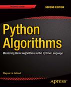
Figures 6-1 and 6-2 illustrate the difference between the two approaches, in the form of recursion trees. Note that the number of nodes is identical—the main effect comes from the distribution of work over those nodes. This may seem like a conjuror’s trick; where does the work go? The important realization is that for the simple, unbalanced stepwise approach (Figure 6-1), many of the nodes are assigned a high workload, while for the balanced divide-and-conquer approach (Figure 6-2), most nodes have very little work to do. For example, in the unbalanced recursion, there will always be roughly a quarter of the calls that each has a cost of at least n/2, while in the balanced recursion, there will be only three, no matter the value of n. That’s a pretty significant difference.
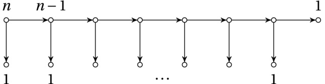
Figure 6-1. An unbalanced decomposition, with linear division/combination cost and quadratic running time in total
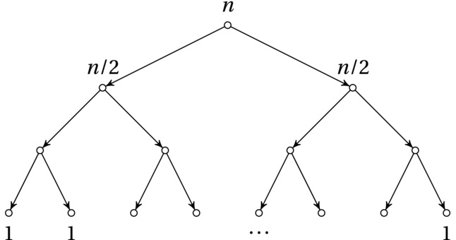
Figure 6-2. Divide and conquer: a balanced decomposition, with linear division/combination cost and loglinear running time in total
Let’s try to recognize this pattern in an actual problem. The skyline problem2 is a rather simple example. You are given a sorted sequence of triples (L,H,R), where L is the left x-coordinate of a building, H is its height, and R is its right x-coordinate. In other words, each triple represents the (rectangular) silhouette of a building, from a given vantage point. Your task is to construct a skyline from these individual building silhouettes.
Figures 6-3 and 6-4 illustrate the problem. In Figure 6-4, a building is being added to an existing skyline. If the skyline is stored as a list of triples indicating the horizontal line segments, adding a new building can be done in linear time by (1) looking for the left coordinate of the building in the skyline sequence and (2) elevating all that are lower than this building, until (3) you find the right coordinate of the building. If the left and right coordinates of the new building are in the middle of some horizontal segments, they’ll need to be split in two. For simplicity, we can assume that we start with a zero-height segment covering the entire skyline.
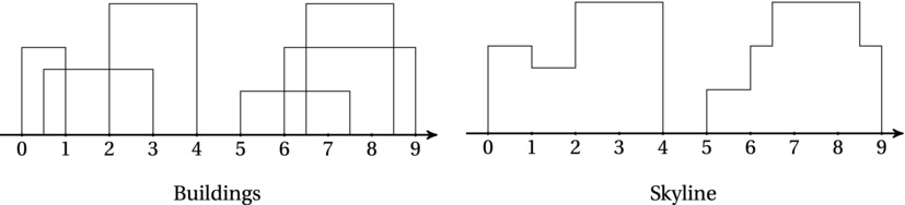
Figure 6-3. A set of building silhouettes and the resulting skyline
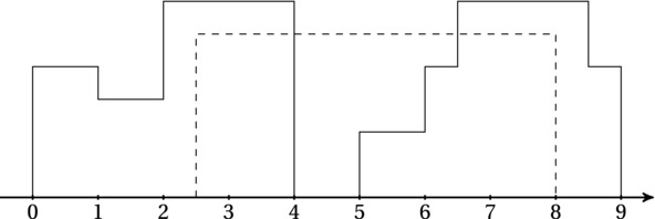
Figure 6-4. Adding a building (dashed) to a skyline (solid)
The details of this merging aren’t all that important here. The point is that we can add a building to the skyline in linear time. Using simple (weak) induction, we now have our algorithm: We start with a single building and keep adding new ones until we’re done. And, of course, this algorithm has a quadratic running time. To improve this, we want to switch to strong induction—divide and conquer. We can do this by noting that merging two skylines is no harder than merging one building with a skyline: We just traverse the two in “lockstep,” and wherever one has a higher value than the other, we use the maximum, splitting horizontal line segments where needed. Using this insight, we have our second, improved algorithm: To create a skyline for all the buildings, first (recursively) create two skylines, based on half the buildings each, and then merge them. This algorithm, as I’m sure you can see, has a loglinear running time. Exercise 6-1 asks you to actually implement this algorithm.
The Canonical D&C Algorithm
The recursive skyline algorithm hinted at in the previous section exemplifies the prototypical way a divide-and-conquer algorithm works. The input is a set (perhaps a sequence) of elements; the elements are partitioned, in at most linear time, into two sets of roughly equal size, the algorithm is run recursively on each half, and the results are combined, also in at most linear time. It’s certainly possible to modify this standard form (you’ll see an important variation in the next section), but this schema encapsulates the core idea.
Listing 6-1 sketches out a general divide-and-conquer function. Chances are you’ll be implementing a custom version for each algorithm, rather than using a general function such as this, but it does illustrate how these algorithms work. I’m assuming here that it’s OK to simply return S in the base case; that depends on how the combine function works, of course.3
Listing 6-1. A General Implementation of the Divide-and-Conquer Scheme
def divide_and_conquer(S, divide, combine):
    if len(S) == 1: return S
    L, R = divide(S)
    A = divide_and_conquer(L, divide, combine)
    B = divide_and_conquer(R, divide, combine)
    return combine(A, B)
Figure 6-5 is another illustration of the same pattern. The upper half of the figure represents the recursive calls, while the lower half represents the way return values are combined. Some algorithms (such as quicksort, described later in this chapter) do most of their work in the upper half (division), while some are more active in the lower (combination). The perhaps most well-known example of an algorithm with a focus on combination is merge sort (described a bit later in this chapter), which is also a prototypical example of a divide-and-conquer algorithm.
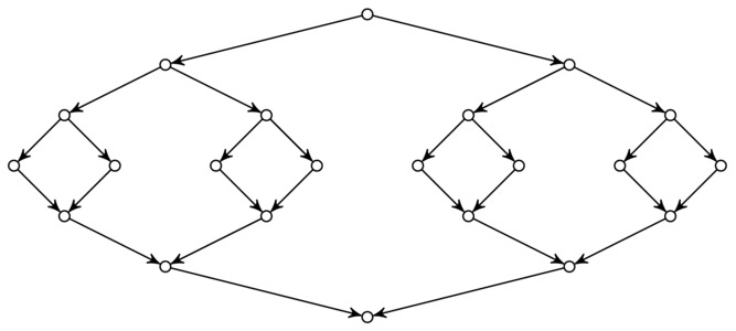
Figure 6-5. Dividing, recursing, and combining in a divide-and-conquer algorithm
Searching by Halves
Before working through some more examples that fit the general pattern, let’s look at a related pattern, which discards one of the recursive calls. You’ve already seen this in my earlier mentions of binary search (bisection): It divides the problem into two equal halves and then recurses on only one of those halves. The core principle here is still balance. Consider what would happen in a totally unbalanced search. If you recall the “think of a particle” game from Chapter 3, the unbalanced solution would be equivalent to asking “Is this your particle?” for each particle in the universe. The difference is still encapsulated by Figures 6-1 and 6-2, except the work in each node (for this problem) is constant, and we only actually perform the work along a path from the root to a leaf.
Binary search may not seem all that interesting. It’s efficient, sure, but searching through a sorted sequence ... isn’t that sort of a limited area of application? Well, no, not really. First, that operation in itself can be important as a component in other algorithms. Second, and perhaps as importantly, binary search can be a more general approach to looking for things. For example, the idea can be used for numerical optimization, such as with Newton’s method, or in debugging your code. Although “debugging by bisection” can be efficient enough when done manually (“Does the code crash before it reaches this print statement?”), it is also used in some revision control systems (RCSs), such as Mercurial and Git.
It works like this: You use an RCS to keep track of changes in your code. It stores many different versions, and you can “travel back in time,” as it were, and examine old code at any time. Now, say you encounter a new bug, and you understandably enough want to find it. How can your RCS help? First, you write a test for your test suite—one that will detect the bug if it’s there. (That’s always a good first step when debugging.) You make sure to set up the test so that the RCS can access it. Then you ask the RCS to look for the place in your history where the bug appeared. How does it do that? Big surprise: by binary search. Let’s say you know the bug appeared between revisions 349 and 574. The RCS will first revert your code to revision 461 (in the middle between the two) and run your test. Is the bug there? If so, you know it appeared between 349 and 461. If not, it appeared between 462 and 574. Lather, rinse, repeat.
This isn’t just a neat example of what bisection can be used for; it also illustrates a couple of other points nicely. First, it shows that you can’t always use stock implementations of known algorithms, even if you’re not really modifying them. In a case such as this, chances are that the implementors behind your RCS had to implement the binary search themselves. Second, it’s a good example of a case where reducing the number of basic operations can be crucial—more so than just implementing things efficiently. Compiling your code and running the test suite is likely to be slow anyway, so you’d like to do this as few times as possible.
BLACK BOX: BISECT
Binary search can be applied in many settings, but the straight “search for a value on a sorted sequence” version is available in the standard library, in the bisect module. It contains the bisect function, which works as expected:
>>> from bisect import bisect
>>> a = [0, 2, 3, 5, 6, 8, 8, 9]
>>> bisect(a, 5)
4
Well, it’s sort of what you’d expect ... it doesn’t return the position of the 5 that’s already there. Rather, it reports the position to insert the new 5, making sure it’s placed after all existing items with the same value. In fact, bisect is another name for bisect_right, and there’s also a bisect_left:
>>> from bisect import bisect_left
>>> bisect_left(a, 5)
3
The bisect module is implemented in C, for speed, but in earlier versions (prior to Python 2.4) it was actually a plain Python module, and the code for bisect_right was as follows (with my comments):
def bisect_right(a, x, lo=0, hi=None):
if hi is None: # Searching to the end
hi = len(a)
while lo < hi: # More than one possibility
mid = (lo+hi)//2 # Bisect (find midpoint)
if x < a[mid]: hi = mid # Value < middle? Go left
else: lo = mid+1 # Otherwise: go right
return lo
As you can see, the implementation is iterative, but it’s entirely equivalent to the recursive version.
There is also another pair of useful functions in this module: insort (alias for insort_right) and insort_left. These functions find the right position, like their bisect counterparts, and then actually insert the element. While the insertion is still a linear operation, at least the search is logarithmic (and the actual insertion code is pretty efficiently implemented).
Sadly, the various functions of the bisect library don’t support the key argument, used in list.sort, for example. You can achieve similar functionality with the so-called decorate, sort, undecorate (or, in this case, decorate, search, undecorate) pattern, or DSU for short:
>>> seq = "I aim to misbehave".split()
>>> dec = sorted((len(x), x) for x in seq)
>>> keys = [k for (k, v) in dec]
>>> vals = [v for (k, v) in dec]
>>> vals[bisect_left(keys, 3)]
'aim'
Or, you could do it more compactly:
>>> seq = "I aim to misbehave".split()
>>> dec = sorted((len(x), x) for x in seq)
>>> dec[bisect_left(dec, (3, ""))][1]
'aim'
As you can see, this involves creating a new, decorated list, which is a linear operation. Clearly, if we do this before every search, there’d be no point in using bisect. If, however, we can keep the decorated list between searches, the pattern can be useful. If the sequence isn’t sorted to begin with, we can perform the DSU as part of the sorting, as in the previous example.
Traversing Search Trees ... with Pruning
Binary search is the bee’s knees. It’s one of the simplest algorithms out there, but it really packs a punch. There is one catch, though: To use it, your values must be sorted. Now, if we could keep them in a linked list, that wouldn’t be a problem. For any object we wanted to insert, we’d just find the position with bisection (logarithmic) and then insert it (constant). The problem is—that won’t work. Binary search needs to be able to check the middle value in constant time, which we can’t do with a linked list. And, of course, using an array (such as Python’s lists) won’t help. It’ll help with the bisection, but it ruins the insertion.
If we want a modifiable structure that’s efficient for search, we need some kind of middle ground. We need a structure that is similar to a linked list (so we can insert elements in constant time) but that still lets us perform a binary search. You may already have figured the whole thing out, based on the section title, but bear with me. The first thing we need when searching is to access the middle item in constant time. So, let’s say we keep a direct link to that. From there, we can go left or right, and we’ll need to access the middle element of either the left half or the right half. So ... we can just keep direct links from the first item to these two, one “left” reference and one “right” reference.
In other words, we can just represent the structure of the binary search as an explicit tree structure! Such a tree would be easily modifiable, and we could traverse it from root to leaf in logarithmic time. So, searching is really our old friend traversal—but with pruning. We wouldn’t want to traverse the entire tree (resulting in a so-called linear scan). Unless we’re building the tree from a sorted sequence of values, the “middle element of the left half” terminology may not be all that helpful. Instead, we can think of what we need to implement our pruning. When we look at the root, we need to be able to prune one of the subtrees. (If we found the value we wanted in an internal node and the tree didn’t contain duplicates, we wouldn’t continue in either subtree, of course.)
The one thing we need is the so-called search tree property: For a subtree rooted at r, all the values in the left subtree are smaller than (or equal to) the value of r, while those in the right subtree are greater. In other words, the value at a subtree root bisects the subtree. An example tree with this property is shown in Figure 6-6, where the node labels indicate the values we’re searching. A tree structure like this could be useful in implementing a set; that is, we could check whether a given value was present. To implement a mapping, however, each node would contain both a key, which we searched for, and a value, which was what we wanted.

Figure 6-6. A (perfectly balanced) binary search tree, with the search path for 11 highlighted
Usually, you don’t build a tree in bulk (although that can be useful at times); the main motivation for using trees is that they’re dynamic, and you can add nodes one by one. To add a node, you search for where it should have been and then add it as a new leaf there. For example, the tree in Figure 6-6 might have been built by initially adding 8 and then 12, 14, 4, and 6, for example. A different ordering might have given a different tree.
Listing 6-2 gives you a simple implementation of a binary search tree, along with a wrapper that makes it look a bit like a dict. You could use it like this, for example:
>>> tree = Tree()
>>> tree["a"] = 42
>>> tree["a"]
42
>>>  "b" in tree
False
As you can see, I’ve implemented insertion and search as free-standing functions, rather than methods. That’s so that they’ll work also on None nodes. (You don’t have to do it like that, of course.)
Listing 6-2. Insertion into and Search in a Binary Search Tree
class Node:
    lft = None
    rgt = None
    def __init__(self, key, val):
        self.key = key
        self.val = val

def insert(node, key, val):
    if node is None: return Node(key, val)      # Empty leaf: add node here
    if node.key == key: node.val = val          # Found key: replace val
    elif key < node.key:                        # Less than the key?
        node.lft = insert(node.lft, key, val)   # Go left
    else:                                       # Otherwise...
        node.rgt = insert(node.rgt, key, val)   # Go right
    return node

def search(node, key):
    if node is None: raise KeyError             # Empty leaf: it's not here
    if node.key == key: return node.val         # Found key: return val
    elif key < node.key:                        # Less than the key?
        return search(node.lft, key)            # Go left
    else:                                       # Otherwise...
        return search(node.rgt, key)            # Go right

class Tree:                                     # Simple wrapper
    root = None
    def __setitem__(self, key, val):
        self.root = insert(self.root, key, val)
    def __getitem__(self, key):
        return search(self.root, key)
    def __contains__(self, key):
        try: search(self.root, key)
        except KeyError: return False
        return True
 Note The implementation in Listing 6-2 does not permit the tree to contain duplicate keys. If you insert a new value with an existing key, the old value is simply overwritten. This could easily be changed because the tree structure itself does not preclude duplicates.
SORTED ARRAYS, TREES, AND DICTS: CHOICES, CHOICES
Bisection (on sorted arrays), binary search trees, and dicts (that is, hash tables) all implement the same basic functionality: They let you search efficiently. There are some important differences, though. Bisection is fast, with little overhead, but works only on sorted arrays (such as Python lists). And sorted arrays are hard to maintain; adding elements takes linear time. Search trees have more overhead but are dynamic and let you insert and remove elements. In many cases, though, the clear winner will be the hash table, in the form of dict. Its average asymptotic running time is constant (as opposed to the logarithmic running time of bisection and search trees), and it is close to that in practice, with little overhead.
Hashing requires you to be able to compute a hash value for your objects. In practice, you can almost always do this, but in theory, bisection and search trees are a bit more flexible here—they need only to compare objects and figure out which one is smaller.4 This focus on ordering also means that search trees will let you access your values in sorted order—either all of them or just a portion. Trees can also be extended to work in multiple dimensions (to search for points inside a hyperrectangular region) or to even stranger forms of search criteria, where hashing may be hard to achieve. There are more common cases, too, when hashing isn’t immediately applicable. For example, if you want the entry that is closest to your lookup key, a search tree would be the way to go.
Selection
I’ll round off this section on “searching by half” with an algorithm you may not end up using a lot in practice but that takes the idea of bisection in an interesting direction. Besides, it sets the stages for quicksort (next section), which is one of the classics.
The problem is to find the kth largest number in an unsorted sequence, in linear time. The most important case is, perhaps, to find the median—the element that would have been in the middle position (that is, (n+1)//2), had the sequence been sorted.5 Interestingly, as a side effect of how the algorithm works, it will also allow us to identify which objects are smaller than the object we seek. That means we’ll be able to find the k smallest (and, simultaneously, the n-k largest) elements with a running time of Θ(n), meaning that the value of k doesn’t matter!
This may be stranger than it seems at first glance. The running time constraint rules out sorting (unless we can count occurrences and use counting sort, as discussed in Chapter 4). Any other obvious algorithm for finding the k smallest objects would use some data structure to keep track of them. For example, you could use an approach similar to insertion sort: Keep the k smallest objects found so far either at the beginning of the sequence or in a separate sequence.
If you kept track of which one of them was largest, checking each large object in the main sequence would be fast (just a constant-time check). If you needed to add an object, though, and you already had k, you’d have to remove one. You’d remove the largest, of course, but then you’d have to find out which one was now largest. You could keep them sorted (that is, stay close to insertion sort), but the running time would be Θ(nk) anyway.
One step up from this (asymptotically) would be to use a heap, essentially transforming our “partial insertion sort” into a “partial heap sort,” making sure that there are never more than k elements in the heap. (See the “Black Box” sidebar about binary heaps, heapq, and heapsort for more information.) This would give you a running time of Θ(n lg k), and for a reasonably small k, this is almost identical to Θ(n), and it lets you iterate over the main sequence without jumping around in memory, so in practice it might be the solution of choice.
Tip If you’re looking for the k smallest (or largest) objects in an iterable in Python, you would probably use the nsmallest (or nlargest) function from the heapq module if your k is small, relative to the total number of objects. If the k is large, you should probably sort the sequence (either using the sort method or using the sorted function) and pick out the k first objects. Time your results to see what works best—or just choose the version that makes your code as clear as possible.
So, how can we take the next step, asymptotically, and remove dependence on k altogether? It turns out that guaranteeing a linear worst case is a bit knotty, so let’s focus on the average case. Now, if I tell you to try applying the idea of divide and conquer, what would you do? A first clue might be that we’re aiming for a linear running time; what “divide by half” recurrence does that? It’s the one with a single recursive call (which is equivalent to the knockout tournament sum): T(n) = T(n/2) + n. In other words, we divide the problem in half (or, for now, in half on average) by performing linear work, just like the more canonical divide-and-conquer approach, but we manage to eliminate one half, taking us closer to binary search. What we need to figure out, in order to design this algorithm, is how to partition the data in linear time so that we end up with all our objects in one half.
As always, systematically going through the tools at our disposal, and framing the problem as clearly as we can, makes it much easier to figure out a solution. We’ve arrived at a point where what we need is to partition a sequence into two halves, one consisting of small values and one of large values. And we don’t have to guarantee that the halves are equal—only that they’ll be equal on average. A simple way of doing this is to choose one of the values as a so-called pivot and use it to divide the others: All those smaller than (or equal to) the pivot end up in the left half, while those larger end up on the right. Listing 6-3 gives you a possible implementation of partition and select. Note that this version of partition is primarily meant to be readable; Exercise 6-11 asks you to see whether you can remove some overhead. The way select is written here, it returns the kth smallest element; if you’d rather have all the k smallest elements, you can simply rewrite it to return lo instead of pi.
Listing 6-3. A Straightforward Implementation of Partition and Select
def partition(seq):
    pi, seq = seq[0], seq[1:]                   # Pick and remove the pivot
    lo = [x for x in seq if x <= pi]            # All the small elements
    hi = [x for x in seq if x > pi]             # All the large ones
    return lo, pi, hi                           # pi is "in the right place"

def select(seq, k):
    lo, pi, hi = partition(seq)                 # [<= pi], pi, [>pi]
    m = len(lo)
    if m == k: return pi                        # We found the kth smallest
    elif m < k:                                 # Too far to the left
        return select(hi, k-m-1)                # Remember to adjust k
    else:                                       # Too far to the right
        return select(lo, k)                    # Just use original k here
SELECTING IN LINEAR TIME, GUARANTEED!
The selection algorithm implemented in this section is known as randomized select (although the randomized version usually chooses the pivot more randomly than here; see Exercise 6-13). It lets you do selection (for example, find the median) in linear expected time, but if the pivot choices are poor at each step, you end up with the handshake recurrence (linear work, but reducing size by only 1) and thereby quadratic running time. While such an extreme result is unlikely in practice (though, again, see Exercise 6-13), you can in fact avoid it also in the worst case.
It turns out guaranteeing that the pivot is even a small percentage into the sequence (that is, not at either end, or a constant number of steps from it) is enough for the running time to be linear. In 1973, a group of algorists (Blum, Floyd, Pratt, Rivest, and Tarjan) came up with a version of the algorithm that gives exactly this kind of guarantee.
The algorithm is a bit involved, but the core idea is simple enough: First divide the sequence into groups of five, or some other small constant. Find the median in each, using, for example, a simple sorting algorithm. So far, we’ve used only linear time. Now, find the median among these medians, using the linear selection algorithm recursively. This will work, because the number of medians is smaller than the size of the original sequence—still a bit mind-bending. The resulting value is a pivot that is guaranteed to be good enough to avoid the degenerate recursion—use it as a pivot in your selection.
In other words, the algorithm is used recursively in two ways: first, on the sequence of medians, to find a good pivot, and second, on the original sequence, using this pivot.
While the algorithm is important to know about for theoretical reasons because it means selection can be done in guaranteed linear time, you’ll probably never actually use it in practice.
Sorting by Halves
Finally, we’ve arrived at the topic most commonly associated with the divide-and-conquer strategy: sorting. I’m not going to delve into this too deeply, because Python already has one of the best sorting algorithms ever devised (see the “Black Box” sidebar about timsort, later in this section), and its implementation is highly efficient. In fact, list.sort is so efficient, you’d probably consider it as a first choice in place of other, asymptotically slightly better algorithms (for example, for selection). Still, the sorting algorithms in this section are among the most well-known algorithms, so you should understand how they work. Also, they are a great example of the way divide and conquer is used to design algorithms.
Let’s first consider one of the celebrities of algorithm design: C. A. R. Hoare’s quicksort. It’s closely related to the selection algorithm from the previous section, which is also due to Hoare (and sometimes called quickselect). The extension is simple: If quickselect represents traversal with pruning—finding a path in the recursion tree down to the kth smallest element—then quicksort represents a full traversal, which means finding a solution for every k. Which is the smallest element? The second smallest? And so forth. By putting them all in their place, the sequence is sorted. Listing 6-4 shows a version of quicksort.
Listing 6-4. Quicksort
def quicksort(seq):
    if len(seq) <= 1: return seq                # Base case
    lo, pi, hi = partition(seq)                 # pi is in its place
    return quicksort(lo) + [pi] + quicksort(hi) # Sort lo and hi separately
As you can see, the algorithm is simple, as long as you have partition in place. (Exercises 6-11 and 6-12 ask you to rewrite quicksort and partition to yield an in-place sorting algorithm.) First, it splits the sequence into those we know must be to the left of pi and those that must be to the right. These two halves are then sorted recursively (correct by inductive assumption). Concatenating the halves, with the pivot in the middle, is guaranteed to result in a sorted sequence. Because we’re not guaranteed that partition will balance the recursion properly, we know only that quicksort is loglinear in the average case—in the worst case it’s quadratic.6
Quicksort is an example of a divide-and-conquer algorithm that does its main work before the recursive calls, in dividing its data (using partition). The combination part is trivial. We can do it the other way around, though: trivially split our data down the middle, guaranteeing a balanced recursion (and a nice worst-case running time), and then make an effort at combining, or merging the results. This is exactly what merge sort does. Just like our skyline algorithm from the beginning of this chapter goes from inserting a single building to merging two skylines, merge sort goes from inserting a single element in a sorted sequence (insertion sort) to merging two sorted sequences.
You’ve already seen the code for merge sort in Chapter 3 (Listing 3-2), but I’ll repeat it here, with some comments (Listing 6-5).
Listing 6-5. Merge Sort
def mergesort(seq):
    mid = len(seq)//2                           # Midpoint for division
    lft, rgt = seq[:mid], seq[mid:]
    if len(lft) > 1: lft = mergesort(lft)       # Sort by halves
    if len(rgt) > 1: rgt = mergesort(rgt)
    res = []
    while lft and rgt:                          # Neither half is empty
        if lft[-1] >=rgt[-1]:                   # lft has greatest last value
            res.append(lft.pop())               # Append it
        else:                                   # rgt has greatest last value
            res.append(rgt.pop())               # Append it
    res.reverse()                               # Result is backward
    return (lft or rgt) + res                   # Also add the remainder
Understanding how this works should be a bit easier now than it was in Chapter 3. Note the merging part has been written to show what’s going on here. If you were to actually use merge sort (or a similar algorithm) in Python, you would probably use heapq.merge to do the merging.
BLACK BOX: TIMSORT
The algorithm hiding in list.sort is one invented (and implemented) by Tim Peters, one of the big names in the Python community.7 The algorithm, aptly named timsort, replaces an earlier algorithm that had lots of tweaks to handle special cases such as segments of ascending and descending values, and the like. In timsort, these cases are handled by the general mechanism, so the performance is still there (and in some cases, it’s much improved), but the algorithm is cleaner and simpler. The algorithm is still a bit too involved to explain in detail here; I’ll try to give you a quick overview. For more details, take a look at the source.8
Timsort is a close relative to merge sort. It’s an in-place algorithm, in that it merges segments and leaves the result in the original array (although it uses some auxiliary memory during the merging). Instead of simply sorting the array half-and-half and then merging those, though, it starts at the beginning, looking for segments that are already sorted (possibly in reverse), called runs. In random arrays, there won’t be many, but in many kinds of real data, there may be a lot—giving the algorithm a clear edge over a plain merge sort and a linear running time in the best case (and that covers a lot of cases beyond simply getting a sequence that’s already sorted).
As timsort iterates over the sequence, identifying runs and pushing their bounds onto a stack, it uses some heuristics to decide which runs are to be merged when. The idea is to avoid the kind of merge imbalance that would give you a quadratic running time while still exploiting the structure in the data (that is, the runs). First, any really short runs are artificially extended and sorted (using a stable insertion sort). Second, the following invariants are maintained for the three topmost runs on the stack, A, B, and C (with A on top): len(A) > len(B) + len(C) and len(B) > len(C). If the first invariant is violated, the smaller of A and C is merged with B, and the result replaces the merged runs in the stack. The second invariant may still not hold, and the merging continues until both invariants hold.
The algorithm uses some other tricks as well, to get as much speed as possible. If you’re interested, I recommend you check out the source.9 If you’d rather not read C code, you could also take a look at the pure Python version of timsort, available as part of the PyPy project.10 Their implementation has excellent comments and is clearly written. (The PyPy project is discussed in Appendix A.)
How Fast Can We Sort?
One important result about sorting is that divide-and-conquer algorithms such as merge sort are optimal; for arbitrary values (where we can figure out which is bigger) it’s impossible, in the worst case, to do any better than Ω(n lg n). An important case where this holds is when we sort arbitrary real numbers.11
Note Counting sort and its relatives (discussed in Chapter 4) seem to break this rule. Note that there we can’t sort arbitrary values—we need to be able to count occurrences, which means that the objects must be hashable, and we need to be able to iterate over the value range in linear time.
How do we know this? The reasoning is actually quite simple. First insight: Because the values are arbitrary and we’re assuming that we can figure out only whether one of them is greater than another, each object comparison boils down to a yes/no question. Second insight: The number of orderings of n elements is n!, and we’re looking for exactly one of them. Where does that get us? We’re back to “think of a particle,” or, in this case, “think of a permutation.” This means that the best we can do is to use Ω(lg n!) yes/no questions (the comparisons) to get the right permutation (that is, to sort the numbers). And it just so happens that lg n! is asymptotically equivalent to n lg n.12 In other words, the running time in the worst case is Ω(lg n!) = Ω(n lg n).
How, you say, do we arrive at this equivalence? The easiest way is to just use Stirling’s approximation, which says that n! is Θ(nn). Take the logarithm and Bob’s your uncle.13 Now, we derived the bound for the worst case; using information theory (which I won’t go into here), it is, in fact, possible to show that this bound holds also in the average case. In other words, in a very real sense, unless we know something substantial about the value range or distribution of our data, loglinear is the best we can do.
Three More Examples
Before wrapping up this chapter with a slightly advanced (and optional) section, here are three examples for the road. The first two deal with computational geometry (where the divide-and-conquer strategy is frequently useful), while the last one is a relatively simple problem (with some interesting twists) on a sequence of numbers. I have only sketched the solutions, because the point is mainly to illustrate the design principle.
Closest Pair
The problem: You have a set of points in the plane, and you want to find the two that are closest to each other. The first idea that springs to mind is, perhaps, to use brute force: For each point, check all the others, or, at least, the ones we haven’t looked at yet. This is, by the handshake sum, a quadratic algorithm, of course. Using divide and conquer, we can get that down to loglinear.
This is a rather nifty problem, so if you’re into puzzle-solving, you might want to try to solve it for yourself before reading my explanation. The fact that you should use divide and conquer (and that the resulting algorithm is loglinear) is a strong hint, but the solution is by no means obvious.
The structure of the algorithm follows almost directly from the (merge sort-like) loglinear divide-and-conquer schema: We’ll divide the points into two subsets, recursively find the closest pair in each, and then—in linear time—merge the results. By the power of induction/recursion (and the divide-and-conquer schema), we have now reduce the problem to this merging operation. But we can peel away even a bit more before we engage our creativity: The result of the merge must be either (1) the closest pair from the left side, (2) the closest pair on the right side, or (3) a pair consisting of one point from either side. In other words, what we need to do is find the closest pair “straddling” the division line. While doing this, we also have an upper limit to the distance involved (the minimum of the closest pairs from the left and right sides).
Having drilled down to the essence of the problem, let’s look at how bad things can get. Let’s say, for the moment, that we have sorted all points in the middle region (of width 2d) by their y-coordinate. We then want to go through them in order, considering other points to see whether we find any points closer than d (the smallest distance found so far). For each point, how many other “neighbors” must we consider?
This is where the crucial insight of the solution enters the picture: on either side of the midline, we know that all points are at least a distance of d apart. Because what we’re looking for is a pair at most a distance apart, straddling the midline, we need to consider only a vertical slice of height d (and width 2d) at any one time. And how many points can fit inside this region?
Figure 6-7 illustrates the situation. We have no lower bounds on the distances between left and right, so in the worst case, we may have coinciding points on the middle line (highlighted). Beyond that, it’s quite easy to show that at most four points with a minimum distance of d can fit inside a d×d square, which we have on either side; see Exercise 6-15. This means that we need to consider at most eight points in total in such a slice, which means our current point at most needs to be compared to its next seven neighbors. (Actually, it’s sufficient to consider the five next neighbors; see Exercise 6-16.)
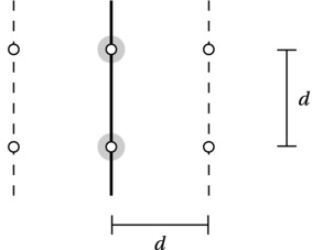
Figure 6-7. Worst case: eight points in a vertical slice of the middle region. The size of the slice is d×2d, and each of the two middle (highlighted) points represents a pair of coincident points
We’re almost done; the only remaining problems are sorting by x- and y-coordinates. We need the x-sorting to be able to divide the problem in equal halves at each step, and we need the y-sorting to do the linear traversal while merging. We can keep two arrays, one for each sorting order. We’ll be doing the recursive division on the x array, so that’s pretty straightforward. The handling of y isn’t quite so direct but still quite simple: When dividing the data set by x, we partition the y array based on x-coordinates. When combining the data, we merge them, just like in merge sort, thus keeping the sorting while using only linear time.
Note For the algorithm to work, we much return the entire subset of points, sorted, from each recursive calls. The filtering of points too far from the midline must be done on a copy.
You can see this as a way of strengthening the induction hypothesis (as discussed in Chapter 4) in order to get the desired running time: Instead of only assuming we can find the closest points in smaller point sets, we also assume that we can get the points back sorted.
Convex Hull
Here’s another geometric problem: Imagine pounding n nails into a board and strapping a rubber band around them; the shape of the rubber band is a so-called convex hull for the points represented by the nails. It’s the smallest convex14 region containing the points, that is, a convex polygon with lines between the “outermost” of the points. See Figure 6-8 for an example.
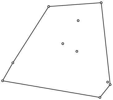
Figure 6-8. A set of points and their convex hull
By now, I’m sure you’re suspecting how we’ll be solving this: Divide the point set into two equal halves along the x-axis and solve them recursively. The only part remaining is the linear-time combination of the two solutions. Figure 6-9 hints at what we need: We must find the upper and lower common tangents. (That they’re tangents basically means that the angles they form with the preceding and following line segments should curve inward.)
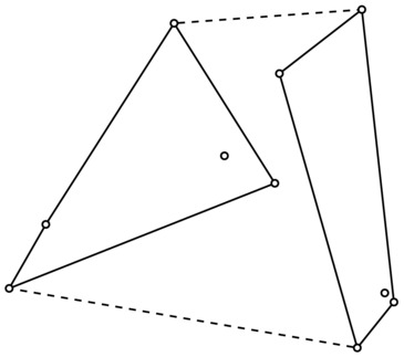
Figure 6-9. Combining two smaller convex hull by finding upper and lower common tangents (dashed)
Without going into implementation details, assume that you can check whether a line is an upper tangent for either half. (The lower part works in a similar manner.) You can then start with the rightmost point of the left half and the leftmost point of the right half. As long as the line between your points is not an upper tangent for the left part, you move to the next point along the subhull, counterclockwise. Then you do the same for the right half. You may have to do this more than once. Once the top is fixed, you repeat the procedure for the lower tangent. Finally, you remove the line segments that now fall between the tangents, and you’re done.
HOW FAST CAN WE FIND A CONVEX HULL?
The divide-and-conquer solution has a running time of O(n lgn). There are lots of algorithms for finding convex hulls, some asymptotically faster, with running times as low as O(n lgh), where h is the number of points on the hull. In the worst case, of course, all objects will fall on the hull, and we’re back to Θ(n lgn). In fact, this is the best time possible, in the worst case—but how can we know that?
We can use the idea from Chapter 4, where we show hardness through reduction. We already know from the discussion earlier in this chapter that sorting real numbers is Ω(n lgn), in the worst case. This is independent of what algorithm you use; you simply can’t do better. It’s impossible.
Now, observe that sorting can be reduced to the convex hull problem. If you want to sort n real numbers, you simply use the numbers as x-coordinates and add y-coordinates to them that place them on a gentle curve. For example, you could have y = x2. If you then find a convex hull for this point set, the values will lie in sorted order on it, and you can find the sorting by traversing its edges. This reduction will in itself take only linear time.
Imagine, for a moment, that you have a convex hull algorithm that is better than loglinear. By using the linear reduction, you subsequently have a sorting algorithm that is better than loglinear. But that’s impossible! In other words, because there exists a simple (here, linear) reduction from sorting to finding a convex hull, the latter problem is at least as hard as the former. So ... loglinear is the best we can do.
Greatest Slice
Here’s the last example: You have a sequence A containing real numbers, and you want to find a slice (or segment) A[i:j] so that sum(A[i:j]) is maximized. You can’t just pick the entire sequence, because there may be negative numbers in there as well.15 This problem is sometimes presented in the context of stock trading—the sequence contains changes in stock prices, and you want to find the interval that will give you the greatest profit. Of course, this presentation is a bit flawed, because it requires you to know all the movement of the stock beforehand.
An obvious solution would be something like the following (where n=len(A)):
result = max((A[i:j] for i in range(n) for j in range(i+1,n+1)), key=sum)
The two for clauses in the generator expression simply step through every legal start and end point, and we then take the maximum, using the sum of A[i:j] as the criterion (key). This solution might score “cleverness” points for its concision, but it’s not really that clever. It’s a naïve brute-force solution, and its running time is cubic (that is, Θ(n3))! In other words, it’s really bad.
It might not be immediately apparent how we can avoid the two explicit for loops, but let’s start by trying to avoid the one hiding in sum. One way to do this would be to consider all intervals of length k in one iteration, then move to k+1, and so on. This would still give us a quadratic number of intervals to check, but we could use a trick to make the scan cost linear: We calculate the sum for the first interval as normal, but each time the interval is shifted one position to the right, we simply subtract the element that now falls outside it, and we add the new element:
best = A[0]
for size in range(1,n+1):
    cur = sum(A[:size])
    for i in range(n-size):
        cur += A[i+size] - A[i]
        best = max(best, cur)
That’s not a lot better, but at least now we’re down to a quadratic running time. There’s no reason to quit here, though.
Let’s see what a little divide and conquer can buy us. When you know what to look for, the algorithm—or at least a rough outline—almost writes itself: Divide the sequence in two, find the greatest slice in either half (recursively), and then see whether there’s a greater one straddling the middle (as in the closest point example). In other words, the only thing that requires creative problem solving is finding the greatest slice straddling the middle. We can reduce that even further—that slice will necessarily consist of the greatest slice extending from the middle to the left and the greatest slice extending from the middle to the right. We can find these separately, in linear time, by simply traversing and summing from the middle in either direction.
Thus, we have our loglinear solution to the problem. Before leaving it entirely, though, I’ll point out that there is, in fact, a linear solution as well; see Exercise 6-18.
REALLY DIVIDING THE WORK: MULTIPROCESSING
The purpose of the divide-and-conquer design method is to balance the workload so that each recursive call takes as little time as possible. You could go even further, though, and ship the work out to separate processors (or cores). If you have a huge number of processors to use, you could then, in theory, do nifty things such as finding the maximum or sum of a sequence in logarithmic time. (Do you see how?)
In a more realistic scenario, you might not have an unlimited supply of processors at your disposal, but if you’d like to exploit the power of those you have, the multiprocessing module can be your friend. Parallel programming is commonly done using parallel (operating system) threads. Although Python has a threading mechanism, it does not support true parallel execution. What you can do, though, is use parallel processes, which in modern operating systems are really efficient. The multiprocessing module gives you an interface that makes handling parallel processes look quite a bit like threading.
Tree Balance ... and Balancing16
If we insert random values into a binary search tree, it’s going to end up pretty balanced on average. If we’re unlucky, though, we could end up with a totally unbalanced tree, basically a linked list, like the one in Figure 6-1. Most real-world uses of search trees include some form of balancing, that is, a set of operations that reorganize the tree, to make sure it is balanced (but without destroying its search tree property, of course).
There’s a ton of different tree structures and balancing methods, but they’re generally based on two fundamental operations:
- Node splitting (and merging). Nodes are allowed to have more than two children (and more than one key), and under certain circumstances, a node can become overfull. It is then split into two nodes (potentially making its parent overfull).
- Node rotations. Here we still use binary trees, but we switch edges. If x is the parent of y, we now make y the parent of x. For this to work, x must take over one of the children of y.
This might seem a bit confusing in the abstract, but I’ll go into a bit more detail, and I’m sure you’ll see how it all works. Let’s first consider a structure called the 2-3-tree. In a plain binary tree, each node can have up to two children, and they each have a single key. In a 2-3-tree, though, we allow a node to have one or two keys and up to three children. Anything in the left subtree now has to be smaller than the smallest of the keys, and anything in the right subtree is greater than the greatest of the keys—and anything in the middle subtree must fall between the two. Figure 6-10 shows an example of the two node types of a 2-3-tree.
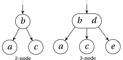
Figure 6-10. The node types in a 2-3-tree
Note The 2-3-tree is a special case of the B-tree, which forms the basis of almost all database systems, and disk-based trees used in such diverse areas as geographic information systems and image retrieval. The important extension is that B-trees can have thousands of keys (and subtrees), and each node is usually stored as a contiguous block on disk. The main motivation for the large blocks is to minimize the number of disk accesses.
Searching a 2-3-node is pretty straightforward—just a recursive traversal with pruning, like in a plain binary search tree. Insertion requires a bit of extra attention, though. As in a binary search tree, you first search for the proper leaf where the new value can be inserted. In a binary search tree, though, that will always be a None reference (that is, an empty child), where you can “append” the new node as a child of an existing one. In a 2-3-tree, though, you’ll always try to add the new value to an existing leaf. (The first value added to the tree will necessarily need to create a new node, though; that’s the same for any tree.) If there’s room in the node (that is, it’s a 2-node), you simply add the value. If not, you have three keys to consider (the two already there and your new one).
The solution is to split the node, moving the middle of the three values up to the parent. (If you’re splitting the root, you’ll have to make a new root.) If the parent is now overfull, you’ll need to split that, and so forth. The important result of this splitting behavior is that all leaves end up on the same level, meaning that the tree is fully balanced.
Now, while the idea of node splitting is relatively easy to understand, let’s stick to our even simpler binary trees for now. You see, it’s possible to use the idea of the 2-3-tree while not really implementing it as a 2-3-tree. We can simulate the whole thing using only binary nodes! There are two upsides to this: First, the structure is simpler and more consistent, and second, you get to learn about rotations (an important technique in general) without having to worry about a whole new balancing scheme!
The “simulation” I’m going to show you is called the AA-tree, after its creator, Arne Andersson.17 Among the many rotation-based balancing schemes, the AA-tree really stands out in its simplicity (though there’s still quite a bit to wrap your head around, if you’re new to this kind of thing). The AA-tree is a binary tree, so we need to have a look at how to simulate the 3-nodes we’ll be using to get balance. You can see how this works in Figure 6-11.
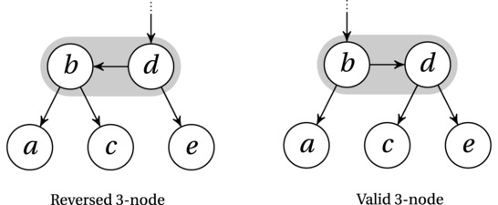
Figure 6-11. Two simulated 3-nodes (highlighted) in an AA-tree. Note that the one on the left is reversed and must be repaired
This figure shows you several things at once. First, you get an idea of how a 3-node is simulated: You simply link up two nodes to act as a single pseudonode (as highlighted). Second, the figure illustrates the idea of level. Each node is assigned a level (a number), with the level of all leaves being 1. When we pretend that two nodes form a 3-node, we simply give them the same level, as shown by the vertical placement in the figure. Third, the edge “inside” a 3-node (called a horizontal edge) can point only to the right. That means that the leftmost subfigure illustrates an illegal node, which must be repaired, using a right rotation: Make c the left child of d and d the right child of b, and finally, make d’s old parent the parent of b instead. Presto! You’ve got the rightmost subfigure (which is valid). In other words, the edge to the middle child and the horizontal edge switch places. This operation is called skew.
There is one other form of illegal situation that can occur and that must be fixed with rotations: an overfull pseudonode (that is, a 4-node). This is shown in Figure 6-12. Here we have three nodes chained on the same level (c, e, and f). We want to simulate a split, where the middle key (e) would be moved up to the parent (a), as in a 2-3-tree. In this case, that’s as simple as rotating c and e, using a left rotation. This is basically just the opposite of what we did in Figure 6-11. In other words, we move the child pointer of c down from e to d, and we move the child pointer of e up from d to c. Finally, we move the child pointer of a from c to e. To later remember that a and e now form a new 3-node, we increment the level of e (see Figure 6-12). This operation is called (naturally enough) split.
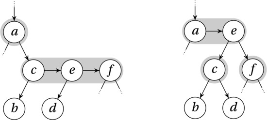
Figure 6-12. An overfull pseudonode, and the result of the repairing left rotation (swapping the edges (e,d) and (c,e)), as well as making e the new child of a
You insert a node into an AA-tree just like you would in a standard, unbalanced binary tree; the only difference is that you perform some cleanup afterward (using skew and split). The full code can be found in Listing 6-6. As you can see, the cleanup (one call to skew and one to split) is performed as part of the backtracking in the recursion—so nodes are repaired on the path back up to the root. How does that work, really?
The operations further down along the path can really do only one thing that will affect us: They can put another node into “our” current simulated node. At the leaf level, this happens whenever we add a node, because they all have level 1. If the current node is further up in the tree, we can get another node in our current (simulated) node if one has been moved up during a split. Either way, this node that is now suddenly on our level can be either a left child or a right child. If it’s a left child, we skew (do a right rotation), and we’ve gotten rid of the problem. If it’s a right child, it’s not a problem to begin with. However, if it’s a right grandchild, we have an overfull node, so we do a split (a left rotation) and promote the middle node of our simulated 4-node up to the parent’s level.
This is all pretty tricky to describe in words—I hope the code is clear enough that you’ll understand what’s going on. (It might take some time and head-scratching, though.)
Listing 6-6. The Binary Search Tree, Now with AA-Tree Balancing
class Node:
    lft = None
    rgt = None
    lvl = 1                                     # We've added a level...
    def __init__(self, key, val):
        self.key = key
        self.val = val

def skew(node):                                 # Basically a right rotation
    if None in [node, node.lft]: return node    # No need for a skew
    if node.lft.lvl != node.lvl: return node    # Still no need
    lft = node.lft                              # The 3 steps of the rotation
    node.lft = lft.rgt
    lft.rgt = node
    return lft                                  # Switch pointer from parent

def split(node):                                # Left rotation & level incr.
    if None in [node, node.rgt, node.rgt.rgt]: return node
    if node.rgt.rgt.lvl != node.lvl: return node
    rgt = node.rgt
    node.rgt = rgt.lft
    rgt.lft = node
    rgt.lvl += 1                                # This has moved up
    return rgt                                  # This should be pointed to

def insert(node, key, val):
    if node is None: return Node(key, val)
    if node.key == key: node.val = val
    elif key < node.key:
        node.lft = insert(node.lft, key, val)
    else:
        node.rgt = insert(node.rgt, key, val)
    node = skew(node)                           # In case it's backward
    node = split(node)                          # In case it's overfull
    return node
Can we be sure that the AA-tree will be balanced? Indeed we can, because it faithfully simulates the 2-3-tree (with the level property representing actual tree levels in the 2-3-tree). The fact that there’s an extra edge inside the simulated 3-nodes can no more than double any search path, so the asymptotic search time is still logarithmic.
BLACK BOX: BINARY HEAPS, HEAPQ, AND HEAPSORT
A priority queue is a generalization of the LIFO and FIFO queues discussed in Chapter 5. Instead of basing the order only on when an item is added, each item receives a priority, and you always retrieve the remaining item with the lowest priority. (You could also use maximum priority, but you normally can’t have both in the same structure.) This kind of functionality is important as a component of several algorithms, such as Prim’s, for finding minimum spanning trees (Chapter 7), or Dijkstra’s, for finding shortest paths (Chapter 9). There are many ways of implementing a priority queue, but probably the most common data structure used for this purpose is the binary heap. (There are other kinds of heaps, but the unqualified term heap normally refers to binary heaps.)
Binary heaps are complete binary trees. That means they are as balanced as they can get, with each level of the tree filled up, except (possibly) the lowest level, which is filled as far as possible from the left. Arguably the most important aspect of their structure, though, is the so-called heap property: The value of every parent is smaller than those of both children. (This holds for a minimum heap; for a maximum heap, each parent is greater.) As a consequence, the root has the smallest value in the heap. The property is similar to that of search trees but not quite the same, and it turns out that the heap property is much easier to maintain without sacrificing the balance of the tree. You never modify the structure of the tree by splitting or rotating nodes in a heap. You only ever need to swap parent and child nodes to restore the heap property. For example, to “repair” the root of a subtree (which is too big), you simply swap it with its smallest child and repair that subtree recursively (as needed).
The heapq module contains an efficient heap implementation that represents its heaps in lists, using a common “encoding”: If a is a heap, the children of a[i] are found in a[2*i+1] and a[2*i+2]. This means that the root (the smallest element) is always found in a[0]. You can build a heap from scratch, using the heappush and heappop functions. You might also start out with a list that contains lots of values, and you’d like to make it into a heap. In that case, you can use the heapify function.18 It basically repairs every subtree root, starting at the bottom right, moving left and up. (In fact, by skipping the leaves, it needs only work on the left half of the array.) The resulting running time is linear (see Exercise 6-9). If your list is sorted, it’s already a valid heap, so you can just leave it alone.
Here’s an example of building a heap piece by piece:
>>> from heapq import heappush, heappop
>>> from random import randrange
>>> Q = []
>>> for i in range(10):
... heappush(Q, randrange(100))
...
>>> Q
[15, 20, 56, 21, 62, 87, 67, 74, 50, 74]
>>> [heappop(Q) for i in range(10)]
[15, 20, 21, 50, 56, 62, 67, 74, 74, 87]
Just like bisect, the heapq module is implemented in C, but it used to be a plain Python module. For example, here is the code (from Python 2.3) for the function that moves an object down until it’s smaller than both of its children (again, with my comments):
def sift_up(heap, startpos, pos):
newitem = heap[pos] # The item we're sifting up
while pos > startpos: # Don't go beyond the root
parentpos = (pos - 1) >>1 # The same as (pos - 1) // 2
parent = heap[parentpos] # Who's your daddy?
if parent <= newitem: break # Valid parent found
heap[pos] = parent # Otherwise: copy parent down
pos = parentpos # Next candidate position
heap[pos] = newitem # Place the item in its spot
Note that the original function was called _siftdown because it’s sifting the value down in the list. I prefer to think of it as sifting it up in the implicit tree structure of the heap, though. Note also that, just like bisect_right, the implementation uses a loop rather than recursion.
In addition to heappop, there is heapreplace, which will pop the smallest item and insert a new element at the same time, which is a bit more efficient than a heappop followed by a heappush. The heappop operation returns the root (the first element). To maintain the shape of the heap, the last item is moved to the root position, and from there it is swapped downward (in each step, with its smallest child) until it is smaller than both its children. The heappush operation is just the reverse: The new element is appended to the list and is repeatedly swapped with its parent until it is greater than its parent. Both of these operations are logarithmic (also in the worst case, because the heap is guaranteed to be balanced).
Finally, the module has (since version 2.6) the utility functions merge, nlargest, and nsmallest for merging sorted inputs and finding the n largest and smallest items in an iterable, respectively. The latter two functions, unlike the others in the module, take the same kind of key argument as list.sort. You can simulate this in the other functions with the DSU pattern, as mentioned in the sidebar on bisect.
Although you would probably never use them that way in Python, the heap operations can also form a simple, efficient, and asymptotically optimal sorting algorithm called heapsort. It is normally implemented using a max-heap and works by first performing heapify on a sequence, then repeatedly popping off the root (as in heappop), and finally placing it in the now empty last slot. Gradually, as the heap shrinks, the original array is filled from the right with the largest element, the second largest, and so forth. In other words, heap sort is basically selection sort where a heap is used to implement the selection. Because the initialization is linear and each of the n selections is logarithmic, the running time is loglinear, that is, optimal.
Summary
The algorithm design strategy of divide and conquer involves a decomposition of a problem into roughly equal-sized subproblems, solving the subproblems (often by recursion), and combining the results. The main reason this is useful it that the workload is balanced, typically taking you from a quadratic to a loglinear running time. Important examples of this behavior include merge sort and quicksort, as well as algorithms for finding the closest pair or the convex hull of a point set. In some cases (such as when searching a sorted sequence or selecting the median element), all but one of the subproblems can be pruned, resulting in a traversal from root to leaf in the subproblem graph, yielding even more efficient algorithms.
The subproblem structure can also be represented explicitly, as it is in binary search trees. Each node in a search tree is greater than the descendants in its left subtree but less than those in its right subtree. This means that a binary search can be implemented as a traversal from the root. Simply inserting random values haphazardly will, on average, yield a tree that is balanced enough (resulting in logarithmic search times), but it is also possible to balance the tree, using node splitting or rotations, to guarantee logarithmic running times in the worst case.
If You’re Curious ...
If you like bisection, you should look up interpolation search, which for uniformly distributed data has an average-case running time of O(lg lg n). For implementing sets (that is, efficient membership checking) other than sorted sequences, search trees and hash tables, you could have a look at Bloom filters. If you like search trees and related structures, there are lots of them out there. You could find tons of different balancing mechanisms (red black trees, AVL-trees, splay trees), some of them randomized (treaps), and some of them only abstractly representing trees (skip lists). There are also whole families of specialized tree structures for indexing multidimensional coordinates (so-called spatial access methods) and distances (metric access methods). Other trees structures to check out are interval trees, quadtrees, and octtrees.
Exercises
6-1. Write a Python program that implements the solution to the skyline problem.
6-2. Binary search divides the sequence into two approximately equal parts in each recursive step. Consider ternary search, which divides the sequence into three parts. What would its asymptotic complexity be? What can you say about the number of comparisons in binary and ternary search?
6-3. What is the point of multiway search trees, as opposed to binary search trees?
6-4. How could you extract all keys from a binary search tree in sorted order, in linear time?
6-5. How would you delete a node from a binary search tree?
6-6. Let’s say you insert n random values into an initially empty binary search tree. What would, on average, be the depth of the leftmost (that is, smallest) node?
6-7. In a min-heap, when moving a large node downward, you always switch places with the smallest child. Why is that important?
6-8. How (or why) does the heap encoding work?
6-9. Why is the operation of building a heap linear?
6-10. Why wouldn’t you just use a balanced binary search tree instead of a heap?
6-11. Write a version of partition that partitions the elements in place (that is, moving them around in the original sequence). Can you make it faster than the one in Listing 6-3?
6-12. Rewrite quicksort to sort elements in place, using the in-place partition from Exercise 6-11.
6-13. Let’s say you rewrote select to choose the pivot using, for example, random.choice. What difference would that make? (Note that the same strategy can be used to create a randomized quicksort.)
6-14. Implement a version of quicksort that uses a key function, just like list.sort.
6-15. Show that a square of side d can hold at most four points that are all at least a distance of d apart.
6-16. In the divide-and-conquer solution to the closest pair problem, you can get away with examining at most the next seven points in the mid-region points, sorted by y-coordinate. Show how you could quite easily reduce this number to five.
6-17. The element uniqueness problem is to determine whether all elements of a sequence are unique. This problem has a proven loglinear lower bound in the worst case for real numbers. Show that this means the closest pair problem also has a loglinear lower bound in the worst case.
6-18. How could you solve the greatest slice problem in linear time?
References
Andersson, A. (1993). Balanced search trees made simple. In Proceedings of the Workshop on Algorithms and Data Structures (WADS), pages 60-71.
Bayer, R. (1971). Binary B-trees for virtual memory. In Proceedings of the ACM SIGFIDET Workshop on Data Description, Access and Control, pages 219-235.
Blum, M., Floyd, R. W., Pratt, V., Rivest, R. L., and Tarjan, R. E. (1973). Time bounds for selection. Journal of Computer and System Sciences, 7(4):448-461.
de Berg, M., Cheong, O., van Kreveld, M., and Overmars, M. (2008). Computational Geometry: Algorithms and Applications, third edition. Springer.
__________________
1Note that some authors use the conquer term for the base case of the recursion, yielding the slightly different ordering: divide, conquer, and combine.
2Described by Udi Manber in his Introduction to Algorithms (see “References” in Chapter 4).
3For example, in the skyline problem, you would probably want to split the base case element (L,H,R) into two pairs, (L,H) and (R,H), so the combine function can build a sequence of points.
4Actually, more flexible may not be entirely correct. There are many objects (such as complex numbers) that can be hashed but that cannot be compared for size.
5In statistics, the median is also defined for sequences of even length. It is then the average of the two middle elements. That’s not an issue we worry about here.
6In theory, we could use the guaranteed linear version of select to find the median and use that as a pivot. That’s not something likely to happen in practice, though.
7Timsort is, in fact, also used in Java SE 7, for sorting arrays.
8See, for example, the file listsort.txt in the source code (or online, http://svn.python.org/projects/python/trunk/Objects/listsort.txt).
9You can find the actual C code at http://svn.python.org/projects/python/trunk/Objects/listobject.c.
10See https://bitbucket.org/pypy/pypy/src/default/rpython/rlib/listsort.py.
11Real numbers usually aren’t all that arbitrary, of course. As long as your numbers use a fixed number of bits, you can use radix sort (mentioned in Chapter 4) and sort the values in linear time.
12I think that’s so cool, I wanted to add an exclamation mark after the sentence ... but I guess that might have been a bit confusing, given the subject matter.
13Actually, the approximation isn’t asymptotic in nature. If you want the details, you’ll find them in any good mathematics reference.
14A region is convex if you can draw a line between any two points inside it, and the line stays inside the region.
15I’m still assuming that we want a nonempty interval. If it turns out to have a negative sum, you could always use an empty interval instead.
16This section is a bit hard and is not essential in order to understand the rest of the book. Feel free to skim it or even skip it entirely. You might want to read the “Black Box” sidebar on binary heaps, heapq, and heapsort, though, later in the section.
17The AA-tree is, in a way, a version of the BB-tree, or the binary B-tree, which was introduced by Rudolph Bayer in 1971 as a binary representation of the 2-3-tree.
18It is quite common to call this operation build-heap and to reserve the name heapify for the operation that repairs a single node. Thus, build-heap runs heapify on all nodes but the leaves.