Table of Contents for
Python Algorithms: Mastering Basic Algorithms in the Python Language, Second Edition
 Python Algorithms: Mastering Basic Algorithms in the Python Language, Second Edition
Published by
Apress, 2015
Python Algorithms: Mastering Basic Algorithms in the Python Language, Second Edition
Published by
Apress, 2015
- Cover
- Title
- Copyright
- Dedication
- Contents at a Glance
- Contents
- About the Author
- About the Technical Reviewer
- Acknowledgments
- Preface
- Chapter 1: Introduction
- Chapter 2: The Basics
- Chapter 3: Counting 101
- Chapter 4: Induction and Recursion … and Reduction
- Chapter 5: Traversal: The Skeleton Key of Algorithmics
- Chapter 6: Divide, Combine, and Conquer
- Chapter 7: Greed Is Good? Prove It!
- Chapter 8: Tangled Dependencies and Memoization
- Chapter 9: From A to B with Edsger and Friends
- Chapter 10: Matchings, Cuts, and Flows
- Chapter 11: Hard Problems and (Limited) Sloppiness
- Appendix A: Pedal to the Metal: Accelerating Python
- Appendix B: List of Problems and Algorithms
- Appendix C: Graph Terminology
- Appendix D: Hints for Exercises
- Index

Matchings, Cuts, and Flows
A joyful life is an individual creation that cannot be copied from a recipe.
— Mihaly Csikszentmihalyi, Flow: The Psychology of Optimal Experience
While the previous chapter gave you several algorithms for a single problem, this chapter describes a single algorithm with many variations and applications. The core problem is that of finding maximum flow in a network, and the main solution strategy I’ll be using is the augmenting path method of Ford and Fulkerson. Before tackling the full problem, I’ll guide you through two simpler problems, which are basically special cases (they’re easily reduced to maximum flow). These problems, bipartite matching and disjoint paths, have many applications themselves and can be solved by more specialized algorithms. You’ll also see that the max-flow problem has a dual, the min-cut problem, which means that you’ll automatically solve both problems at the same time. The min-cut problem has several interesting applications that seem very different from those of max-flow, even if they are really closely related. Finally, I’ll give you some pointers on one way of extending the max-flow problem, by adding costs, and looking for the cheapest of the maximum flows, paving the way for applications such as min-cost bipartite matching.
The max-flow problem and its variations have almost endless applications. Douglas B. West, in his book Introduction to Graph Theory (see “References” in Chapter 2), gives some rather obvious ones, such as determining the total capacities of road and communication networks, or even working with currents in electrical circuits. Kleinberg and Tardos (see “References” in Chapter 1) explain how to apply the formalism to survey design, airline scheduling, image segmentation, project selection, baseball elimination, and assigning doctors to holidays. Ahuja, Magnanti, and Orlin have written one of the most thorough books on the subject and cover well over 100 applications in such diverse areas as engineering, manufacturing, scheduling, management, medicine, defense, communication, public policy, mathematics, and transportation. Although the algorithms apply to graphs, these application need not be all that graphlike at all. For example, who’d think of image segmentation as a graph problem? I’ll walk you through some of these applications in the unsurprisingly named section “Some Applications” later in the chapter. If you’re curious about how the techniques can be used, you might want to take a quick glance at that section before reading on.
The general idea that runs through this chapter is that we’re trying to get the most out of a network, moving from one side to the other, pushing through as much of we can of some kind of substance—be it edges of a bipartite matching, edge-disjoint paths, or units of flow. This is a bit different from the cautious graph exploration in the previous chapter. The basic approach of incremental improvement is still here, though. We repeatedly find ways of improving our solutions slightly, until it can’t get any better. You’ll see that the idea of canceling is key—that we may need to remove parts of a previous solution in order to make it better overall.
 Note I’m using the labeling approach due to Ford and Fulkerson for the implementations in this chapter. Another perspective on the search for augmenting paths is that we’re traversing a residual network. This idea is explained in the sidebar “Residual Networks” later in the chapter.
Bipartite Matching
I’ve already exposed you to the idea of bipartite matching, both in the form of the grumpy moviegoers in Chapter 4 and in the stable marriage problem in Chapter 7. In general, a matching for a graph is a node-disjoint subset of the edges. That is, we select some of the edges in such a way that no two edges share a node. This means that each edge matches two pairs—hence the name. A special kind of matching applies to bipartite graphs, graphs that can be partitioned into two independent node sets (subgraphs without edges), such as the graph in Figure 10-1. This is exactly the kind of matching we’ve been working with in the moviegoer and marriage problems, and it’s much easier to deal with than the general kind. When we talk about bipartite matching, we usually want a maximum matching, one that consists of a maximum number of edges. This means, if possible, we’d like a perfect matching, one where all nodes are matched. This is a simple problem but one that can easily occur in real life. Let’s say, for example, you’re assigning people to projects, and the graph represents who’d like to work on what. A perfect matching would please everyone.1
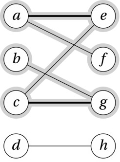
Figure 10-1. A bipartite graph with a (non-maximal) matching (heavy edges) and an augmenting path from b to f (highlighted)
We can continue to use the metaphor from the stable marriage problem—we’ll just drop the stability and try to get everyone matched with someone they can accept. To visualize what’s going on, let’s say each man has an engagement ring. What we want is then to have each man give his ring to one of the women so that no woman has more than one ring. Or, if that’s not possible, we want to move as many rings as possible from the men to the women, still prohibiting any woman from keeping more than one. As always, to solve this, we start looking for some form of reduction or inductive step. An obvious idea would be to somehow identify a pair of lovers destined to be together, thereby reducing the number of pairs we need to worry about. However, it’s not so easy to guarantee that any single pair is part of a maximum matching, unless, for example, it’s totally isolated, like d and h in Figure 10-1.
An approach that fits better in this case is iterative improvement, as discussed in Chapter 4. This is closely related to the use of relaxation in Chapter 9, in that we’ll improve our solution step by step, until we can’t improve it anymore. We also have to make sure that the only reason the improvement stops is that the solution is optimal—but I’ll get back to that. Let’s start by finding some step by step improvement scheme. Let’s say that in each round we try to move one additional ring from the men to the women. If we’re lucky, this would give us the solution straightaway—that is, if each man gives the ring to the woman he’d be matched to in the best solution. We can’t let any romantic tendencies cloud our vision here, though. Chances are this approach won’t work quite that smoothly. Consider, once again, the graph in Figure 10-1. Let’s say that in our first two iterations, a gives a ring to e, and c gives one to g. This gives us a tentative matching consisting of two pairs (indicated by the heavy black edges). Now we turn to b. What is he to do?
Let’s follow a strategy somewhat similar to the Gale-Shapley algorithm mentioned in Chapter 7, where the women can change their minds when approached by a new suitor. In fact, let’s mandate that they always do. So when b asks g, she returns her current ring to c, accepting the one from b. In other words, she cancels her engagement to c. (This idea of canceling is crucial to all the algorithms in this chapter.) But now c is single, and if we are to ensure that the iteration does indeed lead to improvement, we can’t accept this new situation. We immediately look around for a new mate for c, in this case e. But if c passes his returned ring to e, she has to cancel her engagement to a, returning his ring. He in turn passes this on to f, and we’re done. After this single zigzag swapping session, rings have been passed back and forth along the highlighted edges. Also, we now have increased the number of couples from two to three (a + f, b + g, and c + e).
We can, in fact, extract a general method from this ad hoc procedure. First, we need to find one unmatched man. (If we can’t, we’re done.) We then need to find some alternating sequence of engagements and cancellations so that we end with an engagement. If we can find that, we know that there must have been one more engagement than there were cancellations, increasing the number of pairs by one. We just keep finding such zigzags for as long as we can.
The zigzags we’re looking for are paths that go from an unmatched node on the left side to an unmatched node on the right side. Following the logic of the engagement rings, we see that the path can only move to the right across an edge that is not already in the matching (a proposal), and it can only move left across one that is in the matching (a cancellation). Such a path (like the one highlighted in Figure 10-1) is called an augmenting path, because it augments our solution (that is, it increments the engagement count), and we can find augmenting paths by traversal. We just need to be sure we follow the rules—we can’t follow matched edges to the right or unmatched edges to the left.
What’s left is ensuring that we can indeed find such augmenting paths as long as there is room for improvement. Although this seems plausible enough, it’s not immediately obvious why it must be so. What we want to show is that if there is room for improvement, we can find an augmenting path. That means that we have a current match M and that there is some greater matching M’ that we haven’t found yet. Now consider the edges in the symmetric difference between these two—that is, the edges that are in either one but not in both. Let’s call the edges in M red and the ones in M’ green.
This jumble of red and green edges would actually have some useful structure. For example, we know that each node would be incident to at most two edges, one of each color (because it couldn’t have two edges from the same matching). This means that we’d have one or more connected components, each of which was a zigzagging path or cycle of alternating color. Because M’ is bigger than M, we must have at least one component with more green than red edges, and the only way that could happen would be in a path—an odd-length one that started and ended with a green edge.
Do you see it yet? Exactly! This green-red-…-green path would be an augmenting path. It has odd length, so one end would be on the male side and one on the female. And the first and last edges were green, meaning they were not part of our original matching, so we’re free to start augmenting. (This is essentially my take on what’s known as Berge’s lemma.)
When it comes to implementing this strategy, there is a lot of room for creativity. One possible implementation is shown in Listing 10-1. The code for the tr function can be found in Listing 5-10. The parameters X and Y are collections (iterable objects) of nodes, representing the bipartition of the graph G. The running time might not be obvious, because edges are switched on and off during execution, but we do know that one pair is added to the matching in each iteration, so the number of iterations is O(n), for n nodes. Assuming m edges, the search for an augmenting path is basically a traversal of a connected component, which is O(m). In total, then, the running time is O(nm).
Listing 10-1. Finding a Maximum Bipartite Matching Using Augmenting Paths
from itertools import chain

def match(G, X, Y):                             # Maximum bipartite matching
    H = tr(G)                                   # The transposed graph
    S, T, M = set(X), set(Y), set()             # Unmatched left/right + match
    while S:                                    # Still unmatched on the left?
        s = S.pop()                             # Get one
        Q, P = {s}, {}                          # Start a traversal from it
        while Q:                                # Discovered, unvisited
            u = Q.pop()                         # Visit one
            if u in T:                          # Finished augmenting path?
                T.remove(u)                     # u is now matched
                break                           # and our traversal is done
            forw = (v for v in G[u] if (u,v) not in M)  # Possible new edges
            back = (v for v in H[u] if (v,u) in M)      # Cancellations
            for v in chain(forw, back):         # Along out- and in-edges
                if v in P: continue             # Already visited? Ignore
                P[v] = u                        # Traversal predecessor
                Q.add(v)                        # New node discovered
        while u != s:                           # Augment: Backtrack to s
            u, v = P[u], u                      # Shift one step
            if v in G[u]:                       # Forward edge?
                M.add((u,v))                    # New edge
            else:                               # Backward edge?
                M.remove((v,u))                 # Cancellation
    return M                                    # Matching -- a set of edges
Note König’s theorem states that for bipartite graph, the dual of the maximum matching problem is the minimum vertex cover problem. In other words, the problems are equivalent.
Disjoint Paths
The augmenting path method for finding matchings can also be used for more general problems. The simplest generalization may be to count edge-disjoint paths instead of edges.2 Edge-disjoint paths can share nodes but not edges. In this more general setting, we no longer need to restrict ourselves to bipartite graphs. When we allow general directed graphs, however, we can freely specify where the paths are to start and end. The easiest (and most common) solution is to specify two special nodes, s and t, called the source and the sink. (Such a graph is often called an s-t graph, or an s-t-network.) We then require all paths to start in s and end in t (implicitly allowing the paths to share these two nodes). An important application of this problem is determining the edge connectivity of a network—how many edges can be removed (or “fail”) before the graph is disconnected (or, in this case, before s cannot reach t)?
Another application is finding communication paths on a multicore CPU. You may have lots of cores laid out in two dimensions, and because of the way communication works, it can be impossible to route two communication channels through the same switching points. In these cases, finding a set of disjoint paths is critical. Note that these paths would probably be more naturally modeled as vertex-disjoint, rather than edge-disjoint. See Exercise 10-2 for more. Also, as long as you need to pair each source core with a specific sink core, you have a version of what’s called the multicommodity flow problem, which isn’t dealt with here. (See “If You’re Curious …” for some pointers.)
You could deal with multiple sources and sinks directly in the algorithm, just like in Listing 10-1. If each of these sources and sinks can be involved only in a single path and you don’t care which source is paired with which sink, it can be easier to reduce the problem to the single-source, single-sink case. You do this by adding s and t as new nodes and introduce edges from s to all of your sources and from all your sinks to t. The number of paths will be the same, and reconstructing the paths you were looking for requires only snipping off s and t again. This reduction, in fact, makes the maximum matching problem a special case of the disjoint paths problem. As you’ll see, the algorithms for solving the problems are also very similar.
Instead of thinking about complete paths, it would be useful to be able to look at smaller parts of the problem in isolation. We can do that by introducing two rules:
- The number of paths going into any node except s or t must equal the number of paths going out of that node.
- At most one path can go through any given edge.
Given these restrictions, we can use traversal to find paths from s to t. At some point, we can’t find any more paths without overlapping with some of those we already have. Once again, though, we can use the augmenting path idea from the previous section. See, for example, Figure 10-2. A first round of traversal has established one path from s to t via c and b. Now, any further progress seems blocked by this path—but the augmenting path idea lets us improve the solution by canceling the edge from c to b.
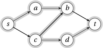
Figure 10-2. An s-t network with one path found (heavy edges) and one augmenting path (highlighted)
The principle of canceling works just like in bipartite matching. As we search for an augmenting path, we move from s to a and then to b. There, we’re blocked by the edge bt. The problem at this point is that b has two incoming paths from a and c but only one outgoing path. By canceling the edge cb, we’ve solved the problem for b, but now there’s a problem at c. This is the same kind of cascade effect we saw for the bipartite matching. In this case, c has an incoming path from s, but no outgoing path—we need to find somewhere for the path to go. We do that by continuing our path via d to t, as shown by the highlights in Figure 10-2.
If you either add an incoming edge or cancel an outgoing one at some node u, that node will be overcrowded. It will have more paths entering than leaving, which isn’t allowed. You can fix this either by adding an outgoing edge or by canceling an incoming one. All in all, this works out to finding a path from s, following unused edges in their direction and used ones against their direction. Any time you can find such an augmenting path, you will also have discovered an additional disjoint path.
Listing 10-2 shows code for implementing this algorithm. As before, the code for the tr function can be found in Listing 5-10.
Listing 10-2. Counting Edge-Disjoint Paths Using Labeling Traversal to Find Augmenting Paths
from itertools import chain

def paths(G, s, t):                             # Edge-disjoint path count
    H, M, count = tr(G), set(), 0               # Transpose, matching, result
    while True:                                 # Until the function returns
        Q, P = {s}, {}                          # Traversal queue + tree
        while Q:                                # Discovered, unvisited
            u = Q.pop()                         # Get one
            if u == t:                          # Augmenting path!
                count += 1                      # That means one more path
                break                           # End the traversal
            forw = (v for v in G[u] if (u,v) not in M)  # Possible new edges
            back = (v for v in H[u] if (v,u) in M)      # Cancellations
            for v in chain(forw, back):         # Along out- and in-edges
                if v in P: continue             # Already visited? Ignore
                P[v] = u                        # Traversal predecessor
                Q.add(v)                        # New node discovered
        else:                                   # Didn't reach t?
            return count                        # We're done
        while u != s:                           # Augment: Backtrack to s
            u, v = P[u], u                      # Shift one step
            if v in G[u]:                       # Forward edge?
                M.add((u,v))                    # New edge
            else:                               # Backward edge?
                M.remove((v,u))                 # Cancellation
To make sure we’ve solved the problem, we still need to prove the converse, though—that there always will be an augmenting path as long as there is room for improvement. The easiest way of showing this is by using the idea of connectivity: how many edges must we remove to separate s from t (so that no path goes from s to t)? Any such set represents an s-t cut, a partitioning into two sets S and T, where S contains s and T contains t. We call the edges going from S to T a directed edge separator. We can then show that the following three statements are equivalent:
- We have found k disjoint paths and there is an edge separator of size k.
- We have found the maximum number of disjoint paths.
- There are no augmenting paths.
What we primarily want to show is that the last two statements are equivalent, but sometimes it’s easier to go via a third statement, such as the first one in this case.
It’s pretty easy to see that the first implies the second. Let’s call the separator F. Any s-t path must have at least one edge in F, which means that the size of F is at least as great as the number of disjoint s-t paths. If the size of the separator is the same as the number of disjoint paths we’ve found, clearly we’ve reached the maximum.
Showing that the second statement implies the third is easily done by contradiction. Assume there is no room for improvement but that we still have an augmenting path. As discussed, this augmenting path could be used to improve the solution, so we have a contradiction.
The only thing left to prove is that the last statement implies the first, and this is where the whole connectivity idea pays off as a stepping stone. Imagine you’ve executed the algorithm until you’ve run out of augmenting paths. Let S be the set of nodes you reached in your last traversal, and let T be the remaining nodes. Clearly, this is an s-t cut. Consider the edges across this cut. Any forward edge from S to T must be part of one of your discovered disjoint paths. If it wasn’t, you would have followed it during your traversal. For the same reason, no edge from T to S can be part of one of the paths, because you could have canceled it, thereby reaching T. In other words, all edges across from S to T belong to your disjoint paths, and because none of the edges in the other direction do, the forward edges must all belong to a path of their own, meaning that you have k disjoint paths and a separator of size k.
This may be a bit involved, but the intuition is that if we can’t find an augmenting path, there must be a bottleneck somewhere, and we must have filled it. No matter what we do, we can’t get more paths through this bottleneck, so the algorithm must have found the answer. (This result is a version of Menger’s theorem, and it is a special case of the max-flow min-cut theorem, which you’ll see in a bit.)
What’s the running time of all this, then? Each iteration consists of a relatively straightforward traversal from s, which has a running time of O(m), for m edges. Each round gives us another disjoint path, and there are clearly at most O(m), meaning that the running time is O(m2). Exercise 10-3 asks you to show that this is a tight bound in the worst case.
Note Menger’s theorem is another example of duality: The maximum number of edge-disjoint paths from s to t is equal to the minimum cut between s and t. This is a special case of the max-flow min-cut theorem, discussed later.
Maximum Flow
This is the central problem of the chapter. It forms a generalization of both the bipartite matching and the disjoint paths, and it is the mirror image of the minimum cut problem (next section). The only difference from the disjoint path case is that instead of setting the capacity for each edge to one, we let it be an arbitrary positive number. If the capacity is a positive integer, you could think of it as the number of paths that can pass through it. More generally, the metaphor here is some form of substance flowing through the network, from the source to the sink, and the capacity represents the limit for how many units can flow through a given edge. (You can think of this as a generalization of the engagement rings that were passed back and forth in the matching.) In general, the flow itself is an assignment of a number of flow units to each unit (that is, a function or mapping from edges to numbers), while the size or magnitude of the flow is the total amount pushed through the network. (This can be found by finding the net flow out of the source, for example.) Note that although flow networks are commonly defined as directed, you could find the maximum flow in an undirected network as well (Exercise 10-4).
Let’s see how we can solve this more general case. A naïve approach would be to simply split edges, just like the naïve extension of BFS in Chapter 9 (Figure 9-3). Now, though, we want to split them lengthwise, as shown in Figure 10-3. Just like BFS with serial dummy nodes gives you a good idea of how Dijkstra’s algorithm works, our augmenting path algorithm with parallel dummy nodes is very close to how the full Ford-Fulkerson algorithm for finding maximum flow works. As in the Dijkstra case, though, the actual algorithm can take care of greater chunks of flow in one go, meaning that the dummy node approach (which lets us saturate only one unit of capacity at a time) is hopelessly inefficient.
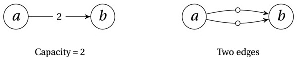
Figure 10-3. An edge capacity simulated by dummy nodes
Let’s walk through the technicalities. Just like in the zero-one case, we have two rules for how our flow interacts with edges and nodes. As you can see, they parallel the disjoint path rules closely:
- The amount of flow going into any node except s or t must equal the amount of flow going out of that node.
- At most c(e) units of flow can go through any given edge.
Here, c(e) is the capacity of edge e. Just like for the disjoint paths, we are required to follow the edge direction, so the flow back along an edge is always zero. A flow that respects our two rules is said to be feasible.
This is where you may need to take a breath and focus, though. What I’m about to say isn’t really complicated, but it can get a bit confusing. I am allowed to push flow against the direction of an edge, as long as there’s already some flow going in the right direction. Do you see how that would work? I hope the previous two sections have prepared you for this—it’s all a matter of canceling flow. If I have one unit of flow going from a to b, I can cancel that unit, in effect pushing one unit in the other direction. The net result is zero, so there is no actual flow in the wrong direction (which is totally forbidden).
This idea lets us create augmenting paths, just like before: If you add k units of flow along an incoming edge or cancel k units on an outgoing one at some node u, that node will be overflowing. It will have more flow entering than leaving, which isn’t allowed. You can fix this either by adding k units of flow along an outgoing edge or by canceling k units on an incoming one. This is exactly what you did in the zero-one case, except there k was always 1.
In Figure 10-4 two states of the same flow network are shown. In the first state, flow has been pushed along the path s-c-b-t, giving a total flow value of 2. This flow is blocking any further improvements along the forward edges. As you can see, though, the augmenting path includes a backward edge. By canceling one of the units of flow going from c to b, we can send one additional unit from c via d to t, reaching the maximum.
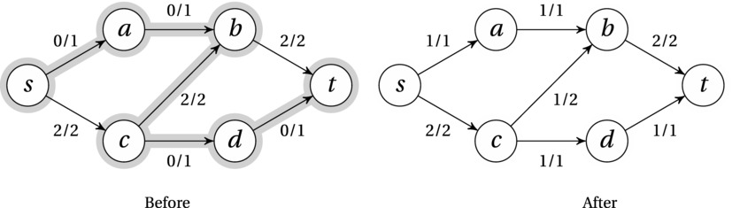
Figure 10-4. A flow network before and after augmenting via an augmenting path (highlighted)
The general Ford-Fulkerson approach, as explained in this section, does not give any running time guarantees. In fact, if irrational capacities (containing square roots or the like) are allowed, the iterative augmentation may never terminate. For actual applications, the use of irrationals may not be very realistic, but even if we restrict ourselves to limited-precision floating-point numbers, or even integers, we can still run into trouble. Consider a really simple network with source, sink, and two other nodes, u and v. Both nodes have edges from the source and to the sink, all with a capacity of k. We also have a unit-capacity edge from u to v. If we keep choosing augmenting paths that go through the edge uv, adding and canceling one unit of flow in every iteration, that would give us 2k iterations before termination.
What’s the problem with this running time? It’s pseudopolynomial—exponential in the actual problem size. We can easily crank up the capacity, and hence the running time, without using much more space. And the annoying thing is that if we had chosen the augmenting paths more cleverly (for example, just avoiding the edge uv altogether), we would have finished in two rounds, regardless of the capacity k.
Luckily, there is a solution to this problem, one that gives us a polynomial running time, no matter the capacities (even irrational ones!). The thing is, Ford-Fulkerson isn’t really a fully specified algorithm, because its traversal is completely arbitrary. If we settle on BFS as the traversal order (thereby always choosing the shortest augmenting path), we end up with what’s called the Edmonds-Karp algorithm, which is exactly the solution we’re looking for. For n nodes and m edges, Edmonds-Karp runs in O(nm2) time. That this is the case isn’t entirely obvious, though. For a thorough proof, I recommend looking up the algorithm in the book by Cormen et al. (see “References” in Chapter 1). The general idea is as follows: Each shortest augmenting path is found in O(m) time, and when we augment the flow along it, at least one edge is saturated (the flow reaches the capacity). Each time an edge is saturated, the distance from the source (along the augmenting path) must increase, and this distance is at most O(n). Because each edge can be saturated at most O(n) times, we get at O(nm) iterations and a total running time of O(nm2).
For a correctness proof for the general Ford-Fulkerson method (and therefore also the Edmonds-Karp algorithm), see the next section, on minimum cuts. That correctness proof does assume termination, though, which is guaranteed if you avoid irrational capacities or if you simply use the Edmonds-Karp algorithm (which has a deterministic running time).
One augmentation traversal, based on BFS, is given in Listing 10-3. An implementation of the full Ford-Fulkerson method is shown in Listing 10-4. For simplicity, it is assumed that s and t are different nodes. By default, the implementation uses the BFS-based augmentation traversal, which gives us the Edmonds-Karp algorithm. The main function (ford_fulkerson) is pretty straightforward and really quite similar to the previous two algorithms in this chapter. The main while loop keeps going until it’s impossible to find an augmenting path and then returns the flow. Whenever an augmenting path is found, it is traced backward to s, adding the capacity of the path to every forward edge and subtracting (canceling) it from every reverse edge.
The bfs_aug function in Listing 10-3 is similar to the traversal in the previous algorithms. It uses a deque, to get BFS, and builds the traversal tree using the P map. It only traverses forward edges if there is some remaining capacity (G[u][v]-f[u,v] > 0), and backward edges if there is some flow to cancel (f[v,u] > 0). The labeling consists both of setting traversal predecessors (in P) and in remembering how much flow could be transported to this node (stored in F). This flow value is the minimum of (1) the flow we managed to transport to the predecessor and (2) the remaining capacity (or reverse flow) on the connecting edge. This means that once we reach t, the total slack of the path (the extra flow we can push through it) is F[t].
Note If your capacities are integers, the augmentations will always be integral as well, leading to an integral flow. This is one of the properties that give the max-flow problem (and most algorithms that solve it) such a wide range of application.
Listing 10-3. Finding Augmenting Paths with BFS and Labeling
from collections import deque
inf = float('inf')

def bfs_aug(G, H, s, t, f):
    P, Q, F = {s: None}, deque([s]), {s: inf}   # Tree, queue, flow label
    def label(inc):                             # Flow increase at v from u?
        if v in P or inc <= 0: return           # Seen? Unreachable? Ignore
        F[v], P[v] = min(F[u], inc), u          # Max flow here? From where?
        Q.append(v)                             # Discovered -- visit later
    while Q:                                    # Discovered, unvisited
        u = Q.popleft()                         # Get one (FIFO)
        if u == t: return P, F[t]               # Reached t? Augmenting path!
        for v in G[u]: label(G[u][v]-f[u,v])    # Label along out-edges
        for v in H[u]: label(f[v,u])            # Label along in-edges
    return None, 0                              # No augmenting path found
Listing 10-4. The Ford-Fulkerson Method (by Default, the Edmonds-Karp Algorithm)
from collections import defaultdict

def ford_fulkerson(G, s, t, aug=bfs_aug):       # Max flow from s to t
    H, f = tr(G), defaultdict(int)              # Transpose and flow
    while True:                                 # While we can improve things
        P, c = aug(G, H, s, t, f)               # Aug. path and capacity/slack
        if c == 0: return f                     # No augm. path found? Done!
        u = t                                   # Start augmentation
        while u != s:                           # Backtrack to s
            u, v = P[u], u                      # Shift one step
            if v in G[u]: f[u,v] += c           # Forward edge? Add slack
            else:         f[v,u] -= c           # Backward edge? Cancel slack
RESIDUAL NETWORKS
One abstraction that is often used to explain the Ford-Fulkerson method and its relatives is residual networks. A residual network Gf is defined with respect to an original flow network G, as well as a flow f, and is a way of representing the traversal rules used when looking for augmenting paths. In Gf there is an edge from u to v if (and only if) either (1) there is an unsaturated edge (that is, one with residual capacity) from u to v in G or (2) there is a positive flow in G from v to u (which we are allowed to cancel).
In other words, our special augmenting traversal in G now becomes a completely normal traversal in Gf. The algorithm terminates when there is no longer a path from the source to the sink in the residual network. While the idea is primarily a formal one, making it possible to use ordinary graph theory to reason about the augmentation, you could also implement it explicitly, if you wanted (Exercise 10-5), as a dynamic view of the actual graph. That would allow you to use existing implementations of BFS, and (as you’ll see later) Bellman-Ford and Dijkstra directly on the residual network.
Minimum Cut
Just like the zero-one flow gave rise to Menger’s theorem, the more general flow problem gives us the max-flow min-cut theorem of Ford and Fulkerson, and we can prove it in a similar fashion.3 If we assume that the only cuts we’re talking about are s-t cuts and we let the capacity of a cut be the amount of flow that can be moved across it (that is, the sum of the forward-edge capacities), we can show that the following three statements are equivalent:
- We have found a flow of size k, and there is a cut with capacity k.
- We have found the maximum flow.
- There are no augmenting paths.
Proving this will give us two things: It will show that the Ford-Fulkerson method is correct, and it means that we can use it to also find a minimum cut, which is a useful problem in itself. (I’ll get back to that.)
As in the zero-one case, the first clearly implies the second. Every unit of flow must pass through any s-t cut, so if we have a cut of capacity k, that is an upper limit to the flow. If we have a flow that equals the capacity of a cut, that flow must be maximum, while the cut must be minimum. This is a case of what is called duality.
The implication from the second statement (we’ve reached the max) to the third (there are no augmenting paths) is once again provable by contradiction. Assume we have reached the maximum, but there is still an augmenting path. Then we could use that path to increase our flow, which is a contradiction.
The last step (no augmenting paths means we have a cut equaling the flow) is again shown using the traversal to construct a cut. That is, we let S be the set of nodes we can reach in the last iteration, and T is the remainder. Any forward edge across the cut must be saturated because otherwise we would have traversed across it. Similarly, any backward edge must be empty. This means that the flow going across the cut is exactly equal to its capacity, which is what we wanted to show.
Minimum cuts have several applications that don’t really look like max-flow problems. Consider, for example, the problem of allocating processes to two processors in a manner that minimizes the communication between them. Let’s say one of the processors is a GPU and that the processes have different running times on the two processors. Some fit the CPU better, while some should be run on the GPU. However, there might be cases where one fits on the CPU and one on the GPU, but where the two communicate extensively with each other. In that case, we might want to put them on the same processor, just to reduce the communication costs.
How would we solve this? We could set up an undirected flow network with the CPU as the source and the GPU as the sink, for example. Each process would have an edge to both source and sink, with a capacity equal to the time it would take to run on that processor. We also add edges between processes that communicate, with capacities representing the communication overhead (in extra computation time) of having them on separate processors. The minimum cut would then distribute the processes on the two processors in such a way that the total cost is as small as possible—a nontrivial task if we couldn’t reduce to the min-cut problem.
In general, you can think of the whole flow network formalism as a special kind of algorithmic machine, and you can use it to solve other problems by reduction. The task becomes constructing some form of flow network where a maximum flow or minimum cut represents a solution to your original problem.
DUALITY
There are a couple of examples of duality in this chapter: Maximum bipartite matchings are the dual of minimum bipartite vertex covers, and maximum flows are the dual of minimum cuts. There are several similar cases as well, such as the maximum tension problem, which is the dual of the shortest path problem. In general, duality involves two optimization problems, the primal and the dual, where both have the same optimization cost, and solving one will solve the other. More specifically, for a maximization problem A and a minimization problem B, we have weak duality if the optimal solution for A is less than or equal to the optimal solution for B. If they are equal (as for the max-flow min-cut case), we have strong duality. If you want to know more about duality (including some rather advanced material), take a look at Duality in Optimization and Variational Inequalities, by Go and Yang.
Cheapest Flow and the Assignment Problem4
Before leaving the topic of flow, let’s take a look at an important and rather obvious extension; let’s find the cheapest maximum flow. That is, we still want to find the maximum flow, but if there is more than one way to achieve the same flow magnitude, we want the cheapest one. We formalize this by adding costs to the edges and define the total cost as the sum of w(e)·f(e) over all edges e, where w and f are the cost and flow functions, respectively. That is, the cost is per unit of flow over a given edge.
An immediate application of this is an extension of the bipartite matching problem. We can keep using the zero-one flow formulation but add costs to each of the edges. We then have a solution to the min-cost bipartite matching (or assignment) problem, hinted at in the introduction: By finding a maximum flow, we know we have a maximum matching, and by minimizing the cost, we get the matching we’re looking for.
This problem is often referred to simply as min-cost flow. That means that rather than looking for the cheapest maximum flow, we’re simply looking for the cheapest flow of a given magnitude. For example, the problem might be “give me a flow of size k, if such a flow exists, and make sure you construct it as cheaply as possible.” You could, for example, construct a flow that is as great as possible, up to the value k. That way, finding the max-flow (or the min-cost max-flow) would simply involve setting k to a sufficiently large value. It turns out that simply focusing on maximum flow is sufficient, though; we can optimize to a specified flow value by a simple reduction, without modifying the algorithm (see Exercise 10-6).
The idea introduced by Busacker and Gowen for solving the min-cost flow problem was this: Look for the cheapest augmenting path. That is, use a shortest path algorithm for weighted graphs, rather than just BFS, during the traversal step. The only wrinkle is that edges traversed backward have their cost negated for the purpose of finding the shortest path. (They’re used for canceling flow, after all.)
If we could assume that the cost function was positive, we could use Dijkstra’s algorithm to find our augmenting paths. The problem is that once you push some flow from u to v, we can suddenly traverse the (fictitious) reverse edge vu, which has a negative cost. In other words, Dijkstra’s algorithm would work just fine in the first iteration, but after that, we’d be doomed. Luckily, Edmonds and Karp thought of a neat trick to get around this problem—one that is quite similar to the one used in Johnson’s algorithm (see Chapter 9). We can adjust all the weights in a way that (1) makes them all positive, and (2) forms telescoping sums along all traversal paths, ensuring that the shortest paths are still shortest.
Let’s say we are in the process of performing the algorithm, and we have established some feasible flow. Let w(u, v) be the edge weight, adjusted according to the rules of augmenting path traversal (that is, it’s unmodified along edges with residual capacity, and it’s negated along backward edges with positive flow). Let us once again (that is, just like in Johnson’s algorithm) set h(v) = d(s, v), where the distance is computed with respect to w. We can then define an adjusted weight, which we can use for finding our next augmenting path: w’(u, v) = w(u, v) + h(u) - h(v). Using the same reasoning as in Chapter 9, we see that this adjustment will preserve all the shortest paths and, in particular, the shortest augmenting paths from s to t.
Implementing the basic Busacker-Gowen algorithm is basically a question of replacing BFS with, for example, Bellman-Ford (see Listing 9-2) in the code for bfs_aug (Listing 10-3). If you want to use Dijkstra’s algorithm, you simply have to use the modified weights, as described earlier (Exercise 10-7). For an implementation based on Bellman-Ford, see Listing 10-5. (The implementation assumes that edge weights are given by a separate map, so W[u,v] is the weight, or cost, of the edge from u to v.) Note that the flow labeling from the Ford-Fulkerson labeling approach has been merged with the relax operation of Bellman-Ford—both are performed in the label function. To do anything, you must both have found a better path and have some free capacity along the new edge. If that is the case, both the distance estimate and the flow label are updated.
The running time of the Busacker-Gowen method depends on which shortest path algorithm you choose. We’re no longer using the Edmonds-Karp-approach, so we’re losing its running-time guarantees, but if we’re using integral capacities and are looking for a flow of value k, we’re guaranteed at most k iterations.5 Assuming Dijkstra’s algorithm, the total running time becomes O(km lg n). For the min-cost bipartite matching, k would be O(n), so we’d get O(nm lg n).
In a sense, this is a greedy algorithm, where we gradually build the flow but add as little cost as possible in each step. Intuitively, this seems like it should work, and indeed it does, but proving as much can be a bit challenging—so much so, in fact, that I’m not going into details here. If you want to read the proof (as well as more details on the running time), have a look at the chapter on circulations in Graphs, Networks and Algorithms, by Dieter Jungnickel.6 You can find a simpler proof for the special case of min-cost bipartite matching in Algorithm Design, by Kleinberg and Tardos (see “References” in Chapter 1).
Listing 10-5. The Busacker-Gowen Algorithm, Using Bellman-Ford for Augmentation
def busacker_gowen(G, W, s, t):                 # Min-cost max-flow
    def sp_aug(G, H, s, t, f):                  # Shortest path (Bellman-Ford)
        D, P, F = {s:0}, {s:None}, {s:inf,t:0}  # Dist, preds and flow
        def label(inc, cst):                    # Label + relax, really
            if inc <= 0: return False           # No flow increase? Skip it
            d = D.get(u,inf) + cst              # New possible aug. distance
            if d >= D.get(v,inf): return False  # No improvement? Skip it
            D[v], P[v] = d, u                   # Update dist and pred
            F[v] = min(F[u], inc)               # Update flow label
            return True                         # We changed things!
        for _ in G:                             # n = len(G) rounds
            changed = False                     # No changes in round so far
            for u in G:                         # Every from-node
                for v in G[u]:                  # Every forward to-node
                    changed |= label(G[u][v]-f[u,v], W[u,v])
                for v in H[u]:                  # Every backward to-node
                    changed |= label(f[v,u], -W[v,u])
            if not changed: break               # No change in round: Done
        else:                                   # Not done before round n?
            raise ValueError('negative cycle')  # Negative cycle detected
        return P, F[t]                          # Preds and flow reaching t
    return ford_fulkerson(G, s, t, sp_aug)      # Max-flow with Bellman-Ford
Some Applications
As promised initially, I’ll now sketch out a few applications of some of the techniques in this chapter. I won’t be giving you all the details or actual code—you could try your hand at implementing the solutions if you’d like some more experience with the material.
Baseball elimination. The solution to this problem was first published by Benjamin L. Schwartz in 1966. If you’re like me, you could forgo the baseball context and imagine this being about a round-robin tournament of jousting knights instead (as discussed in Chapter 4). Anyway, the idea is as follows: You have a partially completed tournament (baseball-related or otherwise), and you want to know if a certain team, say, the Mars Greenskins, can possibly win the tournament. That is, if they can at most win W games in total (if they win every remaining game), is it possible to reach a situation where no other team has more than W wins?
It’s not obvious how this problem can be solved by reduction to maximum flow, but let’s have a go. We’ll build a network with integral flow, where each unit of flow represents one of the remaining games. We create nodes x1, … , xn to represent the other teams, as well as nodes pij to represent each pair of nodes xi and xj . In addition, of course, we have the source s and the sink t. Add an edge from s to every team node, and one from every pair node to t. For a pair node pij , add edges from xi and xj with infinite capacity. The edge from pair node pij to t gets a capacity equal to the number of games left between xi and xj. If team xi has won wi games already, the edge from s to xi gets a capacity of W - wi (the number it can win without overtaking the Greenskins).
As I said, each unit of flow represents one game. Imagine tracking a single unit from s to t. First, we come to a team node, representing the team that won this game. Then we come to a pair node, representing which team we were up against. Finally, moving along an edge to t, we gobble up a unit of capacity representing one match between the two teams in question. The only way we can saturate all the edges into t is if all the remaining games can be played under these conditions—that is, with no team winning more than W games in total. Thus, finding the maximum flow gives us our answer. For a more detailed correctness proof, either see Section 4.3 of Introduction to Graph Theory by Douglas B. West (see the references for Chapter 2) or take a look at the original source, Possible winners in partially completed tournaments, by B. L. Schwartz.
Choosing representatives. Ahuja et al. describe this amusing little problem. In a small town, there are n residents, x1, …, xn. There are also m clubs, c1, …, cm and k political parties, p1, …, pk. Each resident is a member of at least one club and can belong to exactly one political party. Each club must nominate one of its members to represent it on the town council. There is one catch, though: The number of representatives belonging to party pi can be at most ui . It is possible to find such a set of representatives? Again, we reduce to maximum flow. As is often the case, we represent the objects of the problem as nodes, and the constraints between them as edges and capacities. In this case, we have one node per resident, club, and party, as well as the source s and the sink t.
The units of flow represent the representatives. Thus, we give each club an edge from s, with a capacity of 1, representing the single person they can nominate. From each club, we add an edge to each of the people belonging to that club, as they form the candidates. (The capacities on these edges doesn’t really matter, as long as it’s at least 1.) Note that each person can have multiple in-edges (that is, belong to multiple clubs). Now add an edge from the residents to their political parties (one each). These edges, once again, have a capacity of 1 (the person is allowed to represent only a single club). Finally, add edges from the parties to t so that the edge from party pi has a capacity of ui, limiting the number of representatives on the council. Finding a maximum flow will now get us a valid set of nominations.
Of course, this max-flow solution gives only a valid set of nominations, not necessarily the one we want. We can assume that the party capacities ui are based on democratic principles (some form of vote); shouldn’t the choice of a representative similarly be based on the preferences of the club? Maybe they could hold votes to indicate how much they’d like each member to represent them, so the members get scores, say, equal to their percentages of the votes. We could then try to maximize the sum of these scores, while still ensuring that the nominations are valid, when viewed globally. See where I’m going with this? Exactly: We can extend the problem of Ahuja et al. by adding a cost to the edges from clubs to residents (equal to 100 – score, for example), and we solve the min-cost max-flow problem. The fact that we’re getting a maximum flow will take care of the validity of the nominations, while the cost minimization will give us the best compromise, based on club preferences.
Doctors on vacation. Kleinberg and Tardos (see “References” in Chapter 1) describe a somewhat similar problem. Different objects and constraints, but the idea is somewhat similar still. The problem is assigning doctors to holiday days. At least one doctor must be assigned to each holiday day, but there are restrictions on how this can be done. First, each doctor is available on only some of the vacation days. Second, each doctor should be assigned to work on at most c vacation days in total. Third, each doctor should be assigned to work on only one day during each vacation period. Do you see how this can be reduced to maximum flow?
Once again, we have a set of objects with constraints between them. We need at least one node per doctor and one per vacation day, in addition to the sink s and the source t. We give each doctor an in-edge from s with a capacity c, representing the days that each doctor can work. Now we could start linking the doctors directly to the days, but how do we represent the idea of a vacation period? We could add one node for each, but there are individual constraints on each doctor for each period, so we’ll need more nodes. Each doctor gets one node per vacation period and an out-edge to each one. For example, each doctor would have one Christmas node. If we set the capacity on these out-edges to 1, the doctors can’t work more than one day in each period. Finally, we link these new period nodes to the days when the doctor is available. So if Dr Zoidberg can work only Christmas Eve and Christmas Day during the Christmas holiday, we add out-edges from his Christmas node to those two dates.
Finally, each vacation day gets an edge to t. The capacity we set on these depends on whether we want to find out how many doctors we can get or whether we want exactly one per vacation day. Either way, finding the maximum flow will give us the answer we’re looking for. Just like we extended the previous problem, we could once again take preferences into account, by adding costs, for example on the edges from each doctor’s vacation period node to the individual vacation days. Then, by finding the min-cost flow, we wouldn’t find only a possible solution, we’d find the one that caused the least overall disgruntlement.
Supply and demand. Imagine that you’re managing some form of planetary delivery service (or, if you prefer a less fanciful example, a shipping company). You’re trying to plan out the distribution of some merchandise—popplers, for example. Each planet (or seaport) has either a certain supply or demand (measured in popplers per month), and your routes between these planets have a certain capacity. How do we model this?
In fact, the solution to this problem gives us a very nifty tool. Instead of just solving this specific problem (which is just a thinly veiled description of the underlying flow problem anyway), let’s describe things a bit more generally. You have a network that’s similar to the ones we’ve seen so far, except we no longer have a source or a sink. Instead, each node v has a supply b(v). This value can also be negative, representing a demand. To keep things simple, we can assume that the supplies and demands sum to zero. Instead of finding the maximum flow, we now want to know if we can satisfy the demands using the available supplies. We call this a feasible flow with respect to b.
Do we need a new algorithm for this? Luckily, no. Reduction comes to the rescue, once again. Given a network with supplies and demands, we can construct a plain-vanilla flow network, as follows. First, we add a source s and a sink t. Then, every node v with a supply gets an in-edge from s with its supply as the capacity, while every node with a demand gets an out-edge to t, with its demand as the capacity. We now solve the maximum flow problem on this new network. If the flow saturates all the edges to the sink (and those from the source, for that matter), we have found a feasible flow (which we can extract by ignoring s and t and their edges).
Consistent matrix rounding. You have a matrix of floating-point numbers, and you want to round all the numbers to integers. Each row and column also has a sum, and you’re also going to round those sums. You’re free to choose whether to round up or down in each case (that is, whether to use math.floor or math.ceil), but you must make sure that the sum of the round numbers in each row and column is the same as the rounded column or row sum. (You can see this as a criterion that seeks to preserve some important properties of the original matrix after the rounding.) We call such a rounding scheme a consistent rounding.
This looks very numerical, right? You might not immediately think of graphs or network flows. Actually, this problem is easier to solve if we first introduce lower bounds on the flow in each edge, in addition to the capacity (which is an upper bound). This gives us a new initial hurdle: finding a feasible flow with respect to the bounds. Once we have a feasible flow, finding a maximum flow can be done with a slight modification of the Ford-Fulkerson approach, but how do we find this feasible initial flow? This is nowhere near as easy as finding a feasible flow with respect to supplies and demands. I’ll just sketch out the main idea here—for details, consult Section 4.3 in Introduction to Graph Theory, by Douglas B. West, or Section 6.7 in Network Flows, by Ahuja et al.
The first step is to add an edge from t to s with infinite capacity (and a lower bound of zero). We now no longer have a flow network, but instead of looking for a flow, we can look for a circulation. A circulation is just like a flow, except that it has flow conservation at every node. In other words, there is no source or sink that is exempt from the conservation. The circulation doesn’t appear somewhere and disappear somewhere else; it just “moves around” in the network. We still have both upper and lower bounds, so our task is now to find a feasible circulation (which will give us the feasible flow in the original graph).
If an edge e has lower and upper limits l(e) and u(e), respectively, we define c(e) = u(e) – l(e). (The naming choice here reflects that we’ll be using this as a capacity in a little while.) Now, for each node v, let l–(v) be the sum of the lower bounds on its in-edges, while l+(v) is the sum of the lower bounds on its out-edges. Based on these values, we define b(v) = l–(v) – l+(v). Because each lower bound contributes both to its source and target node, the sum of b values is zero.
Now, magically enough, if we find a feasible flow with respect to the capacities c and the supplies and demands b (as discussed for the previous problem), we will also find a feasible circulation with respect to the lower and upper bounds l and u. Why is that? A feasible circulation must respect l and u, and the flow into each node much equal the flow out. If we can find any circulation with those properties, we’re done. Now, let f ’(e) = f(e) – l(e). We can then enforce the lower and upper bounds on f by simply requiring that 0 ≤ f ’(e) ≤ c(e), right?
Now consider the conservation of flow and circulation. We want to make sure that the circulation f into a node equals the circulation out of that node. Let’s say the total flow f’ into a node v minus the flow out of v equals b(v)—exactly the conservation requirement of our supply/demand problem. What happens to f? Let’s say v has a single in-edge and a single out-edge. Now, say the in-edge has a lower bound of 3 and the out-edge has a lower bound of 2. This means that b(v) = 1.7 We need one more unit of out-flow f ’ than in-flow. Let’s say the in-flow is 0 and the out-flow is 1. When we transform these flows back to circulations, we have to add the lower bounds, giving us 3 for both the in-circulation and the out-circulation, so the sum is zero. (If this seems confusing, just try juggling the ideas about a bit, and I’m sure they’ll “click.”)
Now we know how to find a feasible flow with lower bounds (by first reducing to feasible circulations and then reducing again to feasible flows with supplies and demands). What does that have to do with matrix rounding? Let x1, …, xn represent the rows of the matrix, and let y1, …, ym represent the columns. Also add a source s and a sink s. Give every row an in-edge from s, representing the row sums, and every column an out-edge to t, representing the column sums. Also, add an edge from every row to every column, representing the matrix elements. Every edge e then represents a real value r. Set l(e) = floor(r) and u(e) = ceil(r). A feasible flow from s to t with respect to l and u will give us exactly what we need—a consistent matrix rounding. (Do you see how?)
Summary
This chapter deals with a single core problem, finding maximum flows in flow networks, as well as specialized versions, such as maximum bipartite matching and finding edge-disjoint paths. You also saw how the minimum cut problem is the dual of the maximum flow problem, giving us two solutions for the price of one. Solving the minimum cost flow problem is also a close relative, requiring only that we switch the traversal method, using a shortest-path algorithm to find the cheapest augmenting path. The general idea underlying all of the solutions is that of iterative improvement, repeatedly finding an augmenting path that will let us improve the solution. This is the general Ford-Fulkerson method, which does not guarantee polynomial running time in general (or even termination, if you’re using irrational capacities). Finding the augmenting path with the fewest number of edges, using BFS, is called the Edmonds-Karp algorithm and solves this problem nicely. (Note that this approach cannot be used in the min-cost case because there we have to find the shortest path with respect to the capacities, not the edge counts.) The max-flow problem and its relative are flexible and apply to quite a lot of problems. The challenge becomes finding the suitable reductions.
If You’re Curious …
There is a truly vast amount of material out there on flow algorithm of various kinds. For example, there’s Dinic’s algorithm, which is a very close relative of the Edmonds-Karp algorithm (it actually predates it, and uses the same basic principles), with some tricks that improves the running time a bit. Or you have the push-relabel algorithm, which in most cases (except for sparse graphs) is faster than Edmonds-Karp. For the bipartite matching case, you have the Hopcroft-Karp algorithm, which improves on the running time by performing multiple simultaneous traversals. For min-cost bipartite matching, there is also the well-known Hungarian algorithm, as well as more recent heuristic algorithms that really fly, such as the cost scaling algorithm (CSA) of Goldberg and Kennedy. And if you want to dig into the foundations of augmenting paths, perhaps you’d like to read Berge’s original paper, “Two Theorems in Graph Theory”?
There are more advanced flow problems, as well, involving lower bounds on edge flow, or so-called circulations, without sources or sinks. And there’s the multicommodity flow problem, for which there are no efficient special-purpose algorithms (you need to solve it with a technique known as linear programming). And you have the matching problem—even the min-cost version—for general graphs. The algorithms for that are quite a bit more complex than the ones in this chapter.
A first stop for some gory details about flows might be a textbook such as Introduction to Algorithms by Cormen et al. (see the “References” section in Chapter 1), but if you’d like more breadth, as well as lots of example applications, I recommend Network Flows: Theory, Algorithms, and Applications by Ahuja, Magnanti, and Orlin. You may also want to check out the seminal work Flows in Networks, by Ford and Fulkerson.
Exercises
10-1. In some applications, such as when routing communication through switching points, it can be useful to let the nodes have capacities, instead of (or in addition to) the edges. How would you reduce this kind of problem to the standard max-flow problem?
10-2. How would you find vertex-disjoint paths?
10-3. Show that the worst-case running time of the augmenting path algorithm for finding disjoint paths is Θ(m2), where m is the number of edges in the graph.
10-4. How would you find flow in an undirected network?
10-5. Implement a wrapper-object that looks like a graph but that dynamically reflects the residual network of an underlying flow network with a changing flow. Implement some of the flow algorithms in this chapter using plain implementations of the traversal algorithms to find augmenting paths.
10-6. How would you reduce the flow problem (finding a flow of a given magnitude) to the max-flow problem?
10-7. Implement a solution to the min-cost flow problem using Dijkstra’s algorithm and weight adjustments.
10-8. In Exercise 4-3, you were inviting friends to a party and wanted to ensure that each guest knew at least k others there. You’ve realized that things are a bit more complicated. You like some friends more than others, represented by a real-valued compatibility, possibly negative. You also know that many of the guests will attend only if certain other guests attend (though the feelings need not be mutual). How would you select a feasible subset of potential guests that maximizes the sum of your compatibility to them? (You might also want to consider guests who won’t come if certain others do. That’s a bit harder, though—take a look at Exercise 11-19.)
10-9. In Chapter 4, four grumpy moviegoers were trying to figure out their seating arrangements. Part of the problem was that none of them would switch seats unless they could get their favorite. Let’s say they were slightly less grumpy and were willing to switch places as required to get the best solution. Now, an optimal solution could be found by just adding edges to free seats until you run out. Use a reduction to the bipartite matching algorithm in this chapter to show that this is so.
10-10. You’re having a team building seminar for n people, and you’re doing two exercises. In both exercises, you want to partition crowd into groups of k, and you want to make sure that no one in the second round is in the same group as someone they were in a group with in the first round. How could you solve this with maximum flow? (Assume that n is divisible by k.)
10-11. You’ve been hired by an interplanetary passenger transport service (or, less imaginatively, an airline) to analyze one of its flight. The spaceship lands on planets 1…n in order and can pick up or drop off passengers at each stop. You know how many passengers want to go from planet every i to every other planet j, as well as the fare for each such trip. Design an algorithm to maximize the profit for the entire trip. (This problem is based on Application 9.4 in Network Flows, by Ahuja et al.)
References
Ahuja, R. K., Magnanti, T. L., and Orlin, J. B. (1993). Network Flows: Theory, Algorithms, and Applications. Prentice Hall.
Berge, C. (1957). Two theorems in graph theory. Proceedings of the National Academy of Sciences of the United States of America 43(9):842–844. http://www.pnas.org/content/43/9/842.full.pdf.
Busacker, R. G., Coffin, S. A., and Gowen, P. J. (1962). Three general network flow problems and their solutions. Staff Paper RAC-SP-183, Research Analysis Corporation, Operations Logistics Division. http://handle.dtic.mil/100.2/AD296365.
Ford, L. R. and Fulkerson, D. R. (1957). A simple algorithm for finding maximal network flows and an application to the hitchcock problem. Canadian Journal of Mathematics, 9:210–218. http://smc.math.ca/cjm/v9/p210.
Ford, L. R. and Fulkerson, D. R. (1962). Flows in networks. Technical Report R-375-PR, RAND Corporation. http://www.rand.org/pubs/reports/R375.
Jungnickel, D. (2007). Graphs, Networks and Algorithms, third edition. Springer.
Goh, C. J. and Yang, X. Q. (2002). Duality in Optimization and Variational Inequalities. Optimization Theory and Applications. Taylor & Francis.
Goldberg, A. V. and Kennedy, R. (1995). An efficient cost scaling algorithm for the assignment problem. Mathematical Programming, 71:153–178. http://theory.stanford.edu/~robert/papers/csa.ps.
Schwartz, B. L. (1966). Possible winners in partially completed tournaments. SIAM Review, 8(3):302–308. http://jstor.org/pss/2028206.
________________________
1If you allow them to specify a degree of preference, this turns into the more general min-cost bipartite matching, or the assignment problem. Although a highly useful problem, it’s a bit harder to solve—I’ll get to that later.
2In some ways, this problem is similar to the path counting in Chapter 8. The main difference, however, is that in that case we counted all possible paths (such as in Pascal’s Triangle), which would usually entail lots of overlap—otherwise the memoization would be pointless. That overlap is not permitted here.
3Actually, the proof I used in the zero-one case was just a simplified version of the proof I use here. There are proofs for Menger’s theorem that don’t rely on the idea of flow as well.
4This section is a bit hard and is not essential in order to understand the rest of the book. Feel free to skim it or even skip it entirely. You might want to read the first couple of paragraphs, though, to get a feel for the problem.
5This is, of course, pseudopolynomial, so choose your capacities wisely.
6Also available online: http://books.google.com/books?id=NvuFAglxaJkC&pg=PA299
7Note that the sum here is the in-edge lower bounds minus the out-edge lower bounds—the opposite of how we sum the flows. That’s exactly the point.