Table of Contents for
Python Algorithms: Mastering Basic Algorithms in the Python Language, Second Edition
 Python Algorithms: Mastering Basic Algorithms in the Python Language, Second Edition
Published by
Apress, 2015
Python Algorithms: Mastering Basic Algorithms in the Python Language, Second Edition
Published by
Apress, 2015
- Cover
- Title
- Copyright
- Dedication
- Contents at a Glance
- Contents
- About the Author
- About the Technical Reviewer
- Acknowledgments
- Preface
- Chapter 1: Introduction
- Chapter 2: The Basics
- Chapter 3: Counting 101
- Chapter 4: Induction and Recursion … and Reduction
- Chapter 5: Traversal: The Skeleton Key of Algorithmics
- Chapter 6: Divide, Combine, and Conquer
- Chapter 7: Greed Is Good? Prove It!
- Chapter 8: Tangled Dependencies and Memoization
- Chapter 9: From A to B with Edsger and Friends
- Chapter 10: Matchings, Cuts, and Flows
- Chapter 11: Hard Problems and (Limited) Sloppiness
- Appendix A: Pedal to the Metal: Accelerating Python
- Appendix B: List of Problems and Algorithms
- Appendix C: Graph Terminology
- Appendix D: Hints for Exercises
- Index

Induction and Recursion ... and Reduction
You must never think of the whole street at once, understand? You must only concentrate on the next step, the next breath, the next stroke of the broom, and the next, and the next. Nothing else.
— Beppo Roadsweeper, in Momo by Michael Ende
In this chapter, I lay the foundations for your algorithm design skills. Algorithm design can be a hard thing to teach because there are no clear recipes to follow. There are some foundational principles, though, and one that pops up again and again is the principle of abstraction. I’m betting you’re quite familiar with several kinds of abstraction already—most importantly, procedural (or functional) abstraction and object orientation. Both of these approaches let you isolate parts of your code and minimize the interactions between them so you can focus on a few concepts at a time.
The main ideas in this chapter—induction, recursion, and reduction—are also principles of abstraction. They’re all about ignoring most of the problem, focusing on taking a single step toward a solution. The great thing is that this step is all you need; the rest follows automatically! The principles are often taught and used separately, but if you look a bit deeper, you see that they’re very closely related: Induction and recursion are, in a sense, mirror images of one another, and both can be seen as examples of reduction. Here’s a quick overview of what these terms actually mean:
- Reduction means transforming one problem to another. We normally reduce an unknown problem to one we know how to solve. The reduction may involve transforming both the input (so it works with the new problem) and the output (so it’s valid for the original problem).
- Induction, or mathematical induction, is used to show that a statement is true for a large class of objects (often the natural numbers). We do this by first showing it to be true for a base case (such as the number 1) and then showing that it “carries over” from one object to the next; for example, if it’s true for n–1, then it’s true for n.
- Recursion is what happens when a function calls itself. Here we need to make sure the function works correctly for a (nonrecursive) base case and that it combines results from the recursive calls into a valid solution.
Both induction and recursion involve reducing (or decomposing) a problem to smaller subproblems and then taking one step beyond these, solving the full problem.
Note that although the perspective in this chapter may be a bit different from some current textbooks, it is by no means unique. In fact, much of the material was inspired by Udi Manber’s wonderful paper “Using induction to design algorithms” from 1988 and his book from the following year, Introduction to Algorithms: A Creative Approach.
Oh, That’s Easy!
Simply put, reducing a problem A to another problem B involves some form of transformation, after which a solution to B gives you (directly or with some massaging) a solution to A. Once you’ve learned a bunch of standard algorithms (you’ll encounter many in this book), this is what you’ll usually do when you come across a new problem. Can you change it in some way so that it can be solved with one of the methods you know? In many ways, this is the core process of all problem solving.
Let’s take an example. You have a list of numbers, and you want to find the two (nonidentical) numbers that are closest to each other (that is, the two with the smallest absolute difference):
>>> from random import randrange
>>> seq = [randrange(10**10) for i in range(100)]
>>> dd = float("inf")
>>> for x in seq:
...     for y in seq:
...         if x == y: continue
...         d = abs(x-y)
...         if d < dd:
...             xx, yy, dd = x, y, d
...
>>> xx, yy
(15743, 15774)
Two nested loops, both over seq; it should be obvious that this is quadratic, which is generally not a good thing. Let’s say you’ve worked with algorithms a bit, and you know that sequences can often be easier to deal with if they’re sorted. You also know that sorting is, in general, loglinear, or Θ(n lg n). See how this can help? The insight here is that the two closest numbers must be next to each other in the sorted sequence:
>>> seq.sort()
>>> dd = float("inf")
>>> for i in range(len(seq)-1):
...     x, y = seq[i], seq[i+1]
...     if x == y: continue
...     d = abs(x-y)
...     if d < dd:
...         xx, yy, dd = x, y, d
...
>>> xx, yy
(15743, 15774)
Faster algorithm, same solution. The new running time is loglinear, dominated by the sorting. Our original problem was “Find the two closest numbers in a sequence,” and we reduced it to “Find the two closest numbers in a sorted sequence,” by sorting seq. In this case, our reduction (the sorting) won’t affect which answers we get. In general, we may need to transform the answer so it fits the original problem.
 Note In a way, we just split the problem into two parts, sorting and scanning the sorted sequence. You could also say that the scanning is a way of reducing the original problem to the problem of sorting a sequence. It’s all a matter of perspective.
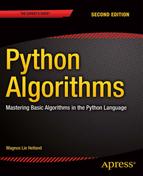
Reducing A to B is a bit like saying “You want to solve A? Oh, that’s easy, as long as you can solve B.” See Figure 4-1 for an illustration of how reductions work.
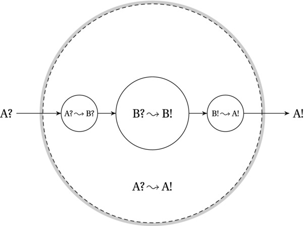
Figure 4-1. Using a reduction from A to B to solve A with an algorithm for B. The algorithm for B (the central, inner circle) can transform the input B? to the output B!, while the reduction consists of the two transformations (the smaller circles) going from A? to B? and from B! to A!, together forming the main algorithm, which transforms the input A? to the output A!
One, Two, Many
I’ve already used induction to solve some problems in Chapter 3, but let’s recap and work through a couple of examples. When describing induction in the abstract, we say that we have a proposition, or statement, P(n), and we want to show that it’s true for any natural number n. For example, let’s say we’re investigating the sum of the first n odd numbers; P(n) could then be the following statement:

This is eerily familiar—it’s almost the same as the handshake sum we worked with in the previous chapter. You could easily get this new result by tweaking the handshake formula, but let’s see how we’d prove it by induction instead. The idea in induction is to make our proof “sweep” over all the natural numbers, a bit like a row of dominoes falling. We start by establishing P(1), which is quite obvious in this case, and then we need to show that each domino, if it falls, will topple the next. In other words, we must show that if the statement P(n–1) is true, it follows that P(n) is also true.
If we can show this implication, that is, P(n–1) Þ P(n), the result will sweep across all values of n, starting with P(1), using P(1) Þ P(2) to establish P(2), then move on to P(3), P(4), and so forth. In other words, the crucial thing is to establish the implication that lets us move one step further. We call it the inductive step. In our example, this means that we’re assuming the following (P(n–1)):

We can take this for granted, and we just splice it into the original formula and see whether we can deduce P(n):
And there you go. The inductive step is established, and we now know that the formula holds for all natural numbers n.
The main thing that enables us to perform this inductive step is that we assume we’ve already established P(n–1). This means that we can start with what we know (or, rather, assume) about n–1 and build on that to show something about n. Let’s try a slightly less orderly example. Consider a rooted, binary tree where every internal node has two children (although it need not be balanced, so the leaves may all have different depths). If the tree has n leaves, how many internal nodes does it have?1
We no longer have a nice sequence of natural numbers, but the choice of induction variable (n) is pretty obvious. The solution (the number of internal nodes) is n–1, but now we need to show that this holds for all n. To avoid some boring technicalities, we start with n = 3, so we’re guaranteed a single internal node and two leaves (so clearly P(3) is true). Now, assume that for n–1 leaves, we have n–2 internal nodes. How do we take the crucial inductive step to n?
This is closer to how things work when building algorithms. Instead of just shuffling numbers and symbols, we’re thinking about structures, building them gradually. In this case, we’re adding a leaf to our tree. What happens? The problem is that we can’t just add leaves willy-nilly without violating the restrictions we’ve placed on the trees. Instead, we can work the step in reverse, from n leaves to n–1. In the tree with n leaves, remove any leaf along with its (internal) parent, and connect the two remaining pieces so that the now-disconnected node is inserted where the parent was. This is a legal tree with n–1 leaves and (by our induction assumption) n–2 internal nodes. The original tree had one more leaf and one more internal node, that is, n leaves and n–1 internals, which is exactly what we wanted to show.
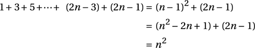
Now, consider the following classic puzzle. How do you cover a checkerboard that has one corner square missing, using L-shaped tiles, as illustrated in Figure 4-2? Is it even possible? Where would you start? You could try a brute-force solution, just starting with the first piece, placing it in every possible position (and with every possible orientation), and, for each of those, trying every possibility for the second, and so forth. That wouldn’t exactly be efficient. How can we reduce the problem? Where’s the reduction?2
Figure 4-2. An incomplete checkerboard, to be covered by L-shaped tiles. The tiles may be rotated, but they may not overlap
Placing a single tile and assuming that we can solve the rest or assuming that we’ve solved all but one and then placing the last one—that’s certainly a reduction. We’ve transformed the problem from one to another, but the catch is that we have no solution for the new problem either, so it doesn’t really help. To use induction (or recursion), the reduction must (generally) be between instances of the same problem of different sizes. For the moment, our problem is defined only for the specific board in Figure 4-2, but generalizing it to other sizes shouldn’t be too problematic. Given this generalization, do you see any useful reductions?
The question is how we can carve up the board into smaller ones of the same shape. It’s quadratic, so a natural starting point might be to split it into four smaller squares. The only thing standing between us and a complete solution at that point is that only one of the four board parts has the same shape as the original, with the missing corner. The other three are complete (quarter-size) checkerboards. That’s easily remedied, however. Just place a single tile so that it covers one corner from each of these three subboards, and, as if by magic, we now have four subproblems, each equivalent to (but smaller than) the full problem!
To clarify the induction here, let’s say you don’t actually place the tile quite yet. You just note which three corners to leave open. By the inductive hypothesis, you can cover the three subboards (with the base case being four-square boards), and once you’ve finished, there will be three squares left to cover, in an L-shape.3 The inductive step is then to place this piece, implicitly combining the four subsolutions. Now, because of induction, we haven’t only solved the problem for the eight-by-eight case; the solution holds for any board of this kind, as long as its sides are (equal) powers of two.
Note We haven’t really used induction over all board sizes or all side lengths here. We have implicitly assumed that the side lengths are 2k, for some positive integer k, and used induction over k. The result is perfectly valid, but it is important to note exactly what we’ve proven. The solution does not hold, for example, for odd-sided boards.
This design was really more of a proof than an actual algorithm. Turning it into an algorithm isn’t all that hard, though. You first need to consider all subproblems consisting of four squares, making sure to have their open corners properly aligned. Then you combine these into subproblems consisting of 16 squares, still making sure the open corners are placed so that they can be joined with L-pieces. Although you can certainly set this up as an iterative program with a loop, it turns out to be quite a bit easier with recursion, as you’ll see in the next section.
Mirror, Mirror
In his excellent web video show, Ze Frank once made the following remark: “‘You know there’s nothing to fear but fear itself.’ Yeah, that’s called recursion, and that would lead to infinite fear, so thank you.”4 Another common piece of advice is, “In order to understand recursion, one must first understand recursion.”
Indeed. Recursion can be hard to wrap your head around—although infinite recursion is a rather pathological case.5 In a way, recursion really makes sense only as a mirror image of induction (see Figure 4-3). In induction, we (conceptually) start with a base case and show how the inductive step can take us further, up to the full problem size, n. For weak induction,6 we assume (the inductive hypothesis) that our solution works for n–1, and from that, we deduce that it works for n. Recursion usually seems more like breaking things down. You start with a full problem, of size n. You delegate the subproblem of size n–1 to a recursive call, wait for the result, and extend the subsolution you get to a full solution. I’m sure you can see how this is really just a matter of perspective. In a way, induction shows us why recursion works, and recursion gives us an easy way of (directly) implementing our inductive ideas.
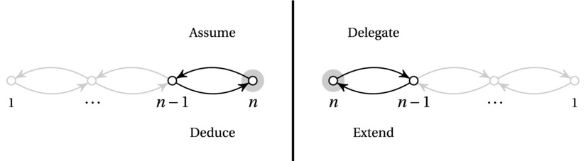
Figure 4-3. Induction (on the left) and recursion (on the right), as mirror images of each other
Take the checkerboard problem from the previous section, for example. The easiest way of formulating a solution to that (at least in my opinion) is recursive. You place an L-piece so that you get four equivalent subproblems, and then you solve them recursively. By induction, the solution will be correct.
IMPLEMENTING THE CHECKERBOARD COVERING
Although the checkerboard covering problem has a very easy recursive solution conceptually, implementing it can require a bit of thinking. The details of the implementation aren’t crucial to the main point of the example, so feel free to skip this sidebar, if you want. One way of implementing a solution is shown here:
def cover(board, lab=1, top=0, left=0, side=None):
if side is None: side = len(board)
# Side length of subboard:
s = side // 2
# Offsets for outer/inner squares of subboards:
offsets = (0, -1), (side-1, 0)
for dy_outer, dy_inner in offsets:
for dx_outer, dx_inner in offsets:
# If the outer corner is not set...
if not board[top+dy_outer][left+dx_outer]:
# ... label the inner corner:
board[top+s+dy_inner][left+s+dx_inner] = lab
# Next label:
lab += 1
if s > 1:
for dy in [0, s]:
for dx in [0, s]:
# Recursive calls, if s is at least 2:
lab = cover(board, lab, top+dy, left+dx, s)
# Return the next available label:
return lab
Although the recursive algorithm is simple, there is some bookkeeping to do. Each call needs to know which subboard it’s working on and the number (or label) of the current L-tile. The main work in the function is checking which of the four center squares to cover with the L-tile. We cover only the three that don’t correspond to a missing (outer) corner. Finally, there are four recursive calls, one for each of the four subproblems. (The next available label is returned, so it can be used in the next recursive call.) Here’s an example of how you might run the code:
>>> board = [[0]*8 for i in range(8)] # Eight by eight checkerboard
>>> board[7][7] = -1 # Missing corner
>>> cover(board)
22
>>> for row in board:
... print((" %2i"*8) % tuple(row))
3 3 4 4 8 8 9 9
3 2 2 4 8 7 7 9
5 2 6 6 10 10 7 11
5 5 6 1 1 10 11 11
13 13 14 1 18 18 19 19
13 12 14 14 18 17 17 19
15 12 12 16 20 17 21 21
15 15 16 16 20 20 21 -1
As you can see, all the numerical labels form L-shapes (except for -1, which represents the missing corner). The code can be a bit hard to understand, but imagine understanding it, not to mention designing it, without a basic knowledge of induction or recursion!
Induction and recursion go hand in hand in that it is often possible to directly implement an inductive idea recursively. However, there are several reasons why an iterative implementation may be superior. There is usually less overhead with using a loop than with recursion (so it can be faster), and in most languages (Python included), there is a limit to how deep the recursion can go (the maximum stack depth). Take the following example, which just traverses a sequence:
>>> def trav(seq, i=0):
...     if i==len(seq): return
...     trav(seq, i+1)
...
>>> trav(range(100))
>>>
It works, but try running it on range(1000). You’ll get a RuntimeError complaining that you’ve exceeded the maximum recursion depth.
Note Many so-called functional programming languages implement something called tail recursion optimization. Functions like the previous (where the only recursive call is the last statement of a function) are modified so that they don’t exhaust the stack. Typically, the recursive calls are rewritten to loops internally.
Luckily, any recursive function can be rewritten into an iterative one, and vice versa. In some cases, recursion is very natural, though, and you may need to fake it in your iterative program, using a stack of your own (as in nonrecursive depth-first search, explained in Chapter 5).
Let’s look at a couple of basic algorithms where the algorithmic idea can be easily understood by thinking recursively but where the implementation lends itself well to iteration.7 Consider the problem of sorting (a favorite in teaching computer science). As before, ask yourself, where’s the reduction? There are many ways of reducing this problem (in Chapter 6 we’ll be reducing it by half), but consider the case where we reduce the problem by one element. Either we can assume (inductively) that the first n–1 elements are already sorted and insert element n in the right place, or we can find the largest element, place it at position n, and then sort the remaining elements recursively. The former gives us insertion sort, while the latter gives selection sort.
Note These algorithms aren’t all that useful, but they’re commonly taught because they serve as excellent examples. Also, they’re classics, so any algorist should know how they work.
Take a look at the recursive insertion sort in Listing 4-1. It neatly encapsulates the algorithmic idea. To get the sequence sorted up to position i, first sort it recursively up to position i–1 (correct by the induction hypothesis) and then swap element seq[i] down until it reaches its correct position among the already sorted elements. The base case is when i = 0; a single element is trivially sorted. If you wanted, you could add a default case, where i is set to len(seq)-1. As explained, even though this implementation lets us encapsulate the induction hypothesis in a recursive call, it has practical limitations (for example, in the length of the sequence it’ll work on).
Listing 4-1. Recursive Insertion Sort
def ins_sort_rec(seq, i):
    if i==0: return                             # Base case -- do nothing
    ins_sort_rec(seq, i-1)                      # Sort 0..i-1
    j = i                                       # Start "walking" down
    while j > 0 and seq[j-1] > seq[j]:          # Look for OK spot
        seq[j-1], seq[j] = seq[j], seq[j-1]     # Keep moving seq[j] down
        j -= 1                                  # Decrement j
Listing 4-2 shows the iterative version more commonly known as insertion sort. Instead of recursing backward, it iterates forward, from the first element. If you think about it, that’s exactly what the recursive version does too. Although it seems to start at the end, the recursive calls go all the way back to the first element before the while loop is ever executed. After that recursive call returns, the while loop is executed on the second element, and so on, so the behaviors of the two versions are identical.
Listing 4-2. Insertion Sort
def ins_sort(seq):
    for i in range(1,len(seq)):                 # 0..i-1 sorted so far
        j = i                                   # Start "walking" down
        while j > 0 and seq[j-1] > seq[j]:      # Look for OK spot
            seq[j-1], seq[j] = seq[j], seq[j-1] # Keep moving seq[j] down
            j -= 1                              # Decrement j
Listings 4-3 and 4-4 contain a recursive and an iterative version of selection sort, respectively.
Listing 4-3. Recursive Selection Sort
def sel_sort_rec(seq, i):
    if i==0: return                             # Base case -- do nothing
    max_j = i                                   # Idx. of largest value so far
    for j in range(i):                          # Look for a larger value
        if seq[j] > seq[max_j]: max_j = j       # Found one? Update max_j
    seq[i], seq[max_j] = seq[max_j], seq[i]     # Switch largest into place
    sel_sort_rec(seq, i-1)                      # Sort 0..i-1
Listing 4-4. Selection Sort
def sel_sort(seq):
    for i in range(len(seq)-1,0,-1):            # n..i+1 sorted so far
        max_j = i                               # Idx. of largest value so far
        for j in range(i):                      # Look for a larger value
            if seq[j] > seq[max_j]: max_j = j   # Found one? Update max_j
        seq[i], seq[max_j] = seq[max_j], seq[i] # Switch largest into place
Once again, you can see that the two are quite similar. The recursive implementation explicitly represents the inductive hypothesis (as a recursive call), while the iterative version explicitly represents repeatedly performing the inductive step. Both work by finding the largest element (the for loop looking for max_j) and swapping that to the end of the sequence prefix under consideration. Note that you could just as well run all the four sorting algorithms in this section from the beginning, rather than from the end (sort all objects to the right in insertion sort or look for the smallest element in selection sort).
BUT WHERE IS THE REDUCTION?
Finding a useful reduction is often a crucial step in solving an algorithmic problem. If you don’t know where to b egin, ask yourself, where is the reduction?
However, it may not be entirely clear how the ideas in this section jibe with the picture of a reduction presented in Figure 4-1. As explained, a reduction transforms instances from problem A to instances of problem B and then transforms the output of B to valid output for A. But in induction and reduction, we’ve only reduced the problem size. Where is the reduction, really?
Oh, it’s there—it’s just that we’re reducing from A to A. There is some transformation going on, though. The reduction makes sure the instances we’re reducing to are smaller than the original (which is what makes the induction work), and when transforming the output, we increase the size again.
These are two major variations of reductions: reducing to a different problem and reducing to a shrunken version of the same. If you think of the subproblems as vertices and the reductions as edges, you get the subproblem graph discussed in Chapter 2, a concept I’ll revisit several times. (It’s especially important in Chapter 8.)
Designing with Induction (and Recursion)
In this section, I’ll walk you through the design of algorithmic solutions to three problems. The problem I’m building up to, topological sorting, is one that occurs quite a bit in practice and that you may very well need to implement yourself one day, if your software manages any kind of dependencies. The first two problems are perhaps less useful, but great fun, and they’re good illustrations of induction (and recursion).
Eight persons with very particular tastes have bought tickets to the movies. Some of them are happy with their seats, but most of them are not, and after standing in line in Chapter 3, they’re getting a bit grumpy. Let’s say each of them has a favorite seat, and you want to find a way to let them switch seats to make as many people as possible happy with the result (ignoring other audience members, who may eventually get a bit tired by the antics of our moviegoers). However, because they are all rather grumpy, all of them refuse to move to another seat if they can’t get their favorite.
This is a form of matching problem. You’ll encounter a few other of those in Chapter 10. We can model the problem (instance) as a graph, like the one in Figure 4-4. The edges point from where people are currently sitting to where they want to sit. (This graph is a bit unusual in that the nodes don’t have unique labels; each person, or seat, is represented twice.)
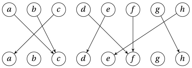
Figure 4-4. A mapping from the set {a ... h} to itself
Note This is an example of what’s called a bipartite graph, which means that the nodes can be partitioned into two sets, where all the edges are between the sets (and none of them inside either). In other words, you could color the nodes using only two colors so that no neighbors had the same color.
Before we try to design an algorithm, we need to formalize the problem. Truly understanding the problem is always a crucial first step in solving it. In this case, we want to let as many people as possible get the seat they’re “pointing to.” The others will need to remain seated. Another way of viewing this is that we’re looking for a subset of the people (or of the pointing fingers) that forms a one-to-one mapping, or permutation. This means that no one in the set points outside it, and each seat (in the set) is pointed to exactly once. That way, everyone in the permutation is free to permute—or switch seats—according to their wishes. We want to find a permutation that is as large as possible (to reduce the number of people that fall outside it and have their wishes denied).
Once again, our first step is to ask, where is the reduction? How can we reduce the problem to a smaller one? What subproblem can we delegate (recursively) or assume (inductively) to be solved already? Let’s go with simple (weak) induction and see whether we can shrink the problem from n to n–1. Here, n is the number of people (or seats), that is, n = 8 for Figure 4-4. The inductive assumption follows from our general approach. We simply assume that we can solve the problem (that is, find a maximum subset that forms a permutation) for n–1 people. The only thing that requires any creative problem solving is safely removing a single person so that the remaining subproblem is one that we can build on (that is, one that is part of a total solution).
If each person points to a different seat, the entire set forms a permutation, which must certainly be as big as it can be—no need to remove anyone because we’re already done. The base case is also trivial. For n = 1, there is nowhere to move. So, let’s say that n > 1 and that at least two persons are pointing to the same seat (the only way the permutation can be broken). Take a and b in Figure 4-4, for example. They’re both pointing to c, and we can safely say that one of them must be eliminated. However, which one we choose is crucial. Say, for example, we choose to remove a (both the person and the seat). We then notice that c is pointing to a, which means that c must also be eliminated. Finally, b points to c and must be eliminated as well—meaning that we could have simply eliminated b to begin with, keeping a and c (who just want to trade seats with each other).
When looking for inductive steps like this, it can often be a good idea to look for something that stands out. What, for example, about a seat that no one wants to sit in (that is, a node in the lower row in Figure 4-4 that has no in-edges)? In a valid solution (a permutation), at most one person (element) can be placed in (mapped to) any given seat (position). That means there’s no room for empty seats, because at least two people will then be trying to sit in the same seat. In other words, it is not only OK to remove an empty seat (and the corresponding person); it’s actually necessary. For example, in Figure 4-4, the nodes marked b cannot be part of any permutation, certainly not one of maximum size. Therefore, we can eliminate b, and what remains is a smaller instance (with n = 7) of the same problem , and, by the magic of induction, we’re done!
Or are we? We always need to make certain we’ve covered every eventuality. Can we be sure that there will always be an empty seat to eliminate, if needed? Indeed we can. Without empty seats, the n persons must collectively point to all the n seats, meaning that they all point to different seats, so we already have a permutation.
It’s time to translate the inductive/recursive algorithm idea into an actual implementation. An early decision is always how to represent the objects in the problem instances. In this case, we might think in terms of a graph or perhaps a function that maps between the objects. However, in essence, a mapping like this is just a position (0...n–1) associated with each element (also 0...n–1), and we can implement this using a simple list. For example, the example in Figure 4-4 (if a = 0, b = 1, ...) can be represented as follows:
>>> M = [2, 2, 0, 5, 3, 5, 7, 4]
>>> M[2] # c is mapped to a
0
Tip When possible, try to use a representation that is as specific to your problem as possible. More general representations can lead to more bookkeeping and complicated code; if you use a representation that implicitly embodies some of the constraints of the problem, both finding and implementing a solution can be much easier.
We can now implement the recursive algorithm idea directly if we want, with some brute-force code for finding the element to eliminate. It won’t be very efficient, but an inefficient implementation can sometimes be an instructive place to start. See Listing 4-5 for a relatively direct implementation.
Listing 4-5. A Naïve Implementation of the Recursive Algorithm Idea for Finding a Maximum Permutation
def naive_max_perm(M, A=None):
    if A is None:                               # The elt. set not supplied?
        A = set(range(len(M)))                  # A = {0, 1, ... , n-1}
    if len(A) == 1: return A                    # Base case -- single-elt. A
    B = set(M[i] for i in A)                    # The "pointed to" elements
    C = A - B                                   # "Not pointed to" elements
    if C:                                       # Any useless elements?
        A.remove(C.pop())                       # Remove one of them
        return naive_max_perm(M, A)             # Solve remaining problem
    return A                                    # All useful -- return all
The function naive_max_perm receives a set of remaining people (A) and creates a set of seats that are pointed to (B). If it finds an element in A that is not in B, it removes the element and solves the remaining problem recursively. Let’s use the implementation on our example, M.8
>>> naive_max_perm(M)
{0, 2, 5}
So, a, c, and f can take part in the permutation. The others will have to sit in nonfavorite seats.
The implementation isn’t too bad. The handy set type lets us manipulate sets with ready-made high-level operations, rather than having to implement them ourselves. There are some problems, though. For one thing, we might want an iterative solution. This is easily remedied—the recursion can quite simply be replaced by a loop (like we did for insertion sort and selection sort). A worse problem, though, is that the algorithm is quadratic! (Exercise 4-10 asks you to show this.)
The most wasteful operation is the repeated creation of the set B. If we could just keep track of which chairs are no longer pointed to, we could eliminate this operation entirely. One way of doing this would be to keep a count for each element. We could decrement the count for chair x when a person pointing to x is eliminated, and if x ever got a count of zero, both person and chair x would be out of the game.
Tip This idea of reference counting can be useful in general. It is, for example, a basic component in many systems for garbage collection (a form of memory management that automatically deallocates objects that are no longer useful). You’ll see this technique again in the discussion of topological sorting.
There may be more than one element to be eliminated at any one time, but we can just put any new ones we come across into a “to-do” list and deal with them later. If we needed to make sure the elements were eliminated in the order in which we discover that they’re no longer useful, we would need to use a first-in, first-out queue such as the deque class (discussed in Chapter 5).9 We don’t really care, so we could use a set, for example, but just appending to and popping from a list will probably give us quite a bit less overhead. But feel free to experiment, of course. You can find an implementation of the iterative, linear-time version of the algorithm in Listing 4-6.
Listing 4-6. Finding a Maximum Permutation
def max_perm(M):
    n = len(M)                                  # How many elements?
    A = set(range(n))                           # A = {0, 1, ... , n-1}
    count = [0]*n                               # C[i] == 0 for i in A
    for i in M:                                 # All that are "pointed to"
        count[i] += 1                           # Increment "point count"
    Q = [i for i in A if count[i] == 0]         # Useless elements
    while Q:                                    # While useless elts. left...
        i = Q.pop()                             # Get one
        A.remove(i)                             # Remove it
        j = M[i]                                # Who's it pointing to?
        count[j] -= 1                           # Not anymore...
        if count[j] == 0:                       # Is j useless now?
            Q.append(j)                         # Then deal w/it next
    return A                                    # Return useful elts.
Tip In recent versions of Python, the collections module contains the Counter class, which can count (hashable) objects for you. With it, the for loop in Listing 4-7 could have been replaced with the assignment count = Counter(M). This might have some extra overhead, but it would have the same asymptotic running time.
Listing 4-7. A Naïve Solution to the Celebrity Problem
def naive_celeb(G):
    n = len(G)
    for u in range(n):                          # For every candidate...
        for v in range(n):                      # For everyone else...
            if u == v: continue                 # Same person? Skip.
            if G[u][v]: break                   # Candidate knows other
            if not G[v][u]: break               # Other doesn't know candidate
        else:
            return u                            # No breaks? Celebrity!
    return None                                 # Couldn't find anyone
Some simple experiments (see Chapter 2 for tips) should convince you that even for rather small problem instances, max_perm is quite a bit faster than naive_max_perm. They’re both pretty fast, though, and if all you’re doing is solving a single, moderately sized instance, you might be just as satisfied with the more direct of the two. The inductive thinking would still have been useful in providing you with a solution that could actually find the answer. You could, of course, have tried every possibility, but that would have resulted in a totally useless algorithm. If, however, you had to solve some really large instances of this problem or even if you had to solve many moderate instances, the extra thinking involved in coming up with a linear-time algorithm would probably pay off.
COUNTING SORT & FAM
If the elements you’re working with in some problem are hashable or, even better, integers that you can use directly as indices (like in the permutation example), counting should be a tool you keep close at hand. One of the most well-known (and really, really pretty) examples of what counting can do is counting sort. As you’ll see in Chapter 6, there is a (loglinear) limit to how fast you can sort (in the worst case), if all you know about your values is whether they’re greater/less than each other.
In many cases, this is a reality you have to accept, for example, if you’re sorting objects with custom comparison methods. And loglinear is much better than the quadratic sorting algorithms we’ve seen so far. However, if you can count your elements, you can do better. You can sort in linear time! And what’s more, the counting sort algorithm is really simple. (And did I mention how pretty it is?)
from collections import defaultdict
def counting_sort(A, key=lambda x: x):
B, C = [], defaultdict(list) # Output and "counts"
for x in A:
C[key(x)].append(x) # "Count" key(x)
for k in range(min(C), max(C)+1): # For every key in the range
B.extend(C[k]) # Add values in sorted order
return B
By default, I’m just sorting objects based on their values. By supplying a key function, you can sort by anything you’d like. Note that the keys must be integers in a limited range. If this range is 0...k–1, the running time is then Θ(n + k). (Although the common implementation simply counts the elements and then figures out where to put them in B, Python makes it easy to just build value lists for each key and then concatenate them.) If several values have the same key, they’ll end up in the original order with respect to each other. Sorting algorithms with this property are called stable.
Counting-sort does need more space than an in-place algorithm like Quicksort, for example, so if your data set and value range is large, you might get a slowdown from a lack of memory. This can partly be handled by handling the value range more efficiently. We can do this by sorting numbers on individual digits (or strings on individual characters or bit vectors on fixed-size chunks). If you first sort on the least significant digit, because of stability, sorting on the second least significant digit won’t destroy the internal ordering from the first run. (This is a bit like sorting column by column in a spreadsheet.) This means that for d digits, you can sort n numbers in Θ(dn) time. This algorithm is called radix sort, and Exercise 4-11 asks you to implement it.
Another somewhat similar linear-time sorting algorithm is bucket sort. It assumes that your values are evenly (uniformly) distributed in an interval, for example, real numbers in the interval [0,1), and uses n buckets, or subintervals, that you can put your values into directly. In a way, you’re hashing each value into its proper slot, and the average (expected) size of each bucket is Θ(1). Because the buckets are in order, you can go through them and have your sorting in Θ(n) time, in the average case, for random data. (Exercise 4-12 asks you to implement bucket sort.)
The Celebrity Problem
In the celebrity problem, you’re looking for a celebrity in a crowd. It’s a bit far-fetched, though it could perhaps be used in analyses of social networks such as Facebook and Twitter. The idea is as follows: The celebrity knows no one, but everyone knows the celebrity.10 A more down-to-earth version of the same problem would be examining a set of dependencies and trying to find a place to start. For example, you might have threads in a multithreaded application waiting for each other, with even some cyclical dependencies (so-called deadlocks), and you’re looking for one thread that isn’t waiting for any of the others but that all of the others are dependent on. (A much more realistic way of handling dependencies—topological sorting—is dealt with in the next section.)
No matter how we dress the problem up, its core can be represented in terms of graphs. We’re looking for one node with incoming edges from all other nodes, but with no outgoing edges. Having gotten a handle on the structures we’re dealing with, we can implement a brute-force solution, just to see whether it helps us understand anything (see Listing 4-7).
The naive_celeb function tackles the problem head on. Go through all the people, checking whether each person is a celebrity. This check goes through all the others, making sure they all know the candidate person and that the candidate person does not know any of them. This version is clearly quadratic, but it’s possible to get the running time down to linear.
The key, as before, lies in finding a reduction—reducing the problem from n persons to n–1 as cheaply as possible. The naive_celeb implementation does, in fact, reduce the problem step by step. In iteration k of the outer loop, we know that none of 0...k–1 can be the celebrity, so we need to solve the problem only for the remainder, which is exactly what the remaining iterations do. This reduction is clearly correct, as is the algorithm. What’s new in this situation is that we have to try to improve the efficiency of the reduction. To get a linear algorithm, we need to perform the reduction in constant time. If we can do that, the problem is as good as solved. As you can see, this inductive way of thinking can really help pinpoint where we need to employ our creative problem-solving skills.
Once we’ve zeroed in on what we need to do, the problem isn’t all that hard. To reduce the problem from n to n–1, we must find a noncelebrity, someone who either knows someone or is unknown by someone else. And if we check G[u][v] for any nodes u and v, we can eliminate either u or v! If G[u][v] is true, we eliminate u; otherwise, we eliminate v. If we’re guaranteed that there is a celebrity, this is all we need. Otherwise, we can still eliminate all but one candidate, but we need to finish by checking whether they are, in fact, a celebrity, like we did in naive_celeb. You can find an implementation of the algorithm based on this reduction in Listing 4-8. (You could implement the algorithm idea even more directly using sets; do you see how?)
Listing 4-8. A Solution to the Celebrity Problem
def celeb(G):
    n = len(G)
    u, v = 0, 1                                 # The first two
    for c in range(2,n+1):                      # Others to check
        if G[u][v]: u = c                       # u knows v? Replace u
        else:       v = c                       # Otherwise, replace v
    if u == n:      c = v                       # u was replaced last; use v
    else:           c = u                       # Otherwise, u is a candidate
    for v in range(n):                          # For everyone else...
        if c == v: continue                     # Same person? Skip.
        if G[c][v]: break                       # Candidate knows other
        if not G[v][c]: break                   # Other doesn't know candidate
    else:
        return c                                # No breaks? Celebrity!
    return None                                 # Couldn't find anyone
To try these celebrity-finding functions, you can just whip up a random graph.11 Let’s switch each edge on or off with equal probability:
>>> from random import randrange
>>> n = 100
>>> G = [[randrange(2) for i in range(n)] for i in range(n)]
Now make sure there is a celebrity in there and run the two functions:
>>> c = randrange(n)
>>> for i in range(n):
...     G[i][c] = True
...     G[c][i] = False
...
>>> naive_celeb(G)
57
>>> celeb(G)
57
Note that though one is quadratic and one is linear, the time to build the graph (whether random or from some other source) is quadratic here. That could be avoided (for a sparse graph, where the average number of edges is less than Θ(n)), with some other graph representation; see Chapter 2 for suggestions.
Topological Sorting
In almost any project, the tasks to be undertaken will have dependencies that partially restrict their ordering. For example, unless you have a very avant-garde fashion sense, you need to put on your socks before your boots, but whether you put on your hat before your shorts is of less importance. Such dependencies are (as mentioned in Chapter 2) easily represented as a directed acyclic graph (DAG), and finding an ordering that respect the dependencies (so that all the edges point forward in the ordering) is called topological sorting.
Figure 4-5 illustrates the concept. In this case, there is a unique valid ordering, but consider what would happen if you removed the edge ab, for example—then a could be placed anywhere in the order, as long as it was before f.
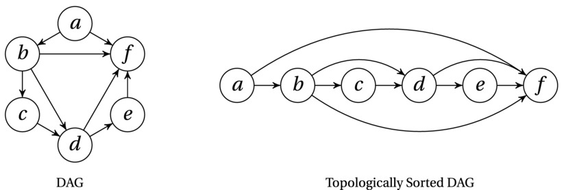
Figure 4-5. A directed acyclic graph (DAG) and its nodes in topologically sorted order
The problem of topological sorting occurs in many circumstances in any moderately complex computer system. Things need to be done, and they depend on other things ... where to start? A rather obvious example is installing software. Most modern operating systems have at least one system for automatically installing software components (such as applications or libraries), and these systems can automatically detect when some dependency is missing and then download and install it. For this to work, the components must be installed in a topologically sorted order.12
There are also algorithms (such as the one for finding shortest paths in DAGs and, in a sense, most algorithms based on dynamic programming) that are based on a DAG being sorted topologically as an initial step. However, while standard sorting algorithms are easy to encapsulate in standard libraries and the like, abstracting away graph algorithms so they work with any kind of dependency structure is a bit harder ... so the odds aren’t too bad that you’ll need to implement it at some point.
Tip If you’re using a Unix system of some sort, you can play around with topological sorting of graphs described in plain-text files, using the tsort command.
We already have a good representation of the structures in our problem (a DAG). The next step is to look for some useful reduction. As before, our first intuition should probably be to remove a node and solve the problem (or assume that it is already solved) for the remaining n–1. This reasonably obvious reduction can be implemented in a manner similar to insertion sort, as shown in Listing 4-9. (I’m assuming adjacency sets or adjacency dicts or the like here; see Chapter 2 for details.)
Listing 4-9. A Naïve Algorithm for Topological Sorting
def naive_topsort(G, S=None):
    if S is None: S = set(G)                    # Default: All nodes
    if len(S) == 1: return list(S)              # Base case, single node
    v = S.pop()                                 # Reduction: Remove a node
    seq = naive_topsort(G, S)                   # Recursion (assumption), n-1
    min_i = 0
    for i, u in enumerate(seq):
        if v in G[u]: min_i = i+1               # After all dependencies
    seq.insert(min_i, v)
    return seq
Although I hope it’s clear (by induction) that naive_topsort is correct, it is also clearly quadratic (by recurrence 2 from Table 3-1). The problem is that it chooses an arbitrary node at each step, which means that it has to look where the node fits after the recursive call (which gives the linear work). We can turn this around and work more like selection sort. Find the right node to remove before the recursive call. This new idea, however, leaves us with two questions. First, which node should we remove? And second, how can we find it efficiently?13
We’re working with a sequence (or at least we’re working toward a sequence), which should perhaps give us an idea. We can do something similar to what we do in selection sort and pick out the element that should be placed first (or last ... it doesn’t really matter; see Exercise 4-19). Here, we can’t just place it first—we need to really remove it from the graph, so the rest is still a DAG (an equivalent but smaller problem). Luckily, we can do this without changing the graph representation directly, as you’ll see in a minute.
How would you find a node that can be put first? There could be more than one valid choice, but it doesn’t matter which one you take. I hope this reminds you of the maximum permutation problem. Once again, we want to find the nodes that have no in-edges. A node without in-edges can safely be placed first because it doesn’t depend on any others. If we (conceptually) remove all its out-edges, the remaining graph, with n–1 nodes, will also be a DAG that can be sorted in the same way.
Tip If a problem reminds you of a problem or an algorithm you already know, that’s probably a good sign. In fact, building a mental archive of problems and algorithms is one of the things that can make you a skilled algorist. If you’re faced with a problem and you have no immediate associations, you could systematically consider any relevant (or semirelevant) techniques you know and look for reduction potential.
Just like in the maximum permutation problem, we can find the nodes without in-edges by counting. By maintaining our counts from one step to the next, we need not start fresh each time, which reduces the linear step cost to a constant one (yielding a linear running time in total, as in recurrence 1 in Table 3-1). Listing 4-10 shows an iterative implementation of this counting-based topological sorting. (Can you see how the iterative structure still embodies the recursive idea?) The only assumption about the graph representation is that we can iterate over the nodes and their neighbors.
Listing 4-10. Topological Sorted of a Directed, Acyclic Graph
def topsort(G):
    count = dict((u, 0) for u in G)             # The in-degree for each node
    for u in G:
        for v in G[u]:
            count[v] += 1                       # Count every in-edge
    Q = [u for u in G if count[u] == 0]         # Valid initial nodes
    S = []                                      # The result
    while Q:                                    # While we have start nodes...
        u = Q.pop()                             # Pick one
        S.append(u)                             # Use it as first of the rest
        for v in G[u]:
            count[v] -= 1                       # "Uncount" its out-edges
            if count[v] == 0:                   # New valid start nodes?
                Q.append(v)                     # Deal with them next
    return S
BLACK BOX: TOPOLOGICAL SORTING AND PYTHON’S MRO
The kind of structural ordering we’ve been working with in this section is actually an integral part of Python object-oriented inheritance semantics. For single inheritance (each class is derived from a single superclass), picking the right attribute or method to use is easy. Simply walk upward in the “chain of inheritance,” first checking the instance, then the class, then the superclass, and so forth. The first class that has what we’re looking for is used.
However, if you can have more than one superclass, things get a bit tricky. Consider the following example:
>>> class X: pass
>>> class Y: pass
>>> class A(X,Y): pass
>>> class B(Y,X): pass
If you were to derive a new class C from A and B, you’d be in trouble. You wouldn’t know whether to look for methods in X or Y.
In general, the inheritance relationship forms a DAG (you can’t inherit in a cycle), and in order to figure out where to look for methods, most languages create a linearization of the classes, which is simply a topological sorting of the DAG. Recent versions of Python use a method resolution order (or MRO) called C3 (see the references for more information), which in addition to linearizing the classes in a way that makes as much sense as possible also prohibits problematic cases such as the one in the earlier example.
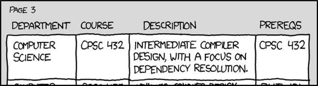
Dependencies. The prereqs for CPSC 357, the class on package management, are CPSC 432, CPSC 357, and glibc2.5 or later (http://xkcd.com/754)
Stronger Assumptions
The default induction hypothesis when designing algorithm is “We can solve smaller instances with this,” but sometimes that isn’t enough to actually perform the induction step or to perform it efficiently. Choosing the order of the subproblems can be important (such as in topological sorting), but sometimes we must actually make a stronger assumption to piggyback some extra information on our induction. Although a stronger assumption might seem to make the proof harder,14 it actually just gives us more to work with when deducing the step from n–1 (or n/2, or some other size) to n.
Consider the idea of balance factors. These are used in some types of balanced trees (discussed in Chapter 6) and are a measure of how balanced (or unbalanced) a tree or subtree is. For simplicity, we assume that each internal node has two children. (In an actual implementation, some of the leaves might simply be None or the like.) A balance factor is defined for each internal node and is set to the difference between the heights of the left and right subtrees, where height is the greatest distance from the node (downward) to a leaf. For example, the left child of the root in Figure 4-6 has a balance factor of –2 because its left subtree is a leaf (with a height of 0), while its right child has a height of 2.
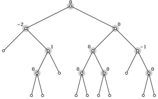
Figure 4-6. Balance factors for a binary tree. The balance factors are defined only for internal nodes (highlighted) but could trivially be set to zero for leaves
Calculating balance factors isn’t a very challenging algorithm design problem, but it does illustrate a point. Consider the obvious (divide-and-conquer) reduction. To find the balance factor for the root, solve the problem recursively for each subtree and then extend/combine the partial solutions to a complete solution. Easy peasy. Except ... it won’t work. The inductive assumption that we can solve smaller subproblems won’t help us here because the solution (that is, the balance factor) for our subproblems doesn’t contain enough information to make the inductive step! The balance factor isn’t defined in terms of its children’s balance factors—it’s defined in terms of their heights. We can easily solve this by just strengthening our assumption. We assume that we can find the balance factors and the heights of any tree with k < n nodes. We can now use the heights in the inductive step, finding both the balance factor (left height minus right height) and the height (max of left and right height, plus one) for size n in our inductive step. Problem solved! Exercise 4-20 asks you to work out the details here.
Note Recursive algorithms over trees are intimately linked with depth-first search, discussed in Chapter 5.
Thinking formally about strengthening the inductive hypothesis can sometimes be a bit confusing. Instead, you can just think about what extra information you need to “piggyback” on your inductive step in order to build a larger solution. For example, when working with topological sorting earlier, it was clear that piggybacking (and maintaining) the in-degrees while we were stepping through the partial solutions made it possible to perform the inductive step more efficiently.
For more examples of strengthening induction hypotheses, see the closest point problem in Chapter 6 and the interval containment problem in Exercise 4-21.
REVERSE INDUCTION AND POWERS OF TWO
Sometimes it can be useful to restrict the problem sizes we’re working with, such as dealing only with powers of two. This often occurs for divide-and-conquer algorithms, for example (see Chapters 3 and 6 for recurrences and examples, respectively). In many cases, whatever algorithms or complexities we find will still work for any value of n, but sometimes, as for the checkerboard covering problem described earlier in this chapter, this just isn’t the case. To be certain, we might need to prove that any value of n is safe. For recurrences, the induction method in Chapter 3 can be used. For showing correctness, you can use reverse induction. Assume that the algorithm is correct for n and show that this implies correctness for n – 1.This can often be done by simply introducing a “dummy” element that doesn’t affect the solution but that increases the size to n. If you know the algorithm is correct for an infinite set of sizes (such as all powers of two), reverse induction will let you show that it’s true for all sizes.
Invariants and Correctness
The main focus of this chapter is on designing algorithms, where correctness follows from the design process. Perhaps a more common perspective on induction in computer science is correctness proofs. It’s basically the same thing that I’ve been discussing in this chapter but with a slightly different angle of approach. You’re presented with a finished algorithm, and you need to show that it works. For a recursive algorithm, the ideas I’ve already shown you can be used rather directly. For a loop, you can also think recursively, but there is a concept that applies more directly to induction proofs for iteration: loop invariants. A loop invariant is something that is true after each iteration of a loop, given some preconditions; it’s called an invariant because it doesn’t vary—it’s true from beginning to end.
Usually, the final solution is the special case that the invariant attains after the final iteration, so if the invariant always holds (given the preconditions of the algorithm) and you can show that the loop terminates, you’ve shown that the algorithm is correct. Let’s try this approach with insertion sort (Listing 4-2). The invariant for the loop is that the elements 0...i are sorted (as hinted at by the first comment in the code). If we want to use this invariant to prove correctness, we need to do the following:
- Use induction to show that it is, in fact, true after each iteration.
- Show that we’ll get the correct answer if the algorithm terminates.
- Show that the algorithm terminates.
The induction in step 1 involves showing a base case (that is, before the first iteration) and an inductive step (that a single run of the loop preserves the invariant). The second step involves using the invariant at the point of termination. The third step is usually easy to prove (perhaps by showing that you eventually “run out” of something).15
Steps 2 and 3 should be obvious for insertion sort. The for loop will terminate after n iterations, with i = n–1. The invariant then says that elements 0...n–1 are sorted, which means that the problem is solved. The base case (i = 0) is trivial, so all that remains is the inductive step—to show that the loop preserves the invariant, which it does, by inserting the next element in the correct spot among the sorted values (without disrupting the sorting).
Relaxation and Gradual Improvement
The term relaxation is taken from mathematics, where it has several meanings. The term has been picked up by algorists and is used to describe the crucial step in several algorithms, particularly shortest-path algorithms based on dynamic programming (discussed in Chapters 8 and 9), where we gradually improve our approximations to the optimum. The idea of incrementally improving a solution in this way is also central to algorithms finding maximum flow (Chapter 10). I won’t go into how these algorithms work just yet, but let’s look at a simple example of something that might be called relaxation.
You are in an airport, and you can reach several other airports by plane. From each of those airports, you can take the train to several towns and cities. Let’s say that you have a dict or list of flight times, A, so that A[u] is the time it will take you to get to airport u. Similarly, B[u][v] will give you the time it takes to get from airport u to town v by train. (B can be a list of lists or a dict of dicts, for example; see Chapter 2.) Consider the following randomized way of estimating the time it will take you to get to each town, C[v]:
>>> for v in range(n):
...     C[v] = float('inf')
>>> for i in range(N):
...     u, v = randrange(n), randrange(n)
...     C[v] = min(C[v], A[u] + B[u][v]) # Relax
The idea here is to repeatedly see whether we can improve our estimate for C[v] by choosing another route. First go to u by plane, and then you take the train to v. If that gives us a better total time, we update C. As long as N is really large, we will eventually get the right answer for every town.
For relaxation-based algorithms that actually guarantee correct solutions, we need to do better than this. For the airplane + train problem, this is fairly easy (see Exercise 4-22). For more complex problems, you may need rather subtle approaches. For example, you can show that the value of your solution increases by an integer in every iteration; if the algorithm terminates only when you hit the optimal (integer) value, it must be correct. (This is similar to the case for maximum flow algorithms.) Or perhaps you need to show how correct estimates spread across elements of the problem instance, such as nodes in a graph. If this seems a bit general at the moment, don’t worry—I’ll get plenty specific when we encounter algorithms that use the technique.
Tip Designing algorithms with relaxation can be like a game. Each relaxation is one “move,” and you try to get the optimal solution with as few moves as possible. You can always get there by just relaxing all over the place, but the key lies in performing your moves in the right order. This idea will be explored further when we deal with shortest paths in DAGs (Chapter 8), Bellman-Ford, and Dijkstra’s algorithm (Chapter 9).
Reduction + Contraposition = Hardness Proof
This section is really just a bit of foreshadowing of what you’ll encounter in Chapter 11. You see, although reductions are used to solve problems, the only context in which most textbooks discuss them is problem complexity, where they’re used to show that you (probably) can’t solve a given problem. The idea is really quite simple, yet I’ve seen it trip up many (perhaps even most) of my students.
The hardness proofs are based on the fact that we only allow easy (that is, fast) reductions.16 Let’s say you’re able to reduce problem A to B (so a solution to B gives you one for A as well; take a look at Figure 4-1 if you need to refresh your memory on how this works). We then know that if B is easy, A must be easy as well. That follows directly from the fact that we can use B, along with an easy reduction, to solve A.
For example, let A be finding the longest path between two nodes in a DAG, and let B be finding the shortest path between two nodes in a DAG. You can then reduce A to B by simply viewing all edges as negative. Now, if you learn of some efficient algorithm to find shortest paths in DAGs that permits negative edge weights (which you will, in Chapter 8), you automatically also have an efficient algorithm for finding for longest paths with positive edge weights.17 The reason for this is that, with asymptotic notation (which is implicitly used here), you could say that “fast + fast = fast.” In other words, fast reduction + fast solution to B = fast solution to A.
Now let’s apply our friend contraposition. We’ve established “If B is easy, then A is easy.” The contrapositive is “If A is hard, then B is hard.”18 This should still be quite easy to understand, intuitively. If we know that A is hard, no matter how we approach it, we know B can’t be easy—because if it were easy, it would supply us with an easy solution to A, and A wouldn’t be hard after all (a contradiction).
I hope the section has made sense so far. Now there’s just one last step to the reasoning. If I come across a new, unknown problem X, and I already know that the problem Y is hard, how can I use a reduction to show that X is hard?
There are basically two alternatives, so the odds should be about 50-50. Oddly enough, it seems that more than half the people I ask get this wrong before they think about it a bit. The answer is, reduce Y to X. (Did you get it right?) If you know Y is hard and you reduce it to X, then X must be hard, because otherwise it could be used to solve Y easily—a contradiction.
Reducing in the other direction doesn’t really get you anywhere. For example, fixing a smashed computer is hard, but if you want to know whether fixing your (unsmashed) computer is easy or hard, smashing it isn’t going to prove anything.
So, to sum up the reasoning here:
- If you can (easily) reduce A to B, then B is at least as hard as A.
- If you want to show that X is hard and you know that Y is hard, reduce Y to X.
One of the reasons this is so confusing for many people is that we normally think of reductions as transforming a problem to something easier. Even the name “reduction” connotes this. However, if we’re solving A by reducing it to B, it only seems like B is easier, because it’s something we already know how to solve. After the reduction, A is just as easy—because we can solve it through B (with the addition of an easy, fast reduction). In other words, as long as your reduction isn’t doing any heavy lifting, you can never reduce to something easier, because the act of reduction automatically evens things out. Reduce A to B, and B is automatically at least as hard as A.
Let’s leave it at that for now. I’ll get into the details in Chapter 11.
Problem Solving Advice
Here is some advice for solving algorithmic problems and designing algorithms, summing up some of the main ideas of this chapter:
- Make sure you really understand the problem. What is the input? The output? What’s the precise relationship between the two? Try to represent the problem instances as familiar structures, such as sequences or graphs. A direct, brute-force solution can sometimes help clarify exactly what the problem is.
- Look for a reduction. Can you transform the input so it works as input for another problem that you can solve? Can you transform the resulting output so that you can use it? Can you reduce an instance of size n to an instance of size k < n and extend the recursive solution (inductive hypothesis) back to n?
Together, these two form a powerful approach to algorithm design. I’m going to add a third item here, as well. It’s not so much a third step as something to keep in mind while working through the first two:
- Are there extra assumptions you can exploit? Integers in a fixed value range can be sorted more efficiently than arbitrary values. Finding the shortest path in a DAG is easier than in an arbitrary graph, and using only non-negative edge weights is often easier than arbitrary edge weights.
At the moment, you should be able to start using the first two pieces of advice in constructing your algorithms. The first (understanding and representing the problem) may seem obvious, but a deep understanding of the structure of the problem can make it much easier to find a solution. Consider special cases or simplifications to see whether they give you ideas. Wishful thinking can be useful here, dropping parts of the problem specification, so you can think of one or a few aspects at a time. (“What if we ignored the edge weights? What if all the numbers were 0 or 1? What if all the strings were of equal length? What if every node had exactly k neighbors?”)
The second item (looking for a reduction) has been discussed a lot in this chapter, especially reducing to (or decomposing into) subproblems. This is crucial when designing your own spanking new algorithms, but ordinarily, it is much more likely that you’ll find an algorithm that almost fits. Look for patterns in or aspects of the problem that you recognize, and scan your mental archives for algorithms that might be relevant. Instead of constructing an algorithm that will solve the problem, can you construct an algorithm that will transform the instances so an existing algorithm can solve them? Working systematically with the problems and algorithms you know can be more productive than waiting for inspiration.
The third item is more of a general observation. Algorithms that are tailored to a specific problem are usually more efficient than more general algorithms. Even if you know a general solution, perhaps you can tweak it to use the extra constraints of this particular problem? If you’ve constructed a brute-force solution in an effort to understand the problem, perhaps you can develop that into a more efficient solution by using these quirks of the problem? Think of modifying insertion sort so it becomes bucket sort,19 for example, because you know something about the distribution of the values.
Summary
This chapter is about designing algorithms by somehow reducing a problem to something you know how to solve. If you reduce to a different problem entirely, you can perhaps solve it with an existing algorithm. If you reduce it to one or more subproblems (smaller instances of the same problem), you can solve it inductively, and the inductive design gives you a new algorithm. Most examples in this chapter have been based on weak induction or extending solutions to subproblems of size n–1. In later chapters, especially Chapter 6, you will see more use of strong induction, where the subproblems can be of any size k < n.
This sort of size reduction and induction is closely related to recursion. Induction is what you use to show that recursion is correct, and recursion is a very direct way of implementing most inductive algorithm ideas. However, rewriting the algorithm to be iterative can avoid the overhead and limitations of recursive functions in most nonfunctional programming languages. If an algorithm is iterative to begin with, you can still think of it recursively, by viewing the subproblem solved so far as if it were calculated by a recursive call. Another approach would be to define a loop invariant, which is true after every iteration and which you prove using induction. If you show that the algorithm terminates, you can use the invariant to show correctness.
Of the examples in this chapter, the most important one is probably topological sorting: ordering the nodes of a DAG so that all edges point forward (that is, so that all dependencies are respected). This is important for finding a valid order of performing tasks that depend on each other, for example, or for ordering subproblems in more complex algorithms. The algorithm presented here repeatedly removes nodes without in-edges, appending them to the ordering and maintaining in-degrees for all nodes to keep the solution efficient. Chapter 5 describes another algorithm for this problem.
In some algorithms, the inductive idea isn’t linked only to subproblem sizes. They are based on gradual improvement of some estimate, using an approach called relaxation. This is used in many algorithms for finding shortest paths in weighted graphs, for example. To prove that these are correct, you may need to uncover patterns in how the estimates improve or how correct estimates spread across elements of your problem instances.
While reductions have been used in this chapter to show that a problem is easy, that is, to find a solution for it, you can also use reductions to show that one problem is at least as hard as another. If you reduce problem A to problem B, and the reduction itself is easy, then B must be at least as hard as A (or we get a contradiction). This idea is explored in more detail in Chapter 11.
If You’re Curious ...
As I said in the introduction, this chapter is to a large extent inspired by Udi Manber’s paper “Using induction to design algorithms.” Information on both that paper and his later book on the same subject can be found in the “References” section. I highly recommend that you at least take a look at the paper, which you can probably find online. You will also encounter several examples and applications of these principles throughout the rest of the book.
If you really want to understand how recursion can be used for virtually anything, you might want to play around with a functional language, such as Haskell (see http://haskell.org) or Clojure (see http://clojure.org). Just going through some basic tutorials on functional programming could deepen your understanding of recursion, and, thereby, induction, greatly, especially if you’re a bit new to this way of thinking. You could even check out the books by Rabhi and Lapalme on algorithms in Haskell and by Okasaki on data structures in functional languages in general.
Although I’ve focused exclusively on the inductive properties of recursion here, there are other ways of showing how recursion works. For example, there exists a so-called fixpoint theory of recursion that can be used to determine what a recursive function really does. It’s rather heavy stuff, and I wouldn’t recommend it as a place to start, but if you want to know more about it, you could check out the book by Zohar Manna or (for a slightly easier but also less thorough description) the one by Michael Soltys.
If you’d like more problem-solving advice, Pólya’s How to Solve It is a classic, which keeps being reprinted. Worth a look. You might also want to get The Algorithm Design Manual by Steven Skiena. It’s a reasonably comprehensive reference of basic algorithms, along with a discussion of design principles. He even has a quite useful checklist for solving algorithmic problems.
Exercises
4-1. A graph that you can draw in the plane without any edges crossing each other is called planar. Such a drawing will have a number of regions, areas bounded by the edges of the graph, as well as the (infinitely large) area around the graph. If the graph has V, E, and F nodes, edges, and regions, respectively, Euler’s formula for connected planar graphs says that V – E + F = 2. Prove that this is correct using induction.
4-2. Consider a plate of chocolate, consisting of n squares in a rectangular arrangement. You want to break it into individual squares, and the only operation you’ll use is breaking one of the current rectangles (there will be more, once you start breaking) into two pieces. What is the most efficient way of doing this?
4-3. Let’s say you’re going to invite some people to a party. You’re considering n friends, but you know that they will have a good time only if each of them knows at least k others at the party. (Assume that if A knows B, then B automatically knows A.) Solve your problem by designing an algorithm for finding the largest possible subset of your friends where everyone knows at least k of the others, if such a subset exists.
Bonus question: If your friends know d others in the group on average and at least one person knows at least one other, show that you can always find a (nonempty) solution for k ≤ d/2.
4-4. A node is called central if the greatest (unweighted) distance from that node to any other in the same graph is minimum. That is, if you sort the nodes by their greatest distance to any other node, the central nodes will be at the beginning. Explain why an unrooted tree has either one or two central nodes, and describe an algorithm for finding them.
4-5. Remember the knights in Chapter 3? After their first tournament, which was a round-robin tournament, where each knight jousted one of the other, the staff want to create a ranking. They realize it might not be possible to create a unique ranking or even a proper topological sorting (because there may be cycles of knights defeating each other), but they have decided on the following solution: order the knights in a sequence K1, K2, ... , Kn, where K1 defeated K2, K2 defeated K3, and so forth (Ki–1 defeated Ki, for i=2...n). Prove that it is always possible to construct such a sequence by designing an algorithm that builds it.
4-6. George Pólya (the author of How to Solve It; see the “References” section) came up with the following entertaining (and intentionally fallacious) “proof” that all horses have the same color. If you have only a single horse, then there’s clearly only one color (the base case). Now we want to prove that n horses have the same color, under the inductive hypothesis that all sets of n–1 horses do. Consider the sets {1, 2, ... , n–1} and {2, 3, ... , n}. These are both of size n–1, so in each set, there is only one color. However, because the sets overlap, the same must be true for {1, 2, ... n}. Where’s the error in this argument?
4-7. In the example early in the section “One, Two, Many,” where we wanted to show how many internal nodes a binary tree with n leaves had, instead of “building up” from n–1 to n, we started with n nodes and deleted one leaf and one internal node. Why was that OK?
4-8. Use the standard rules from Chapter 2 and the recurrences from Chapter 3 and show that the running times of the four sorting algorithms in Listings 4-1 through 4-4 are all quadratic.
4-9. In finding a maximum permutation recursively (such as in Listing 4-5), how can we be sure that the permutation we end up with contains at least one person? Shouldn’t it be possible, in theory, to remove everyone?
4-10. Show that the naïve algorithm for finding the maximum permutation (Listing 4-5) is quadratic.
4-11. Implement radix sort.
4-12. Implement bucket sort.
4-13. For numbers (or strings or sequences) with a fixed number of digits (or characters or elements), d, radix sort has a running time of Θ(dn). Let’s say you are sorting number whose digit counts vary greatly. A standard radix sort would require you to set d to the maximum of these, padding the rest with initial zeros. If, for example, a single number had a lot more digits than all the others, this wouldn’t be very efficient. How could you modify the algorithm to have a running time of Θ(∑di), where di is the digit count of the ith number?
4-14. How could you sort n numbers in the value range 1...n2 in Θ(n) time?
4-15. When finding in-degrees in the maximum permutation problem, why could the count array simply be set to [M.count(i) for i in range(n)]?
4-16. The section “Designing with Induction (and Recursion)” describes solutions to three problems. Compare the naïve and final versions of the algorithms experimentally.
4-17. Explain why naive_topsort is correct; why is it correct to insert the last node directly after its dependencies?
4-18. Write a function for generating random DAGs. Write an automatic test that checks that topsort gives a valid orderings, using your DAG generator.
4-19. Redesign topsort so it selects the last node in each iteration, rather than the first.
4-20. Implement the algorithm for finding balance factors in a binary tree.
4-21. An interval can be represented, for example, as a pair of numbers, such as (3.2, 4.9). Let’s say you have a list of such intervals (where no intervals are identical), and you want know which intervals that fall inside other intervals. An interval (u,v) falls inside (x,y) when x ≤ u and v ≤ y. How would you do this efficiently?
4-22. How would you improve the relaxation-based algorithm for the airplane + train problem in the section “Relaxation and Gradual Improvement” so that you are guaranteed an answer in polynomial time?
4-23. Consider three problems, foo, bar, and baz. You know that bar is hard and that baz is easy. How would you go about showing that foo was hard? How would you show that it was easy?
References
Manber, U. (1988). Using induction to design algorithms. Communications of the ACM, 31(11):1300–1313.
Manber, U. (1989). Introduction to Algorithms: A Creative Approach. Addison-Wesley.
Manna, Z. (1974). Mathematical Theory of Computation. McGraw-Hill Book Company.
Okasaki, C. (1999). Purely Functional Data Structures. Cambridge University Press.
Pólya, G. (2009). How To Solve It: A New Aspect of Mathematical Method. Ishi Press.
Rabhi, F. A. and Lapalme, G. (1999). Algorithms: A Functional Approach. Addison-Wesley.
Simionato, M. (2006). The Python 2.3 method resolution order. http://python.org/download/releases/2.3/mro.
Skiena, S. S. (2008). The Algorithm Design Manual, second edition. Springer.
Soltys, M. (2010). An Introduction to the Analysis of Algorithms. World Scientific.
__________________
1This is actually Exercise 2-10, but you can still have a go at that, if you want. Try to solve it without using induction.
2Actually, the solution idea presented in the following will work for a checkerboard where an arbitrary square is missing. I recommend you verify that for yourself.
3An important part of this inductive hypothesis is that we can solve the problem no matter which corner is missing.
4the show with zefrank, February 22, 2007.
5Ever tried to search for recursion with Google? You might want to try it. And pay attention to the search suggestion.
6As mentioned in Chapter 3, in weak induction the induction hypothesis applies to n–1, while in strong induction it applies to all positive integers k < n.
7These algorithms aren’t all that useful, but they’re commonly taught, because they serve as excellent examples. Also, they’re classics, so any algorist should know how they work.
8If you’re using Python 2.6 or older, the result would be set([0, 2, 5]).
9Inserting into or removing from the start of a list is a linear-time operation, remember? Generally not a good idea.
10There are proverbs where this celebrity is replaced with a clown, a fool, or a monkey. Somewhat fitting, perhaps.
11There is, in fact, a rich theory about random graphs. A web search should turn up lots of material.
12The description “detect when some dependency is missing, download and install it” is, in fact, almost a literal description of another algorithm topological sorting, which is discussed in Chapter 5.
13Without effective selection, we’re not gaining anything. For example, the algorithms I’ve compared with, insertion and selection sort, are both quadratic, because selecting the largest or smallest element among unsorted elements isn’t any easier than inserting it among sorted ones.
14In general, you should, of course, be careful about making unwarranted assumptions. In the words of Alec Mackenzie (as quoted by Brian Tracy), “Errant assumptions lie at the root of every failure.” Or, as most people would put it, “Assumption is the mother of all f@#k-ups.” Assumptions in induction are proven, though, step by step, from the base case.
15Even though showing termination is usually easy, the general problem is, in fact, not (algorithmically) solvable. See the discussion of the halting problem in Chapter 11 for details.
16The most important case in Chapter 11 is be when “easy” means polynomial. The logic applies in other cases too.
17Only in DAGs, though. Finding longest paths in general graphs is an unsolved problem, as discussed in Chapter 11.
18As you may recall, the contrapositive of “If X, then Y” is “If not Y, then not X,” and these statements are equivalent. For example, “I think, therefore I am” is equivalent to “I am not, therefore I think not.” However, it is not equivalent to “I am, therefore I think.”
19Discussed in the sidebar “Counting Sort & Fam,” earlier in this chapter.